Hypersonic turbulent boundary layer over the windward side of a lifting body

Abstract

In the present study, we performed direct numerical simulations for a hypersonic turbulent boundary layer over the windward side of a lifting body, the HyTRV model, at Mach number $6$ and attack angle 2$^{\circ }$ to investigate the global and local turbulent features, and evaluate its difference from canonical turbulent boundary layers. By scrutinizing the instantaneous and averaged flow fields, we found that the transverse curvature on the windward side of the HyTRV model induces the transverse opposing pressure gradients that push the flow on both sides towards the windward symmetry plane, yielding significant effects of the azimuthal inhomogeneity and large-scale cross-stream circulations, moderate and azimuthal independent influences of adverse pressure gradient, and negligible impact of the mean flow three-dimensionality. Further inspecting the local turbulent statistics, we identified that the mean and fluctuating velocity become increasingly similar to the highly decelerated turbulent boundary layers over flat plates in that the mean velocity deficit is enhanced, and the outer layer Reynolds stresses are amplified as it approaches the windward symmetry plane, and prove to be self-similar under the scaling of Wei & Knopp (J. Fluid Mech., vol. 958, 2023, A9) for adverse-pressure-gradient turbulent boundary layers. Conditionally averaged Reynolds stresses based on strong sweeping and ejection events demonstrated that the Kelvin–Helmholtz instability of the strong embedded shear layer induced by the large-scale cross-stream circulations is responsible for the turbulence amplification in the outer layer. The strong Reynolds analogy that relates the mean velocity and temperature was refined to incorporate the non-canonical effects, showing considerable improvements in the accuracy of such a formula. On the other hand, the temperature fluctuations are still transported passively, as indicated by their resemblance to the velocity. The conclusions obtained in the present study provide potentially profitable information for turbulent modelling modification for the accurate predictions of skin friction and wall heat transfer.

1. Introduction

Hypersonic turbulent boundary layers (TBLs) are frequently encountered in the realm of aerospace engineering and have garnered significant attention in recent times. An increasingly profound understanding of hypersonic TBLs over flat walls and compressive ramps has been acquired through extensive numerical investigations, enabling us to comprehend the scaling laws governing turbulent statistics (Zhang et al. 2014; Zhang, Duan & Choudhari 2018; Volpiani et al. 2020; Griffin, Fu & Moin 2021; Cogo et al. 2022; Huang, Duan & Choudhari 2022; Passiatore et al. 2022) and the impact of compressibility (Yu, Xu & Pirozzoli 2019; Xu et al. 2021; Zhang et al. 2022). However, in practical applications, hypersonic vehicles typically possess finite aspect ratios and travel at non-zero angles of attack, thereby introducing the complexities stemming from three-dimensionality in the mean flow and streamwise pressure gradients. These intricate effects, as far as our knowledge extends, have yet to be thoroughly explored.

Two representative configurations for investigating the hypersonic boundary layer flows are circular and elliptic cones (Moyes et al. 2017; Tufts et al. 2022). The hypersonic transition research vehicle (HyTRV) model, a more sophisticated configuration designed by China Aerodynamic Research and Development Center (Liu et al. 2021), will be considered in the present study, for it involves several transition routes, including streamwise vortex instability, crossflow instability, Mack mode instability, and instabilities due to the interaction of unstable modes. Related research on the HyTRV commenced with a flight test by Tu et al. (2021), where the transition front and surface pressure signals are obtained. Qi et al. (2021) pioneered the direct numerical simulations (DNS) of the boundary layer transition over the HyTRV, with a zero angle of attack (AoA), focusing on the frequency spectra and proper orthogonal decomposition analysis. Chen et al. (2022) conducted a comprehensive study on the natural transition process in the boundary layer over the HyTRV under wind tunnel conditions via multi-dimensional linear stability analyses, and identified four regions with distinct transition mechanisms depending on the azimuthal locations, each of which was further explored in depth. Men, Li & Liu (2023) extended the work of Qi et al. (2021) by conducting a series of DNS to study the effects of AoA on the boundary layer transition over the HyTRV. They found a new transition routine between the shoulder vortex region and the shoulder crossflow region when the AoA is sufficiently large. These efforts have remarkably advanced our understanding of three-dimensional hypersonic boundary layers over the HyTRV model. However, the fully-developed turbulence downstream of the transition has not been concerned so far. A better understanding of TBLs over the HyTRV is crucial to developing turbulent models and flow control strategies, since over half of the model during the flight test is in a state of turbulence.

The streamwise varying cross-sections and the azimuthal-dependent curvature radius of the HyTRV model suggest the potentially prominent effects of the streamwise adverse pressure gradient (APG) and the mean flow three-dimensionality. We briefly review the turbulence subject to these two respective effects as follows.

A TBL subject to an APG of sufficient magnitude is observed to be endowed with a large mean velocity deficit and enhanced turbulent motions in the outer layer (Wei & Knopp 2023) compared with those with zero pressure gradient (ZPG). The Zagarola–Smits scaling proposed in turbulent pipes (Zagarola & Smits 1998) has been proven successful in collapsing the mean velocity profiles in APG-TBLs (Maciel et al. 2018; Gibis et al. 2019; Sanmiguel Vila et al. 2020b) but fails to collapse the Reynolds stress profiles (Gungor, Maciel & Gungor 2020; Sanmiguel Vila et al. 2020a,b). Schatzman & Thomas (2017) proposed the ‘embedded shear layer’ scaling applicable in a wide range of flow-field geometries and Reynolds numbers, based on the similarity between outer layers with inflection points and turbulent free shear layers. Balantrapu et al. (2021) found that the mean velocity and turbulence intensity profiles in a highly decelerated TBL over a body of revolution attain self-similarity with the embedded shear layer scaling, but the performance of the Zagarola–Smits scaling was inferior. Wei & Knopp (2023) developed a new scaling for APG-TBLs based on the velocity and length scales on the location of the maximal Reynolds shear stress, collapsing the mean velocity and Reynolds shear stress profiles in experimental and numerical data of APG-TBLs covering a wide range of Reynolds numbers and pressure gradient strengths.

The physical counterparts of the outer-layer intensification of the Reynolds stress are the large-scale motions, possibly generated by the Kelvin–Helmholtz-type instability related to the mean velocity deficit and the streak instability. Maciel, Gungor & Simens (2017) attempted to identify coherent structures associated with these two mechanisms in a strongly decelerated TBL, but the evidence is not sufficiently strong to elucidate the primary flow mechanism. Kitsios et al. (2017) found in an APG-TBL at the verge of separation that the outer-layer peaks of the Reynolds stress, turbulent kinetic energy production and dissipation coincide with the outer inflection point of the mean velocity. Henceforth, they pointed out that the shear flow instability is responsible for the enhancement of outer-layer motions. Schatzman & Thomas (2017) confirmed the presence of the spanwise-oriented roller and hence the Kelvin–Helmholtz instability in the outer layer of an unsteady APG-TBL based on the quadrant conditional averaging. However, the Kelvin–Helmholtz instability is not applicable for APG-TBLs without the outer inflection points. Gungor et al. (2020), on the other hand, tend to concur with the idea that large-scale motions in the outer layer of APG-TBLs depend on the stronger local mean shear instead of the inflection point instability, based on the similarities between APG-TBLs and homogeneous shear turbulence (Dong et al. 2017) regarding statistics of momentum-carrying structures.

In high-speed flows, numerical studies on the effects of streamwise APG on compressible TBLs are limited to comparatively low free-stream Mach numbers (${Ma_{\infty }=2}$) and simple configurations (Gibis et al. 2019; Wenzel et al. 2019, 2021; Wenzel, Gibis & Kloker 2022). Specifically, Wenzel et al. (2019) isolated the pure pressure gradient effects from Mach number effects, and found that the kinematic Rotta–Clauser parameter is more appropriate for the comparison between the subsonic and supersonic APG-TBLs. Gibis et al. (2019) investigated the outer-layer self-similarity and the condition to be fulfilled for self-similarity. Wenzel et al. (2021) found that the Reynolds analogy factor increases with the APG strength. Wenzel et al. (2022) further studied the effects of Mach number, wall heat transfer and pressure gradient on the momentum and energy transfer by decomposing the skin friction and wall heat flux into individual terms, and found that the Eckert number is able to account for the effects of Mach number and wall heat transfer condition.

Investigations incorporating both the APG and the mean flow three-dimensionality are very limited, and most of them are low-speed experiments conducted in the early days. Representative examples, to name a few, are TBLs deflected laterally by turning vanes (Müller 1982), over a swept wing (Van Den Berg et al. 1975; Bradshaw & Pontikos 1985), around an upstream facing wedge (Anderson & Eaton 1989), over circular cylinders subjected to streamwise APG (Fernholz & Vagt 1981; Driver 1990), adjacent to the wing-body junction (Ölçmen & Simpson 1995), over a swept two-dimensional bump (Webster, Degraaff & Eaton 1996), and over the flat wall of curved ducts (Schwarz & Bradshaw 1994; Bruns, Fernholz & Monkewitz 1999). Notably, Driver (1990) found that the Reynolds stress diminishes when the flow becomes three-dimensional, and postulated that the three-dimensional TBLs are more prone to separate under a lower APG than two-dimensional ones. Coleman, Kim & Spalart (2000) found that the impact of APG on outer-layer structures is more profound than the three-dimensionality by comparing strained turbulent channels with and without streamwise deceleration, in agreement with Webster et al. (1996).

The brief literature survey above suggests that there is systematic knowledge of TBLs subject to APG over flat plates. Nevertheless, when it comes to more intricate models that encompass the three-dimensional nature of the fuselage, especially under hypersonic conditions, the characteristics of the TBLs remain unintelligible until high-precision numerical simulations are carried out. This serves as the motivation for the present study. We set out to explore the distinctions and resemblances regarding the statistical and structural features between the hypersonic TBLs over the HyTRV model and those over flat walls, in the hope of bringing valuable insights into the refinement of turbulent modelling for the accurate predictions of skin friction and wall heat transfer.

The rest of the paper is organized as follows. Section 2 introduces the HyTRV geometry and DNS set-ups. Section 3 provides a depiction of the global features of TBLs over the HyTRV model, including the pressure gradient and three-dimensionality. Section 4 investigates the local mean and fluctuating velocities and their scaling laws, along with the mechanisms of the outer-layer turbulent intensification. Section 5 discusses the mean and fluctuating temperature, and the validity of the strong Reynolds analogy. Conclusions are summarized in § 6.

2. Physical model and numerical set-ups

A sketch of the HyTRV model is shown in figures 1(a,b). Two sets of coordinates are introduced, including the Cartesian coordinates (in the axial $x$, transverse $y$ and vertical $z$ directions) based on the geometry of the model, and the body-fitted orthogonal coordinates (in the streamwise $\xi$, wall-normal $\eta$ and azimuthal $\zeta$ directions) based on local mean flow direction and wall-normal vectors. The head of the model is an elliptic cone with aspect ratio $2:1$. The lower part ($\phi \equiv \textrm{arctan}(y/z)=90^{\circ }\unicode{x2013}270^{\circ }$) of the bottom cross-section is constructed by an elliptic curve with aspect ratio 4 : 1, while the upper part is a linear combination of an elliptic curve and a class function and shape function transformation technique curve:

(2.1)\begin{equation} \left.\begin{array}{@{}c@{}} y={-}W\cos \theta, \\[2pt] z=\alpha \sin \theta\,Z_u+(1-\alpha)(1-\cos ^2\theta)^4\,Z_u, \end{array}\right\} \end{equation}

where the parameter $\theta$ is in $[0, {\rm \pi}]$, $W$ is the half-width of the bottom cross-section, $\alpha \equiv Z_{l}/Z_{u}$ to guarantee an azimuthal symmetry near the shoulder line at $\phi =90^{\circ }$, and $Z_l$ and $Z_u$ are the heights of the lower and upper parts of the bottom cross-section, respectively. The head and bottom are connected by straight lines, whose half-apex angles decrease from $9.4^{\circ }$ at the shoulder line to $2.0^{\circ }$ at the windward symmetry plane (WSP), $\phi =180^{\circ }$. The total length of the HyTRV model is 1600 mm.

Figure 1. Sketch of the HyTRV: (a) side view, (b) front view, (c) grid distribution in a $(y,z)$ plane.

The free-stream conditions (denoted by the subscript $\infty$) are taken from a wind tunnel experiment, following the study of Chen et al. (2022) in which the transitional flows are considered. The free-stream Mach number, temperature and unit Reynolds number are $Ma_\infty = 6$, $T_{\infty }=79$ K and $Re_{\infty }/\textrm {mm} = 10^4$, respectively. The wall temperature is set as a constant value $T_w = 300$ K, which is approximately $0.51$ times the recovery temperature $T_r=T_{\infty }(1+r(\gamma -1)\,Ma_{\infty }^2/2)$, with specific heat ratio $\gamma =1.4$ and recovery factor $r=Pr^{1/3}$ (where $Pr= 0.71$ is the molecular Prandtl number). The HyTRV model is placed with an AoA of $2^{\circ }$. Under these conditions, Chen et al. (2022) found that the natural transition is triggered first on the windward side at $x\approx 1100$ mm. Therefore, we consider only the aft part beyond $x=500$ mm to alleviate the computational cost, leaving the streamwise length of the computational domain to be $L_x=1100$ mm. The wall-normal extent of the computational domain $L_{\eta }$ is estimated to be 4.0–5.5 times the local boundary layer thickness $\delta$ in the fully turbulent region ($1000\ \textrm {mm} \lesssim x\leqslant 1500\ \textrm {mm}$, $135^{\circ }\lesssim \phi \lesssim 225^{\circ }$), with $\delta$ determined by the total enthalpy as in Kimmel, Klein & Schwoerke (1997) and Wan, Su & Chen (2020).

The hypersonic turbulence over the HyTRV model considered herein is governed by the three-dimensional Navier–Stokes equations in Cartesian coordinates for compressible perfect Newtonian gases. Hereinafter, the velocity components in the Cartesian and body-fitted coordinates are represented by $(u, v, w)$ and $(u_{\xi }, u_{\eta }, u_{\zeta })$, respectively, the latter of which will be used in further analysis and will be referred to as $u_i$, with the index $i=1,2,3$ denoting the $(\xi,\eta,\zeta )$ directions. The density, pressure and temperature are represented by $\rho$, $p$ and $T$, correlated by the state equation for perfect gases $p=\rho R T$ (where $R$ is the gas constant). The viscous stresses and molecular heat conduction are related to the strain rate and the temperature gradient by the constitutive equations and Fourier's law of Newtonian fluids, in which $\mu$ obeys Sutherland's law and the heat conductivity $k=C_p\mu /Pr$.

At the inlet and upper boundary, the flow quantities are interpolated from a pre-calculated coarse-grid laminar solution. At the wall, a time-independent blowing/suction in the form

(2.2)\begin{equation} u_{\eta,bs}(x,\phi,t)/q_{\infty}=A_{0}(2\,\textrm{rand}(x,\phi)-1), \quad 600 \ \textrm{mm} \leqslant x \leqslant 650 \ \textrm{mm}, \end{equation}

with amplitude $A_0=0.2$ is deployed to trigger a bypass transition and obtain the fully developed TBL, where $q_{\infty }$ is the free-stream velocity. Comparable blowing/suction amplitudes were also used by Franko & Lele (2013), Xu, Wang & Chen (2022) and Tong et al. (2022) to study transitional and turbulent boundary layers. At the other locations on the wall, the no-slip and no-penetration conditions for velocity and isothermal condition for temperature are adopted.

The other notations used in the paper are given briefly as follows. The Reynolds and Favre decompositions of a generic variable $\varphi$ are $\varphi =\bar {\varphi }+\varphi '$ and $\varphi =\tilde {\varphi }+\varphi ''$, respectively, where $\bar {\varphi }$ denotes the temporal average, and $\tilde {\varphi }=\overline {\rho \varphi }/\bar {\rho }$. The variables at the edge of the boundary layer and the wall are denoted by subscripts $e$ and $w$, respectively. The viscous scales are defined by the mean wall shear stress $\bar {\tau }_w= \bar {\mu }\left.\partial _{\eta }\sqrt {\bar {u}_{\xi }^2+\bar {u}_{\zeta }^2}\right |_w$, wall density $\bar \rho _w$ and viscosity $\mu _w$, and hence friction velocity $u_{\tau }=\sqrt {\bar {\tau }_w/\bar {\rho }_w}$, viscous length scale $\delta _{\nu }=\mu _w/(\bar \rho _w u_{\tau })$ and friction Reynolds number $Re_\tau = \bar \rho _w u_\tau \delta /\mu _w$. The variables normalized by these viscous scales are marked by the superscript $+$.

We carry out DNS utilizing the open-source code OpenCFD-SCU (Dang et al. 2022a,b) at Chengdu Supercomputing Center with 400 graphics processing units. The inviscid terms are discretized by the hybrid scheme that incorporates the low-dissipative seventh-order upwind scheme in the smooth flow regions, the seventh-order weighted essentially non-oscillatory (WENO) schemes in weakly discontinuous regions, and the fifth-order WENO scheme in the strongly discontinuous regions, detected by the sensor proposed by Jameson, Schmidt & Turkel (1981). According to the monitoring at each step, we found that more than 90 % of the grid points are approximated by the upwind scheme, and less than 1 % by the fifth-order WENO scheme. The viscous terms are discretized by the eighth-order central difference scheme. Time advancement is achieved by the explicit third-order total variation diminishing Runge–Kutta scheme.

The computational domain is discretized by a mesh of $(N_{\xi }, N_{\eta }, N_{\zeta }) = (4608, 465, 2800)$, as illustrated in figure 1(c) for the grid distribution in the $(y,z)$ plane. The grid in the $\eta$ direction is stretched exponentially towards the far field. In the $\xi$ (streamwise) direction, 3584 grid points are uniformly distributed over $900{-}1500\ \textrm {mm}$ and are stretched exponentially beyond $x=1500$ mm to form a fringe zone to absorb possible numerical errors in the form of reflection from the outlet. In the $\zeta$ (azimuthal) direction, 2400 grid points are distributed approximately equidistantly in the region $\phi =180^{\circ }\pm 85^{\circ }$, and are progressively coarsened on the other side, where the turbulence is not considered, and more importantly leave trivial impacts on the flows on the windward side.

In figure 2, we present the grid intervals normalized by viscous scales. The streamwise grid interval $\Delta \xi ^+$ downstream of $x=900$ mm, where the transition to turbulence is completed, is approximately constant in each of the given meridian planes. Both $\Delta \xi ^+$ and $\Delta \zeta ^+$ at a given streamwise station decrease with increasing $\phi$, with values ranging from $4.6$ to $7.5$ in the turbulent region. The wall-normal grid intervals at the edge of the boundary layer $\Delta \eta _e$ are the largest in the vicinity of the WSP, with values less than $15.0$. The first off-wall grids are located at $\Delta \eta _w^+\lesssim 0.5$ in the region $\phi \approx 180^{\circ }\pm 45^{\circ }$. Such mesh resolutions can be regarded to be sufficient, compared with the DNS of hypersonic TBLs in previous studies (Zhang et al. 2018, 2022; Xu et al. 2021; Huang et al. 2022). The simulation has been run for $5 L_x/q_{\infty }$ to reach the fully developed turbulent state, and another $12L_x/q_{\infty }$ (roughly 12 000 snapshots) to accumulate statistically steady statistics at several streamwise and azimuthal stations, which is approximately $6.5{-}9.6$ eddy-turnover times ($\delta /u_{\tau }$).

Figure 2. The grid intervals in wall units in (a) the streamwise direction at $\phi =140^{\circ }$, $160^{\circ }$ and $180^{\circ }$, and (b) the azimuthal direction at $x=1050$, 1250 and 1450 mm. The variation of line colours from light to deep represents the increase of $\phi$ in (a) and $x$ in (b).

In figure 3, we report the streamwise evolution of the friction Reynolds number $Re_\tau$ and the momentum Reynolds number $Re_\theta$, the latter of which is defined as $Re_\theta =\rho _e \bar u_e \theta /\mu _e$, with $\theta$ the momentum thickness:

(2.3)\begin{equation} \theta=\int_{0}^{\delta} \frac{\bar{\rho}\bar{u}_{\xi}} {\bar{\rho}_e\bar{u}_{\xi,e}}\,(1-\bar{u}_{\xi}/\bar{u}_{\xi,e})\,\textrm{d}\eta. \end{equation}

Both of these flow quantities are increased as it approaches downstream, but at different azimuthal angles, the rates of increment are different. Amongst the three meridian planes reported, $Re_\tau$ and $Re_\theta$ grow fastest in the WSP ($\phi =180^\circ$), with $Re_\tau$ increasing from approximately $800$ to $1600$. At $\phi =140^\circ$ and $\phi =160^\circ$, the streamwise growth of the Reynolds number is alleviated, indicating the lower levels of the loss of the mean momentum due to the wall friction.

Figure 3. Streamwise variations of (a) the friction Reynolds number $Re_\tau$, and (b) the momentum Reynolds number $Re_\theta$.

3. Global flow organization

The disparity of the streamwise evolutions of these Reynolds numbers in different meridian planes suggests the strong inhomogeneity of the TBL over the HyTRV model. Therefore, a depiction of the global instantaneous and mean flow organization is needed and will be given in this section.

3.1. Large circulations in the cross-stream plane

We first consider the instantaneous flow organization in the cross-stream section. Figure 4 displays the instantaneous streamwise velocity $u_{\xi }$ and temperature $T$ in the cross-section at $x=1250$ mm. It is obvious that the low-momentum and high-temperature regions extend the highest close to the WSP, indicating the highest boundary layer thickness. As it approaches the attachment lines, the boundary layers are getting thinner, with the turbulent regions being restricted within a smaller layer close to the wall, and showing a tendency to laminarization.

Figure 4. Instantaneous (a) $u_\xi$ and (b) $T$ at $x=1250$ mm. White dashed lines indicate the edge of the boundary layer. Solid black lines indicate (a) 0.9$q_{\infty }$ and (b) $2.5T_{\infty }$. The wall-normal extent is truncated for a better view.

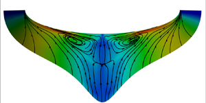
In figure 5(a), we present the temporally averaged azimuthal velocity ${\bar {u}_{\zeta }}$, at ${x = 1250}$ mm, along with the streamlines. The azimuthal mean velocity $\bar {u}_{\zeta }$ is the most prominent within the azimuthal angles $100^{\circ } \lesssim \phi \lesssim 120^{\circ }$. The wall-normal distributions of the mean crossflow velocity, the wall-parallel velocity normal to the near-inviscid stream at the edge of the boundary layer, $\bar {u}_n$ are given in figures 5(b,c) in several meridian planes at $x = 1250$ mm. The crossflow velocity is the strongest at $\eta /\delta \approx 0.2$, with the maximum values less than 0.05$q_{\infty }$ or $u_{\tau }$. Compared to other three-dimensional TBLs (Bentaleb & Leschziner 2013), the mean crossflow velocity in the presently considered flow configuration is much weaker.

Figure 5. Distributions of (a) the azimuthal mean velocity $\bar {u}_{\zeta }$ at $x=1250$ mm overlaid by the streamlines and the wall-normal profiles of the mean crossflow velocity $\bar {u}_n$ normalized by (b) outer and (c) viscous scales.

By inspecting the mean streamlines, we further identify a large circulation zone around $\phi \approx 120^{\circ }$ that brings the high-speed fluids towards the near-wall region adjacent to the attachment lines, and the low-speed fluids upwards near the WSP, reminiscent of the flow field induced by spanwise-opposed wall jet forcing used to reduce the turbulent drag (Yao et al. 2017; Yao, Chen & Hussain 2018). Moreover, there is a sink point in the free-stream of the boundary layer ($\eta \approx 2 \delta$), suggesting that the fluids are converging towards this point as they are brought downstream. These cross-stream motions can be regarded as Prandtl secondary flows of the first kind (Bradshaw 1987), in that the non-zero AoA is responsible for the streamline curvature in the free-stream or at the inviscid limit, leading to the generation of the large-scale circulations that are diffused by viscous and turbulent stresses. Moreover, these streamwise vortices can be observed as well when the boundary layer is laminar, as has been shown in our previous study (Chen et al. 2022), thereby excluding the possibility of them being generated by turbulent stresses, the type of secondary flows generated by the turbulence inhomogeneity and anisotropy (Nezu 2005), namely the Prandtl secondary flows of the second kind. The intensity of the circulation can be quantified as

(3.1)\begin{equation} I_{circ}=\sqrt{\bar{u}_{\eta}^2+\bar{u}_{\zeta}^2}/\bar{u}_{\xi}. \end{equation}

For the presently considered case, the maximum of $I_{circ}$ is approximately $0.06$. Despite their weakness in comparison with the mean flow, these large-scale circulations will lead to dramatic variation of the turbulent statistical properties (Anderson et al. 2015), which will be demonstrated in the next section.

3.2. Skin friction and wall heat transfer

The existence of large-scale circulations significantly modifies the distributions of the skin friction and the wall heat transfer. Figure 6(a) displays the distribution of skin friction

(3.2)\begin{equation} C_f=2\bar{\tau}_{w,\xi}/\rho_{e}q_{e}^2 \end{equation}

on the HyTRV model, overlaid by the wall limiting streamlines, the ‘streamlines’ defined by the wall shear stresses. Apparently, the variation of $C_f$ exhibits differences from those induced by the natural transition processes (Chen et al. 2022; Men et al. 2023). At a given streamwise location, $C_f$ decreases from the attachment lines towards the WSP, accompanied by the thickening of the boundary layer (recall figure 4). The wall limiting streamlines show a tendency to converge, deviating slightly from both the streamwise direction and the meridian planes, suggesting that the near-wall flows incline to bring the fluids from the side attachment lines towards the WSP by, as can be inferred from figure 5, the secondary circulations.

Figure 6. (a) Skin friction $C_f$ (flooded contour) overlaid by the wall limiting streamlines. (b) Streamwise variations of $C_f$. (c) Transformed incompressible skin friction $C_{f,i}$ along the four wall limiting streamlines in (a).

The $C_f$ along the four wall limiting streamlines marked in figure 6(a) (hereinafter referred to as lines 1, 2, 3 and 4) are displayed in figure 6(b). Along line 3 (at least $43^{\circ }$ away from the WSP) and line 4 (at least $55^{\circ }$ away from the WSP), there is an evident overshoot of $C_f$ at $x\approx 800$ mm, which is a typical feature of the transition from laminar to turbulence. Along lines 1 and 2 in or adjacent to the WSP, by contrast, the values of $C_f$ increase gradually downstream, which is in stark contrast to those in canonical TBLs where $C_f$ decreases monotonically once the fully developed turbulent state is attained. Such a difference in the $C_f$ variations can be attributed to two counteracting flow mechanisms. Typically, the streamwise evolution of the boundary layer is accompanied by lower skin friction due to the growth of the boundary layer thickness. However, the secondary circulations near the WSP bring the low-momentum fluids upwards and reduce the mean shear rate close to the wall, leading to the abatement in the effects of reducing $C_f$. Considering that these secondary circulations are the most prominent in the vicinity of the WSP, the effects of their weakening in that region will be the most prominent, leading to the increment of $C_f$. Away from the WSP, the influences of the secondary circulations are recovered to finite levels, thus the variation of $C_f$ follows anew the features of typical transitional and turbulent boundary layers.

Another perspective on skin friction can be obtained by plotting the van Driest II transformed incompressible skin friction $C_{f,i}=F_cC_f$ against $Re_{\theta,i}=Re_{\delta _2}=F_{\theta }\,Re_{\theta }$ (Hopkins & Inouye 1971), with the transformation functions $F_c$ and $F_{\theta }$ defined by

(3.3a,b)\begin{equation} F_c=\frac{r\,\dfrac{\gamma-1}{2}\,Ma_e^2}{(\textrm{arcsin}\,A+\textrm{arcsin}\,B)^2} \quad \textrm{and} \quad F_{\theta}=\mu_{e}/\mu_{w}, \end{equation}

and $A$ and $B$ calculated as

(3.4)\begin{equation} \left.\begin{gathered} A=\frac{2a^2-b}{\sqrt{4a^2+b^2}}\quad \textrm{and} \quad B=\frac{b}{\sqrt{4a^2+b^2}},\\ a= \left(r\,\frac{\gamma-1}{2}\,Ma_{e}^2\,\frac{T_{e}}{T_w}\right)^{1/2} \quad\textrm{and} \quad b=\frac{\bar{T}_{aw}}{T_w}-1, \end{gathered}\right\} \end{equation}

where $\bar {T}_{aw}=(1+r({(\gamma -1)}/{2})\,Ma_{e}^2)T_e$ is the adiabatic wall temperature. The results are plotted in figure 6(c) for $x>950$ mm and compared with the power-law relation $C_{f,i}=0.024\,Re_{\theta,i}^{-0.25}$ for ZPG-TBLs (Smits et al. 1983).

The transformed $C_{f,i}$ along lines 2–4 (downstream of the overshoot position) collapse reasonably well and are slightly higher than the incompressible correlation for ZPG-TBLs, consistent with the observation of Wenzel et al. (2019) in supersonic TBLs subjected to weak and moderate APGs. (We will find in § 3.4 that the TBL presented herein undergoes a mild streamwise APG.) The $C_{f,i}$ along line 1 in the vicinity of the WSP, on the contrary, is significantly lower than the prediction due to the upward motions near the WSP bringing the low-speed fluids upwards to reduce the skin friction.

In figure 7, we present the distribution of the mean wall heat flux

(3.5)\begin{equation} \bar{Q}_w=k\,\partial_{\eta}\bar{T}|_w. \end{equation}

The overall distribution in figure 7(a) and the streamwise variation along the wall limiting streamlines in figure 7(b) bear considerable resemblance to those of the skin friction $C_f$, except for the transitional region. To evaluate their similarities, the Reynolds analogy factor $R_{af}=2C_h/C_f$ is plotted in figure 7(c), where $C_h=\bar {Q}_w/(C_p\rho _{e}q_{e}(T_r-T_w))$ is the Stanton number. Here, $R_{af}$ lies between 1.16 and $Pr^{-2/3}$, and retains almost constant values in the turbulent region, consistent with the results of ZPG-TBLs over flat plates reported by Huang et al. (2022).

Figure 7. (a) Mean wall heat flux $\bar {Q}_w$ (flooded contour) overlaid by the wall limiting streamlines.(b) Streamwise variations of $\bar {Q}_w$. (c) The Reynolds analogy factor $R_{af}$ along the four wall limiting streamlines in (a). Dashed and dash-dotted lines represent, respectively, $Pr^{-2/3}$ and 1.16.

3.3. Three-dimensionality of the mean flow

The cross-stream secondary motions will lead to the mean flow three-dimensionality, namely the mean velocity vector with varying directions along the wall-normal direction, which can be quantified by the deflection of the inviscid stream.

Figure 8(a) displays the angle $\gamma _{v,e}$ between the streamwise and azimuthal mean velocities at the boundary layer edge, with

(3.6)\begin{equation} \gamma_{v}=\textrm{arctan}\left(\frac{\bar{u}_{\zeta}}{\bar{u}_{\xi}}\right) \end{equation}

as a function of the azimuthal angle $\phi$ at three streamwise stations. Here, $\gamma _{v,e}$ shows a consistent variation for several streamwise locations, with its maximum 4.5$^{\circ }$ at $\phi \approx 100^{\circ }$. As it approaches the WSP, $\gamma _{v,e}$ gradually decreases and remains less than $1^\circ$ within the region $\phi \approx 180^{\circ }\pm 40^{\circ }$. The angle between the streamwise and azimuthal wall shear stresses is reported as well, defined as

(3.7)\begin{equation} \gamma_{\tau_w}=\textrm{arctan}\left(\frac{\bar{\tau}_{w,\zeta}}{\bar{\tau}_{w,\xi}}\right), \end{equation}

reflecting the trajectories of the wall limiting streamlines. The trend of variation of $\gamma _{\tau _w}$ is similar to $\gamma _{v,e}$ but with higher magnitudes. The discrepancy in the magnitudes of $\gamma _{\tau _w}$ and $\gamma _{v,e}$ suggests the existence of the crossflow. As demonstrated in figure 8(b), the twist angle of the mean velocity vector inside the boundary layer, i.e. $\gamma _v-\gamma _{v,e}$, is highest close to the wall, and decreases almost monotonically as it approaches the edge of the boundary layer, suggesting that the mean velocity vector is progressively twisted towards the wall.

Figure 8. Distributions of (a) $\gamma _{v,e}$ and $\gamma _{\tau _w}$ in the azimuthal direction at $x=1050$, 1250 and 1450 mm. Colour from light to dark represents increasing $x$. (b) Twist angle $\gamma _v-\gamma _{v,e}$ at $x=1250$ mm in the wall-normal direction.

We further remark on the influences of the transverse curvature variation. The significance of such influences can be characterized by the ratio of the boundary layer thickness to the curvature radius $\delta /r_s$ and the curvature-radius-based Reynolds number $r_s^+=r_s/\delta _{\nu }$. Based on these two parameters, the flow regimes can be classified into three categories: (i) large $r_s^+$ and large $\delta /r_s$, (ii) small $r_s^+$ and large $\delta /r_s$, and (iii) large $r_s^+$ and small $\delta /r_s$ (Piquet & Patel 1999). For the presently considered TBL over the HyTRV, these parameters are $\delta /r_s \lesssim 0.8$ and $r_s^+ \gtrsim 1500$ on the windward side ($x>1000$ mm), falling into the third regime, indicating that the TBL over the windward side is similar to that over a flat plate, so that the three-dimensionality effects are indeed weak.

3.4. Pressure gradient

Despite the insignificance of the curvature on the windward side, the curvature radius of the HyTRV model at each streamwise station is not azimuthal-invariant and inevitably induces the azimuthal pressure gradient. Moreover, a non-zero AoA will also lead to APG. The effects of the mean pressure gradients will be considered in this subsection.

The global distribution of the mean wall pressure $\bar {p}_w$ is shown in figure 9(a), and the azimuthal variations at $x=1050$, 1250 and 1450 mm in figure 9(b). The $\bar {p}_w$ value reaches its peak at $\phi \approx 92^{\circ }$, where there are no turbulent fluctuations, and then drops rapidly with increasing $\phi$ until $\phi \approx 120^{\circ }$, beyond which it remains an almost constant value. Since the HyTRV model is diverging in the streamwise direction, the azimuthal extent in terms of the arc length with nearly constant wall pressure therefore gets larger as it approaches downstream, suggesting the progressively weaker influences of the azimuthal pressure gradient. Nevertheless, the transverse pressure gradient constantly drives lateral flows towards the WSP where the upwelling motions are formed, yielding the formation of large-scale cross-stream circulations.

Figure 9. Distributions of the mean wall pressure $\bar {p}_w$ (a) on the lower wall of the HyTRV, (b) in the azimuthal direction at $x=1050$, 1250 and 1450 mm, and (c) along the streamwise direction in meridian planes ${\phi =140^{\circ }}$ and $180^{\circ }$, with the parameter $\beta _K$ shown in the inset, and dashed lines denoting the boundaries of the blowing/suction slot.

It is also noteworthy that $\bar {p}_w$ near the WSP increases mildly in the streamwise direction, as indicated by the arrow in figure 9(b), implying the existence of streamwise APG. For the purposes of illustration, in figure 9(c) we display the streamwise variation of $\bar {p}_w$ in the WSP and $\phi =140^\circ$. Except for the regions of blowing/suction disturbances introduced on the wall, where the mean pressure drops significantly, $\bar {p}_w$ in general keeps increasing in the streamwise direction, confirming the existence of APG. According to Gibis et al. (2019), the strength of the streamwise APG can be evaluated by the kinematic Rotta–Clauser parameter, defined as

(3.8a,b)\begin{equation} \beta_K= \frac{\delta_{i}^*}{\bar{\tau}_{w,\xi}}\, \frac{\textrm{d}\bar{p}_w}{\textrm{d}\xi},\quad \delta_{i}^*=\int_{0}^{\delta} \left(1-\frac{\bar{u}_{\xi}}{\bar{u}_{\xi,e}} \right)\textrm{d}\eta, \end{equation}

which is intended to characterize the self-similar state of compressible APG-TBLs. The streamwise distribution of $\beta _K$ is shown in the inset of figure 9(c), exhibiting a significant variation in the region $950\ \textrm{mm} \lesssim x \lesssim 1100\ \textrm {mm}$, with its maximum $\beta _{K,max}\approx 0.6$ at $x\approx 1000$ mm. As it goes further downstream of $x\approx 1100$ mm, $\beta _K$ remains less than 0.25 and exhibits azimuthal independence, as suggested by the almost collapsed mean distribution in meridian planes $\phi =140^\circ$ and $\phi =180^\circ$. The low-levelled $\beta _K$ indicates the weakness of the streamwise APG and its possibly trivial effects compared with the mild APG-TBLs reported by Kitsios et al. (2017) over flat plates, and moreover, the significance of the dynamic roles of the secondary circulations, which is perhaps the only reason that leads to the differences of statistics in the azimuthal direction.

It is of interest here to examine the effects of the weak APG on the wall pressure fluctuations. Huang et al. (2022) found that the intensities of wall pressure fluctuation $p_{w,rms}$ normalized by the mixing scaling $\rho _wu_{\tau }q_{\infty }$ yield the best collapse for compressible TBLs with different $Ma_{\infty }$ and wall temperature ratios compared to the inner scaling $\bar {\tau }_w$ and the mean wall pressure $\bar {p}_w$. Plots of $p_{w,rms}/\rho _wu_{\tau }q_{\infty }$ along the above-mentioned four limiting streamlines are provided in figure 10 and compared with those in high-speed flat-plate ZPG-TBLs with $5\leqslant Ma_{\infty }\leqslant 14$ and $0.18\leqslant T_w/T_r \leqslant 0.91$ (Huang et al. 2022). Along lines 2–4, $p_{w,rms}/\rho _wu_{\tau }q_{\infty }$ values show slight scatter and agree reasonably well with values obtained by Huang et al. (2022), and they are much lower than those along line 1. Such a discrepancy between line 1 and other lines is due not to the difference of the pressure gradient as indicated by figure 9(c), but to the large-scale secondary circulations that significantly reduce the friction velocity in the WSP. The effects of APG on the fluctuating wall pressure are therefore difficult to conclude from the present case with $\beta _K\lesssim 0.25$.

Figure 10. Intensities of wall pressure fluctuations in the mixing scaling along the four limiting streamlines (lines 1–4) represented by symbols with increasingly lighter colours.

4. Local turbulence statistics

This section is devoted to comparing flow statistics at certain streamwise and azimuthal locations in the present TBL over the HyTRV with canonical ones over flat plates with or without APG to evaluate their similarities and the extent of the latter replicating the former.

4.1. Mean velocity profiles

The mean velocity profiles and the scaling laws will be considered in this subsection. Figure 11 provides the wall-normal distributions of the mean velocity at five streamwise stations evenly distributed from $x=1050$ to 1450 mm in meridian planes $\phi =140^{\circ }$ and $180^{\circ }$ integrated by the van Driest transformation (van Driest 1951)

(4.1)\begin{equation} \bar{u}_{\xi,VD}^+=\int_{0}^{\bar{u}_{\xi}^+}\sqrt{\frac{\bar{\rho}}{\bar{\rho}_w}}\,\textrm{d}\bar{u}_{\xi}^+, \end{equation}

the total-stress-based transformation (Griffin et al. 2021)

(4.2a,b)\begin{equation} \bar{u}_{\xi,TS}^+=\int_{0}^{\bar{u}^+_{\xi}}\frac{S_{eq}^+}{1+S_{eq}^+-S_{TL}^+}\,\textrm{d}\eta_{TL}^+, \quad \eta^+_{TL}=\frac{\eta(\bar{\rho}\bar{\tau}_{w,\xi})^{1/2}}{\bar{\mu}}, \end{equation}

with the equivalent strain rates defined as

(4.3a,b)\begin{equation} S_{eq}^+=(\bar{\mu}_w/\bar{\mu})(\partial \bar{u}_{\xi}^+{/}\partial \eta^+_{TL}),\quad S_{TL}^+=(\bar{\mu}/\bar{\mu}_w)(\partial \bar{u}_{\xi}^+{/}\partial \eta^+), \end{equation}

and the transformation incorporating intrinsic compressibility effects

(4.4)\begin{equation} \bar{u}_{\xi,H}^+=\int_{0}^{\bar{u}_{\xi}^+} \left(\frac{1+\eta_{TL}D^c\kappa }{1+ \eta_{TL}D^i\kappa}\right)\left(1-\frac{\eta}{\delta_{\mu,TL}}\, \frac{\textrm{d}\delta_{\mu,TL}}{\textrm{d}\eta}\right)\sqrt{\frac{\bar{\rho}}{\rho_w}}\, \textrm{d}\bar{u}_{\xi}^+, \end{equation}

proposed very recently by Hasan et al. (2023), with

(4.5a,b)$$\begin{gather} \delta_{\mu,TL}=\frac{\bar{\mu}}{\bar{\rho}}\,\sqrt{\frac{\bar{\rho}}{\bar{\tau}_w}},\quad D^c=\left[1-\exp\left(\frac{-\eta_{TL}}{A^++f(M_{\tau})}\right)\right]^2, \end{gather}$$

(4.5c)$$\begin{gather}D^i=[1-\exp(-\eta^+{/}A^+)]^2, \end{gather}$$

$f(M_{\tau })=19.3M_{\tau }$ (where $M_{\tau }=u_{\tau }/\sqrt {\gamma R T_w}$ is the friction Mach number), $A^+=17$, and the Kármán constant $\kappa =0.41$.

Figure 11. Wall-normal distributions of the mean velocity integrated by (a,b) the van Driest transformation, (c,d) the total-stress-based transformation (Griffin et al. 2021), and (e,f) the transformation incorporating intrinsic compressibility effects (Hasan et al. 2023), in meridian planes (a,c,e) $\phi =140^{\circ }$ and (b,d,f) $\phi =180^{\circ }$. Insets are the enlarged views in the viscous layer.

Bai, Griffin & Fu (2022) found that van Driest (van Driest 1951), Zhang (Zhang et al. 2012), Trettel–Larsson (Trettel & Larsson 2016), data-driven (Volpiani et al. 2020) and total-stress-based (Griffin et al. 2021) transformations satisfactorily collapse the mean velocity profiles in adiabatic TBLs with weak APGs (with $\beta _K$ up to 0.69 using data from Wenzel et al. 2019) to the incompressible reference. This conclusion very likely can be extended to TBLs with moderately cooled walls and weak APG since the transformed mean velocities integrated by these formulas displayed in figure 11 obey the linear law within the viscous sublayer and the logarithmic law in the vicinity of $\eta ^+ \approx 100$ and $\eta ^+_{TL} \approx 100$, with the slope and the intercept of the latter being $1/\kappa$ and $C=5.2$, the same as those in incompressible ZPG-TBLs. To be more specific, in the viscous layer, as shown by the insets, the total-stress-based transformation and the transformation incorporating intrinsic compressibility effects give almost indistinguishable results and perform better than the van Driest transformation, which is known to yield a smaller slope for cooled-wall TBLs (Zhang et al. 2018). The average slope of the van Driest transformed mean velocity below $\eta ^+=5$ is about 0.897, which is 10 % lower than those obtained by the other two transformations. In the logarithmic layer, the transformation incorporating intrinsic compressibility effects yields the best collapse in meridian plane $\phi =140^{\circ }$ compared to the other two transformations, but its performance deteriorates in the WSP, where the scatter is more significant than the other two transformations, which have comparable performance and do not show such an azimuthal dependence. In the wake region, the mean velocities are progressively enhanced as it approaches the WSP, reminiscent of TBLs subject to the streamwise APG, as suggested by the results reported by Sanmiguel Vila et al. (2017) with $\beta =2$ shown in figure 11.

To further investigate the universalities of the mean velocity in the outer layer, in figure 12 we display the mean velocity deficit under outer scalings in meridian plane $\phi =140^{\circ }$ (figures 12a,c,e) and the WSP (figures 12b,d,f) at five streamwise stations distributed evenly between $x=1050$ and 1450 mm. When normalized by the free-stream values of the van Driest transformed mean velocity and plotted against the outer scale $\eta /\delta$, as shown in figures 12(a,b), the mean velocity deficits are scattered in each meridian plane at varying streamwise locations. The total-stress-based transformation works better in collapsing the mean velocity deficits (figures 12c,d), but when compared with the results from an incompressible canonical TBL reported by Sillero, Jiménez & Moser (2013) and incompressible flat-plate APG-TBLs with $\beta =0.7{-}2.2$ by Sanmiguel Vila et al. (2020b), deviations are still prominent, requiring further efforts to collapse them onto a single curve.

Figure 12. Mean velocity deficit profiles in meridian planes (a,c,e) $\phi =140^{\circ }$ and (b,d,f) $\phi =180^{\circ }$ expressed as (a,b) $1-\bar {u}_{\xi,VD}/\bar {u}_{\xi,VD,e}$, (c,d) $1-\bar {u}_{\xi,TS}/\bar {u}_{\xi,TS,e}$, and (e,f) $(\tilde {u}_{\xi,e}-\tilde {u}_{\xi })/u_{ZS}$, with $u_{ZS}$ the Zagarola–Smits velocity scale.

There are multiple factors that could lead to such inconsistency, one of which is the mean APG, which can be incorporated by the Zagarola–Smits velocity scale defined as ${u_{ZS}=\tilde {u}_{\xi,e}\delta _i^*/\delta}$, with $\delta ^*_i$ the incompressible displacement thickness. As has been demonstrated by Gibis et al. (2019), for a given APG strength $\beta _K$, the Zagarola–Smits velocity scale is capable of collapsing the mean velocity deficit profiles at various streamwise locations in supersonic APG-TBLs so that the outer-layer self-similarity can be satisfied. The Zagarola–Smits scaling is also examined in the present hypersonic TBL, as displayed in figures 12(e,f). As a comparison, we also display the results from an incompressible canonical TBL (Sillero et al. 2013), a supersonic flat-plate APG-TBL at $Ma_{\infty }=2$ and $\beta _K=0.55$ (Gibis et al. 2019), and incompressible flat-plate APG-TBLs (Sanmiguel Vila et al. 2020b). These results are consistent with statistics in the present study in the meridian plane $\phi =140^{\circ }$ with comparatively weak APG, despite the different Reynolds number $Re_\tau$, strengths of APG $\beta$ and the free-stream Mach numbers $Ma_\infty$. As it approaches the WSP, however, the mean velocity deficit profiles within $0.1\lesssim \eta /\delta \lesssim 0.8$ gradually level off so that a stronger embedded shear layer appears in the outer layer, manifesting remarkable differences from the reference data even though the streamwise pressure gradient barely changes from $\phi =140^{\circ }$ to $180^{\circ }$ (figure 9c). From another perspective, the mean velocities do not obey the outer-layer similarity in the azimuthal direction at a given streamwise location under the Zagarola–Smits scaling, suggesting that the TBL over the HyTRV cannot be simplified like those over flat plates with APG. Recalling the discussions in §3 regarding the global flow organization, the differences in the mean velocity at various azimuthal angles should be associated with the secondary circulations. Away from the WSP, where APG plays the dominant role, the mean velocity deficits follow those of the APG-TBLs over flat plates, whereas near the WSP, the effects of the secondary circulations that bring the low-speed fluids upwards are the most intense, leading to the higher intensity of embedded shear layer in the outer region.

To summarize, in the near-wall region, the local mean velocity distributions conform with those of canonical ZPG-TBLs in that the linear and logarithmic laws can be satisfied by performing integral transformations. In the outer layer, the mean velocity deficits are well collapsed with those of APG-TBLs under the Zagarola–Smits velocity scale in the region away from the WSP dominated by merely the APG, whereas evident deviations can be observed near the WSP where the upwelling currents induced by the large-scale circulations are prominent.

4.2. Reynolds stresses

In this subsection, we consider the local distributions of the Reynolds stress components and their variations in the streamwise and azimuthal directions. The Reynolds stresses normalized by viscous scales, defined as

(4.6)\begin{equation} R^+_{ij}=\frac{\overline{\rho u''_i u''_j}}{\bar{\tau}_{w,\xi}}, \end{equation}

are shown in figure 13 along with the statistics of incompressible TBLs over flat walls with and without APG reported in previous studies (Sillero et al. 2013; Sanmiguel Vila et al. 2017). The abscissae are normalized by the semi-local scalings $\eta ^+_{TL}$, which is known to show better universality of $R_{ij}^+$ in the near-wall region at different Mach numbers and wall temperatures (Zhang et al. 2018, 2022; Huang et al. 2022).

Figure 13. Wall-normal distributions of the Reynolds stresses against the semi-local coordinate $\eta ^+_{TL}$, for (a,b) $R^+_{11}$, (c,d) $R^+_{22}$, (e,f) $R^+_{33}$, (g,h) $-R^+_{12}$, with (a,c,e,g) $x=1250$ mm and various azimuthal angles ($\phi =130^{\circ }$ to the WSP), and (b,d,f,h) in the WSP from $x=1050$ to 1450 mm.

In figure 13(a), we present the streamwise normal component $R^+_{11}$ at $x=1250$ mm at various azimuthal angles. Along the azimuthal direction at $x=1250$ mm, where the friction Reynolds numbers $Re_\tau$ are approximately 1150–1200, $R^+_{11}$ follows the same trend of variation in the wall-normal direction as those of canonical TBLs over flat walls, in that the profiles near the wall are well collapsed and the peaks are attained at $\eta ^+_{TL} \approx 15$ in the buffer layer. As it approaches the WSP from the attachment lines, the peaks of $R^+_{11}$ first increase and then decrease to a level lower than that of incompressible TBLs with ZPG. In the outer layer, a secondary peak gradually emerges with an increasingly larger magnitude as it approaches the WSP. The manifestation of the outer peak is, in a way, similar to TBLs with APG, but it requires a much stronger APG to exhibit a high value in the latter ($\beta = 1.3$ and 2.4) (Sanmiguel Vila et al. 2017). Considering that the values of $\beta _K$ in the present study remain low (approximately 0.25) and that their variations in the azimuthal direction are insignificant, it is irrational to ascribe the enhancement of the outer peak to APG. We can infer from the increasing production of the turbulent kinetic energy $P_K$ – cast as the multiplication of the Reynolds shear stress $R_{12}$ and the mean shear $\partial \bar u_{\xi }/\partial \eta$, both of which are increased in the outer layer – that the rate of kinetic energy transferred from the mean to fluctuating velocity is higher, leading to the higher turbulent intensities. In other words, the intensified Reynolds stresses should be attributed to the large-scale cross-stream circulations. This will be demonstrated in detail in the next subsection.

The physical counterparts leading to the increment of the outer peaks are, in all probability, the large-scale low-momentum structures that are similar to the very-large-scale motions (VLSMs) in high-Reynolds-number wall-bounded turbulence (Lee & Sung 2011, 2013; Pirozzoli & Bernardini 2013). These structures, if no other effects are taken into account, usually penetrate into the near-wall region, leaving large-scale ‘footprints’ that enhance the level of the inner peaks. This partially explains the variation of the inner peaks of $R^+_{11}$ – the synchronized increment of the outer and inner turbulent intensities from $\phi =130^\circ$ to $\phi =160^\circ$. As it further approaches the WSP, where the flow is dominated by the upwelling instead of circulations, the inner peaks are decreased, which is caused by either the disruption of the near-wall motions or the detachment of the VLSMs from the wall.

To validate such postulations, in figure 14 we present the streamwise velocity fluctuations $u'^+_\xi$ in three off-wall $(\xi,\zeta )$ planes, in the near-wall region at $\eta ^+ = 15$, slightly above the logarithmic layer at $\eta =0.3 \delta$, and in the outer layer at $\eta =0.6 \delta$. The $u'^+_\xi$ at $\eta ^+ = 15$ is still organized as streamwise elongated streaky structures that are commonly observed in canonical TBLs. Such a flow organization manifests no evident variations in the azimuthal direction, suggesting that the near-wall motions are not, at least visually, disrupted by the upwelling currents in the vicinity of the WSP. The flow structures at $\eta =0.3 \delta$ are organized as large-scale high- and low-momentum regions with the spanwise width of the boundary layer thickness, reminiscent of VLSMs in high-Reynolds-number wall-bounded turbulence (Smits, McKeon & Marusic 2011). These VLSMs appear to be capable of penetrating through and reaching down to the near-wall region, leaving large-scale imprints at $\eta ^+ = 15$. Notably, there appears to be no sign of azimuthal dependence of the intensities of the VLSMs. Only at $\eta = 0.6\delta$ can it be observed that the velocity fluctuations are enhanced near the WSP. However, these intensified flow structures are shorter in the streamwise direction compared with those away from the WSP ($\phi < 160^\circ$ or $\phi > 200^\circ$), and, more importantly, differ greatly in morphology from the flow structures at $\eta =0.3 \delta$, leaving no imprints on either $\eta =0.3 \delta$ or $\eta ^+ = 15$. We can conclude from these phenomena that the intensified peaks in the outer layer located at $\eta \approx 0.6\delta$ are detached from the wall, having different morphology and dynamics than the VLSMs that are commonly found in high-Reynolds-number TBLs. Considering the features of the mean velocity in figure 12, we conjecture that these intensified flow structures could be caused by the Kelvin–Helmholtz instability due to the existence of the inflection point (Schatzman & Thomas 2017). This will be discussed in detail in the next subsection.

Figure 14. Instantaneous velocity fluctuations $u'^+_\xi$ in the $(\xi,\zeta )$ planes at (a) $\eta ^+ = 15$, (b) $\eta =0.3 \delta$,(c) $\eta =0.6 \delta$.

Along the streamwise direction in the WSP (figure 13b), the outer peaks manifest monotonic abatement, suggesting the weakening of the VLSMs lying in the upwelling low-momentum region. The inner peaks do not exhibit a simple trend of variation. This is probably due to two counteracting effects: one is the increment of the friction Reynolds number $Re_\tau$ in the streamwise direction (figure 3), and the other is the weakening of the VLSMs, similar to the observations in the recovery downstream of the shock/TBL interactions (Yu et al. 2023).

Regarding the rest of the Reynolds stress components $R^+_{22}$, $R^+_{33}$ and $-R^+_{12}$, the outer peaks are more prominent than the inner ones (if any). They share a common feature that the peaks are enhanced as it approaches the WSP at a certain streamwise station, but weakened downstream in the WSP. Compared with the incompressible APG-TBL with a comparable $Re_{\tau }$ (Sillero et al. 2013), these components are stronger even though the APG is much weaker, indicating anew that the enhancement of the outer peaks should be attributed to the large-scale cross-stream circulations. In the near-wall region, the variations of $R^+_{22}$ and $R^+_{33}$ along the azimuthal direction are consistent with the trend in the outer region, suggesting the comparatively large impacts of VLSMs on the near-wall turbulence. It is noteworthy, however, that the $R^+_{22}$ component, commonly regarded as the wall-detached flow quantity that should be independent of the superposition effects of the VLSMs in the outer region, is augmented as well, not least in the WSP, further proving that the near-wall turbulence is probably disrupted by the upwelling currents. As for the Reynolds shear stress $-R^+_{12}$, its variation trend is consistent with that of $R^+_{11}$ and should share similar properties.

The distributions of the Reynolds stresses in the WSP, as displayed in figure 15 for $R_{11}$ and $R_{22}$, can be collapsed when normalized by the Zagarola–Smits scaling and plotted by outer coordinates; the peaks thereof lie at $\eta \approx 0.6\delta$, which are much higher than the typical VLSMs in ZPG-TBLs located at $\eta = (0.2{-}0.3) \delta$ (Hutchins & Marusic 2007; Marusic, Mathis & Hutchins 2010). However, the Reynolds stresses normalized this way agree with those in APG-TBLs over flat plates (Gungor et al. 2020; Sanmiguel Vila et al. 2020b) only beyond $\eta /\delta \approx 0.7$. The locations and magnitudes of the outer peaks in APG-TBLs under the Zagarola–Smits scaling depend on the shape factor, APG strength, and probably other factors.

Figure 15. Wall-normal distributions of (a) $R_{11}/u_{ZS}^2$ and (b) $R_{22}/u_{ZS}^2$ in the WSP from $x=1050$ to 1450 mm.

The recent study of Wei & Knopp (2023) proposed a novel outer scaling of the streamwise mean momentum equation for TBLs with APG, hereafter referred to as the WK scaling. In the WK scaling, the outer peak location of $R_{12}$ (denoted by the subscript $OP$) is employed to determine proper scalings as

(4.7)$$\begin{gather} \eta^*=(\eta-\eta_{OP})/(\delta-\eta_{OP}), \end{gather}$$

(4.8)$$\begin{gather}\bar{u}_{\xi}^*=(\bar{u}_{\xi,e}-\bar{u}_{\xi})/(\bar{u}_{\xi,e}-\bar{u}_{\xi,OP}) \end{gather}$$

and

(4.9)\begin{equation} R_{12}^*=R_{12}/R_{12,OP}. \end{equation}

As shown in figure 16(a), the mean velocity deficits $\bar {u}_{\xi }^*$ in the WSP at different streamwise stations and at $x=1050$ mm and $\phi =160^{\circ }$ are well collapsed and consistent with the approximate formula expressed as the error function

(4.10)\begin{equation} F_{WK} = 1 - {\rm erf}(1.3 \eta^* + 0.21(1.3 \eta^*)^4). \end{equation}

Similar conclusions can be drawn for the Reynolds shear stress $R_{12}^*$ (figure 16b) that appears in the streamwise mean momentum equation, with the approximate formula cast as

(4.11)\begin{equation} G_{WK} = 1 - \exp (-(1.3 \eta^*)^2 - 0.385 (1.3 \eta^*)^4). \end{equation}

Although not mentioned in the study of Wei & Knopp (2023), we found that the elucidations can be applied to other Reynolds stress components $R_{11}^*$, $R_{22}^*$ and $R_{33}^*$ as well, with the exact form of the approximate formula (4.11) (see figure 16c for $R_{11}^*$). The implication is that the mean velocity and all the Reynolds stress components are self-similar if properly scaled.

Figure 16. Wall-normal distributions of (a) velocity deficit $\bar {u}^*_{\xi }$, (b) Reynolds shear stress $R_{12}^*$ and(c) streamwise Reynolds normal stress $R_{11}^*$.

4.3. Outer layer turbulence amplification

As illustrated in the previous subsection, the highly intensified turbulent kinetic energy in the outer region can be explained in terms of its production. However, there is a setback in such an inference in that the generation of the Reynolds shear stress remains unknown, requiring further exploration from the perspective of flow dynamics.

Figure 17 displays the rescaled mean velocity gradient in the WSP. Due to the presence of large-scale secondary circulations flanking the WSP (figure 5), there manifests an inflection point in the outer layer at $\eta /\delta \approx 0.66$, in spite of the smallness of the APG that implies that no flow separation should be expected (Kitsios et al. 2017; Gungor, Maciel & Gungor 2022). The appearance of these inflection points and their locations away from the wall suggest that the inflectional Kelvin–Helmholtz instability is probably responsible for the amplified outer-layer turbulence.

Figure 17. Mean velocity gradient $\bar \rho \,\textrm {d} \tilde u_{\xi }/\textrm {d}\eta$ in the WSP at different streamwise stations.

It has been proven by Schatzman & Thomas (2017) that the Kelvin–Helmholtz instability leads to large-scale spanwise-oriented rollers centred at the inflection point, transferring the comparatively low-speed fluid upwards and high-speed fluid downwards, and thereby resulting in the significant contribution to the Reynolds shear stress. To verify whether this is also the case for the presently considered flow, we obtain the wall-normal distributions of the Reynolds shear stress carried by these upward and downward turbulent transports, namely the ejection (Q2) and sweeping (Q4) events, respectively, conditioned to

(4.12)\begin{equation} |u_{\xi}'(\eta)\,u_{\eta}'(\eta)|>\alpha_q\,u_{\xi,rms}(\eta)\,u_{\eta,rms}(\eta), \end{equation}

with $\alpha _q$ the threshold set as $3.0$. The results in the meridian planes $\phi = 160^{\circ }$ and $\phi = 180^{\circ }$ (WSP) at $x=1050$ mm are shown in figure 18, along with the mean velocity and the normalized streamwise velocity fluctuation intensity. In $\phi = 160^{\circ }$ without mean velocity inflection points, Q2 events play a dominant role compared with the Q4 events in contributing to the Reynolds shear stress across the boundary layer. In $\phi = 180^{\circ }$, however, the Reynolds shear stress carried by the Q4 events exceeds that of Q2 events below the inflection point, while the opposite is true above that point, with the peaks thereof located below and above the inflection points, respectively. This indicates that the large-scale spanwise-oriented rollers induced by the Kelvin–Helmholtz instability do exist in the WSP and should be the primary cause of turbulence amplification in the outer layer, consistent with the elucidations given by Schatzman & Thomas (2017) in a highly decelerated unsteady TBL.

Figure 18. Wall-normal distributions of the tangential Reynolds stresses $-\overline {u_{\xi }'u_{\eta }'}^+$ carried by ejection (Q2, $u_{\xi }'<0, u_{\eta }'>0$) and sweeping (Q4, $u_{\xi }'>0, u_{\eta }'<0$) events, the mean velocity $\bar {u}_{\xi }/q_{\infty }$ and the normalized streamwise velocity fluctuation intensity $\overline {u_{\xi }'^{2}}/\overline {(u_{\xi }'^{2})}_{max}$ in meridian planes (a) $\phi =160^{\circ }$ and (b) $\phi =180^{\circ }$ at $x=1050$ mm.

Recalling figure 13 that presents the distribution of the Reynolds stress components, the amplified outer peaks can be observed only close to the WSP and are weakened downstream. Since the inflection points of the mean velocity can be observed merely along the meridians around the WSP within a small azimuthal angle, we can infer that the outer peaks at $\phi =160^\circ$ and $140^\circ$ should be ascribed to the diffusion and convection of the turbulent kinetic energy from the WSP instead of the inherent Kelvin–Helmholtz instability.

4.4. Contribution of the embedded shear layer to the mean skin friction

As a wall quantity, the mean skin friction presented in figure 6 is closely related to the turbulent statistics inside boundary layers. Therefore, understanding the generation of skin friction is crucial for the drag reduction of high-speed vehicles. In canonical wall-bounded turbulence, previous studies (Renard & Deck 2016; Li et al. 2019; Tong et al. 2022) found that the turbulence kinetic energy production $P_K$ contributes the most to the skin friction using the Renard–Deck formula (Renard & Deck 2016). The outer-layer peaks of the tangential Reynolds stress (figure 13) and the mean velocity gradient (figure 17) indicate the presence of an outer-layer peak of $P_K$ near the WSP, and consequently a significant contribution of the embedded shear layer to the skin friction, which will be quantified in this subsection. Before going further with this issue, we first perform a decomposition of the mean skin friction, following Renard & Deck (2016) and Li et al. (2019):

(4.13)\begin{equation} C_f=C_{f,V}+C_{f,T}+C_{f,G}. \end{equation}

These three right-hand-side terms are expressed as

(4.14a)$$\begin{gather} C_{f,V}=\frac{2}{\rho_{e}\tilde{u}_{\xi,e}^3}\int_{0}^{\delta}\bar{\tau}_{\nu,\xi\eta}\,\frac{\partial \tilde{u}_{\xi}}{\partial \eta}\,\textrm{d}\eta, \end{gather}$$

(4.14b)$$\begin{gather}C_{f,T}=\frac{2}{\rho_{e}\tilde{u}_{\xi,e}^3}\int_{0}^{\delta}\bar{\tau}_{t,\xi\eta}\,\frac{\partial \tilde{u}_{\xi}}{\partial \eta}\,\textrm{d}\eta, \end{gather}$$

(4.14c) \begin{gather} C_{f,G}=\frac{2}{\rho_{e}\tilde{u}_{\xi,e}^3}\int_{0}^{\delta}(\tilde{u}_{\xi}-\tilde{u}_{\xi,e}) \bar{\rho}\left(\tilde{u}_{\xi}\, \frac{\partial \tilde{u}_{\xi}}{\partial \xi}+\tilde{u}_{\eta}\,\frac{\partial \tilde{u}_{\xi}}{\partial \eta}\right)\textrm{d}\eta\nonumber\\ \qquad -\,\frac{2}{\rho_e\tilde{u}_{\xi,e}^3}\int_{0}^{\delta}(\tilde{u}_{\xi}-\tilde{u}_{\xi,e})\, \frac{\partial}{\partial \xi}(\bar{\tau}_{t,\xi\xi}+\bar{\tau}_{\nu,\xi\xi})\,\textrm{d}\eta\nonumber\\ +\,\frac{2}{\rho_e\tilde{u}_{\xi,e}^3}\int_{0}^{\delta}(\tilde{u}_{\xi}-\tilde{u}_{\xi,e})\, \frac{\partial \bar{p}}{\partial \xi}\,\textrm{d}\eta, \end{gather}

denoting the contributions of the viscous dissipation, turbulent kinetic energy production and streamwise heterogeneity, respectively, where the viscous shear stress is $\bar {\tau }_{\nu,ij}=\bar {\mu }(\partial \bar {u}_i/\partial x_j+\partial \bar {u}_j/\partial x_i)$ and the Reynolds shear stress is $\bar {\tau }_{t,ij}=\bar {\rho }(-\widetilde {u_i''u_j''})$. Despite the formulas above being derived for two-dimensional TBLs, they can be readily applied here as well, because the relative error of the summation of the right-hand-side terms in (4.13) obtained by turbulent statistics compared with $C_f$ is less than $0.1\,\%$, suggesting that the three-dimensional effects are indeed trivial, at least in contributing to the skin friction.

Figure 19 displays the streamwise distribution of $C_f$ in the meridian planes $\phi =140^{\circ }$ and $180^{\circ }$. In the former away from the WSP, the contributions of each term on the right-hand-side of (4.13) to the skin friction $C_f$ are generally similar to those in canonical TBLs (Li et al. 2019; Tong et al. 2022), in that the viscous dissipation $C_{f,V}$, turbulent production $C_{f,T}$ and streamwise heterogeneity $C_{f,G}$ terms constitute approximately 35 %, 50 % and 15 % of $C_f$, respectively. In the WSP, the contribution of the viscous dissipation $C_{f,V}$ remains low, while the other two components are highly different from those of canonical TBLs. The turbulent production term $C_{f,T}$ reaches a level even higher than $C_f$ itself, which should be caused by the high-rising peaks of the Reynolds shear stress $-R_{12}$ in the outer layer that are induced by the Kelvin–Helmholtz instability. The $C_{f,G}$ term is no longer positive as in $\phi =140^{\circ }$, but it shows a tendency of recovering towards positive values along the streamwise direction.

Figure 19. The streamwise variations of the decomposed skin friction components in meridian planes(a) $\phi =140^{\circ }$ and (b) $\phi =180^{\circ }$ (WSP).

We have seen in the subsections above that moving towards the WSP is similar to increasing APG strength in flat-plate TBLs; consequently, the variation of the importance of the three decomposed terms from plane $\phi =140^{\circ }$ (figure 19a) to the WSP (figure 19b) resembles that in TBLs with increasing APG strength (Fan et al. 2020), i.e. $C_{f,T}/C_f$ increases dramatically to be the dominant contributor, $C_{f,V}/C_f$ becomes negligible, and $C_{f,G}/C_f$ becomes negative.

The study of Renard & Deck (2016) has pointed out that one of the necessary conditions of the positiveness of $C_{f,G}$ is that the total shear stress should decrease monotonically along the wall-normal direction. This is indeed the case in TBLs with ZPGs and in $\phi =140^\circ$ in the present study, but obviously not in the WSP, as indicated by the high extending peaks of $-R_{12}$, one significant component constituting the total shear stress, in the outer layer. In the aspect of physical significance, the $C_{f,G}$ term represents the mean kinetic energy transfer from the TBLs to the free-stream in the absolute frame, the one travelling with the free-stream velocity. In the wall reference frame, it is related to the growth of the boundary layer that absorbs the energy from the free-stream, or equivalently, the viscous dissipation. In the study of Yu et al. (2023) that discussed the negative $C_{f,G}$ during the turbulence recovery downstream of the shock/TBL interactions, incompatible growth rates were found between the nominal and kinetic energy thicknesses, with the former much higher than the latter, suggesting that the kinetic energy dissipation per unit length is lowered. This is also the case for the presently considered TBL in the WSP and its neighbourhood (omitted for brevity), in that the ratio between the kinetic energy thickness and the nominal thickness is lower as it approaches downstream. Therefore, we conclude that the negative $C_{f,G}$ should be attributed to the reduced energy absorption compared with the ZPG-TBLs.

After having a general impression of the relation between turbulent statistics and the mean skin friction, we further quantify the contribution of the embedded shear layer induced by the Kelvin–Helmholtz instability to the mean skin friction in the WSP. For that purpose, we decompose the mean velocity and the Reynolds shear stress into two portions: the canonical portion ZPG-TBL (denoted by the subscript $c$), and the other corresponding to the embedded shear layer (denoted by $s$).

Following Yu et al. (2023), the mean velocity is split as

(4.15)\begin{equation} \tilde{u}_{\xi}=\tilde{u}_{\xi,s}+\tilde{u}_{\xi,c}, \end{equation}

in which the van Driest transformation of the canonical mean velocity $\tilde {u}_{\xi,c}$ is constructed as

(4.16)\begin{equation} \tilde{u}_{\xi,c,VD}(\eta^+)=\int_{0}^{\eta^+}\left[-\frac{1}{2\,\lambda(s)^2} +\frac{1}{2\,\lambda(s)^2}\left(1+4\,\lambda(s)^2\left(1-\frac{s}{Re_{\tau}}\right)\right)^{1/2}\right]\textrm{d}s, \end{equation}

the universal mean velocity profile proposed by Subrahmanyam, Cantwell & Alonso (2022), with $\lambda (s)$ the mixing length model introduced by Cantwell (2019). Similarly, the mean total stress can be decomposed as

(4.17)\begin{align} \bar{\tau}&=\bar{\tau}_{\nu}+\bar{\tau}_{t}\nonumber\\ &=\bar{\tau}_{\nu,c}+\bar{\tau}_{t,c}+\bar{\tau}_{\nu,s}+\bar{\tau}_{t,s}\nonumber\\ &=\bar{\tau}_{c}+\bar{\tau}_{\nu,s}+\bar{\tau}_{t,s}, \end{align}

where $\bar {\tau }_{\nu }$ and $\bar {\tau }_{t}$ denote the viscous and Reynolds shear stresses, respectively. The Reynolds shear stress induced by the embedded shear layer is therefore cast as

(4.18)\begin{equation} \bar{\tau}_{t,s}=\bar{\tau}-\bar{\tau}_{c}-\bar{\tau}_{\nu,s}, \end{equation}

where the viscous shear stress induced by the embedded shear layer $\bar {\tau }_{\nu,s}$ is determined by the mean velocity of the embedded shear layer $\bar {u}_s$. The total shear stress contributed by the canonical ZPG-TBL $\bar {\tau }_{c}$ is obtained via the formula proposed by Kumar & Mahesh (2021).

Substituting $\tilde {u}_{\xi }=\tilde {u}_{\xi,s}+\tilde {u}_{\xi,c}$ and $\bar {\tau }_{t}=\bar {\tau }_{t,s}+\bar {\tau }_{t,c}$ into $C_{f,V}$ and $C_{f,T}$, we have

(4.19a)$$\begin{gather} C_{f,V,c}=\frac{2}{\rho_{e}\tilde{u}_{\xi,e}^3}\int_{0}^{\delta}\bar{\tau}_{\nu,\xi\eta,c}\,\frac{\partial \tilde{u}_{\xi,c}}{\partial \eta}\,\textrm{d}\eta, \quad C_{f,V,s}=C_{f,V}-C_{f,V,c}, \end{gather}$$

(4.19b)$$\begin{gather}C_{f,T,c}=\frac{2}{\rho_{e}\tilde{u}_{\xi,e}^3}\int_{0}^{\delta}\bar{\tau}_{\nu,\xi\eta,t}\,\frac{\partial \tilde{u}_{\xi,c}}{\partial \eta}\,\textrm{d}\eta, \quad C_{f,T,s}=C_{f,T}-C_{f,T,c}. \end{gather}$$

The streamwise variations of $C_{f,T,c}$ and $C_{f,T,s}$ are presented in figure 20(a). It is found that $C_{f,T}$ stems primarily from the embedded shear layer, whose contribution declines as it approaches downstream, with the contribution of $C_{f,T,s}$ to $C_{f,T}$ ($C_{f,T,s}/C_{f,T}$) decreases from over 0.8 to about 0.55 in the presented streamwise extent ($C_{f,T,s}/C_{f}$, the contribution of $C_{f,T,s}$ to $C_{f}$, decreases from approximately 1.25 to 0.45). The contribution of the embedded shear layer to the mean skin friction via viscous dissipation $C_{f,V,s}$, on the other hand, is almost negligible compared with the canonical portion $C_{f,V,c}$, as shown in figure 20(b), because the viscous dissipation is dominantly contributed by the canonical portion in the near-wall region.

Figure 20. The skin friction contributed by the canonical portion and the outer embedded shear layer to(a) $C_{f,T}$ and (b) $C_{f,V}$ in the WSP.

The contribution of enhanced outer-layer large-scale structures to the mean skin friction is also considerable in other scenarios. For example, Yu et al. (2023) found that $C_{f,T,s}$ is the dominant contributor of $C_{f,T}$ near the shock/TBL interaction zone, and its ratio to $C_{f,T}$ decreases steadily as the embedded shear layer weakens. Moreover, Yoon, Hwang & Sung (2018), from another perspective, found that the enhanced large-scale structures in an APG-TBL ($\beta =1.5$) have a considerable contribution to the skin friction through the superposition and amplitude modulation effects on the vortical motions, consistent with our results even though the enhanced large-scale structures herein are not induced by APG. The above results indicate that the strategy for manipulating amplified outer-layer large-scale structures needs to be developed for drag reduction.

5. Temperature and heat flux

Finally, we briefly consider the temperature statistics and their correlation with the velocity. Figure 21(a) presents the wall-normal distribution of the mean temperature at $x=1250$ mm in the meridian planes $\phi =140^{\circ }$, $160^{\circ }$ and $180^{\circ }$. As it approaches the WSP from the attachment lines, the mean temperature $\bar T$ is increased beneath $\eta = 0.8\delta$, but decreased near the edge of the boundary layer, yielding fuller profiles, the fewer prominent peaks close to the wall and the higher temperature gradient in the outer layer.

Figure 21. (a) Wall-normal profiles of $\bar {T}/T_{\infty }$, (b,c) $\bar {T}/\bar {T}_e$ as a function of $\bar u_{\xi }/\bar u_{\xi,e}$, and (d) $\bar {T}/\bar {T}_{0.7\delta }$ as a function of $\bar u_{\xi }/\bar u_{\xi,0.7\delta }$, in meridian planes $\phi =140^{\circ }$, $160^{\circ }$ and $180^{\circ }$ at $x=1250$ mm. Dashed lines in (b) and (c,d) are, respectively, the mean temperature–velocity relationships predicted by Walz's equation and the generalized Reynolds analogy (GRA).

In canonical compressible wall-bounded turbulence, namely the compressible turbulent channels, pipes and boundary layers over flat plates, the mean temperature can be associated with the mean velocity by Walz's equation (Walz 1969)

(5.1)\begin{equation} \frac{\bar{T}}{\bar{T}_e}=\frac{T_w}{\bar{T}_e}+\frac{T_r-T_w}{\bar{T}_e} \left(\frac{\bar{u}_{\xi}}{\bar{u}_{\xi,e}}\right)+ \frac{\bar{T}_e-T_r}{\bar{T}_e}\left(\frac{\bar{u}_{\xi}}{\bar{u}_{\xi,e}}\right)^2. \end{equation}

This formula was proven valid when the walls are quasi-adiabatic, but requires refinements when the wall heat transfer is significant, which is achieved by replacing the recovery temperature $T_r$ with the generalized recovery temperature $T_{rg}=\bar {T}_e+r_g\bar {u}_{\xi,e}^2/(2C_p)$, with the generalized recovery parameter

(5.2)\begin{equation} r_g=\frac{T_w-T_e}{\bar{u}_{\xi,e}^2/(2C_p)}+\frac{2C_p}{\bar{u}_{\xi,e}}\left.\frac{\partial \bar{T}}{\partial \bar{u}_{\xi}}\right|_w, \end{equation}

namely the generalized Reynolds analogy (GRA) proposed by Zhang et al. (2014), whose validity has been verified in compressible ZPG-TBLs with different wall temperature conditions and the free-stream Mach number up to 14 (Zhang et al. 2018; Huang et al. 2022). In figures 21(b,c) we plot the mean temperature $\bar T/\bar {T}_e$ against the mean velocity $\bar u_{\xi }/\bar {u}_{\xi,e}$ along with the predictions of Walz's equation and the GRA, respectively. For the presently considered flow, Walz's equation approximately predicts the variation of the mean temperature with the mean velocity, but the wall heat transfer, indicated by the temperature gradient at $\bar u_{\xi }=0$, cannot be captured accurately, which is a commonly encountered issue in hypersonic TBLs with strong wall temperature gradients (Duan, Beekman & Martín 2010; Modesti & Pirozzoli 2016). The GRA, on the other hand, is capable of accurately reconstructing the relation between $\bar T/\bar {T}_e$ and $\bar u_{\xi }/\bar {u}_{\xi,e}$ within $\bar u_{\xi } \lesssim 0.3 \bar u_{\xi, e}$ in the near-wall region ($\eta /\delta \lesssim 0.01$), while it shows comparatively large error in the outer region by underpredicting the mean temperature.

The failure of the GRA in the present TBL is caused by the embedded shear layer that makes the mean temperature no longer a quadratic function of the mean streamwise velocity, as indicated by figures 21(b,c). The justification for this can be found in figure 21(d), which conveys identical information to figure 21(c), with the exception that the parameters at the boundary edge in GRA have been substituted with those at approximately $\eta =0.7\delta$, thereby eliminating the influence of the embedded shear layer. Compared to figure 21(c), the predicted mean temperature–velocity relationships in figure 21(d) are significantly improved, especially in meridian planes away from the WSP. In other words, the validity of the GRA in the present TBL is limited to the region approximately below the embedded shear layer.

To improve the prediction accuracy of the GRA beyond $\eta \approx 0.7\delta$, we propose to affiliate an empirical modification term $H_{RA}$ to the GRA that reflects the influences of the embedded shear layer, cast as

(5.3)\begin{equation} \frac{\bar{T}}{\bar{T}_e}=\frac{T_w}{\bar{T}_e}+\frac{T_{rg}-T_w}{\bar{T}_e} \left(\frac{\bar{u}_{\xi}}{\bar{u}_{\xi,e}}\right)+ \frac{\bar{T}_e-T_{rg}}{\bar{T}_e}\left(\frac{\bar{u}_{\xi}}{\bar{u}_{\xi,e}}\right)^2 +H_{RA} \left(\frac{\bar{u}_{\xi}}{\bar{u}_{\xi,e}}\right). \end{equation}

The empirical modification $H_{RA}$ is constructed in the form

(5.4)\begin{equation} H_{RA} = 0.41 \,{\rm erf} \left( \left( \frac{\bar{u}_{\xi}}{\bar{u}_{\xi,e}} \right)^4 \right) \left( 1-1.18 \,{\rm erf} \left(\left( \frac{\bar{u}_{\xi}}{\bar{u}_{\xi,e}} \right)^4 \right)\right), \end{equation}

whose maximum is approximately 0.09, independent of the azimuthal position. Such an empirical modification, taking the non-canonical effects into consideration, gives much better results in comparison, as reported in figure 22.

Figure 22. The same as figure 21(c), with the dashed lines being the mean temperature–velocity relationships predicted by the modified GRA (5.3).

We further consider the temperature fluctuations and the turbulent heat flux. Figure 23(a) shows the temperature fluctuation intensities at $x=1250$ mm. There manifest two peaks across the boundary layer, one located at $\eta \approx 0.006 \delta$ close to the wall, and the other at $\eta \approx 0.8 \delta$ near the outer edge of the boundary layer, similar to the distribution of the velocity fluctuation intensity in figure 13, but the inner peaks are much lower than the outer ones. The wall-normal turbulent heat flux $\overline {\rho u''_\eta T''}^+$ in figure 13(c) manifests a similar variation trend except for the negative values near the wall. These two flow quantities can be related to the velocity fluctuations and Reynolds stresses by the strong Reynolds analogy (SRA). In the present study, we consider the refined formula proposed by Huang, Coleman & Bradshaw (1995) (HSRA), written as

(5.5)\begin{equation} \frac{T_{rms}''/\tilde{T}}{(\gamma-1)M^2_l (u_{\xi,rms}''/\tilde{u}_{\xi})}\left(1-\frac{\partial \tilde{T}_t}{\partial \tilde{T}}\right)Pr_t\approx 1, \end{equation}

with $M_l$ the local Mach number, and $Pr_t$ the turbulent Prandtl number

(5.6)\begin{equation} Pr_t=\frac{\overline{\rho u_{\xi}''u_{\eta}''}\,(\partial_{\eta}\tilde{T})}{\overline{\rho T''u_{\eta}''}\,(\partial_{\eta}\tilde{u}_{\xi})}. \end{equation}

As displayed in figures 13(b,d), the ratios in (5.5) and (5.6) are close to unity, suggesting that the temperature fluctuations can still be regarded to be transported as passive scalars, despite the fact that the relation between the mean temperature and velocity is altered by multiple complicating factors.

Figure 23. Wall-normal distributions of (a) temperature fluctuation intensity $T^+_{rms}$, (b) left-hand side of (5.5), (c) turbulent heat flux $\overline {\rho u''_\eta T''}^+$, (d) turbulent Prandtl number $Pr_t$, at $x=1250$ mm.

6. Conclusions

In the present study, we performed direct numerical simulations (DNS) of a hypersonic turbulent boundary layer (TBL) over the convex windward side of a lifting body, HyTRV, travelling at Mach 6 with a $2^{\circ }$ angle of attack. By scrutinizing the database, we evaluated the global flow organization and local turbulent statistics, with special attention paid to their disparity and resemblance with TBLs over flat plates with zero pressure gradient (ZPG) or adverse pressure gradient (APG). The primary conclusions are summarized as follows.

(i) Global flow organization. The transverse curvature parameters ($\delta /r_s<0.8$, $r_s^+>1500$) indicate that the TBL on the convex windward side resembles that over a flat plate. Nevertheless, the lateral turbulent flows driven by the opposing transverse pressure gradients move oppositely towards the windward symmetry plane (WSP), resulting in negligible mean flow three-dimensionality but significant azimuthal inhomogeneity featured by large-scale circulations in the cross-stream plane. The head-on collision of opposing moving flow in the WSP leads to an inflection point in the outer layer.

(ii) Local turbulent scaling. Despite the weakness of the streamwise pressure gradient (the kinematic Rotta–Clauser pressure gradient parameter $\beta _K\approx 0.25$), the increasingly larger mean velocity deficits and the stronger outer-layer turbulence are manifested as it approaches the WSP. Though reminiscent of TBLs subjected to strong APG, the strong mean velocity deficits, also referred to as the embedded shear layers, are induced by the large-scale cross-stream circulations, which also yield turbulent intensification due to the Kelvin–Helmholtz instability. Further decomposing the mean skin friction into the contributions of canonical ZPG-TBL and the embedded shear layer reveals that the latter constitutes over 45 % of the mean skin friction through turbulent kinetic energy production. The mean velocity profiles in a given meridian plane retain streamwise self-similarity under the Zagarola–Smits scaling, but the scaled profiles deviate gradually from those in APG-TBLs over flat plates as the WSP is approached. By comparison, under the WK scaling (Wei & Knopp 2023), the mean velocity and Reynolds stresses collapse well with those in APG-TBLs over a wide range of Reynolds numbers, APG strengths and shape factors.

(iii) Mean and fluctuating temperature. The generalized Reynolds analogy (GRA) relation performed well in previously studied flat-plate hypersonic ZPG-TBLs, but was valid only below $\eta /\delta \approx 0.7$ for the present TBL with a mild APG and a strong shear layer in the outer layer. An accurate prediction of the GRA across the whole boundary layer can be achieved by adding an empirical modification to the original GRA to incorporate the effects of the embedded shear layer. The fluctuating temperature is still passively transported, as suggested by the fact that the turbulent Prandtl number is close to unity.

The DNS conducted herein extend the investigation of hypersonic TBLs over flat plates to a more realistic configuration. The azimuthal variation trends of the mean velocity and Reynolds stress profiles (§§ 4.1 and 4.2) are very likely still valid near the leeward symmetry plane of an inclined straight cone and near the minor axis of an elliptic cone such as the HIFiRE-5 model (Paredes et al. 2016) as long as there is no separation. In these two contexts, the surfaces are convex, and azimuthal opposed fluids are colliding at the symmetry plane that generates large-scale secondary circulations, similar to the windward side of the HyTRV.

Although most of the scaling laws remain valid, the seemingly trivial effects of mean pressure gradient leave strong impacts on the mean and fluctuating velocity and temperature. Considering their comparatively important dynamic roles, it is crucial to further evaluate the capability of turbulent models to accurately predict skin friction and wall heat transfer, which will be considered in our future work.