Inertial wave super-attractor in a truncated elliptic cone

Abstract

We consider inertial waves propagating in a fluid contained in a non-axisymmetric three-dimensional rotating cavity. We focus on the particular case of a fluid enclosed inside a truncated cone or frustum, which is the volume that lies between two horizontal parallel planes cutting an upright cone. While this geometry has been studied in the past, we generalise it by breaking its axisymmetry and consider the case of a truncated elliptic cone for which the horizontal sections are elliptic instead of circular. The problem is first tackled using ray tracing, where local wave packets are geometrically propagated and reflected within the closed volume without attenuation. We complement these results with a local asymptotic analysis and numerical simulations of the original linear viscous problem. We show that the attractors, well known in two dimensional or axisymmetric domains, can be trapped in a particular plane in three dimensions provided that the axisymmetry of the domain is broken. Contrary to previous examples of attractors in three-dimensional domains, all rays converge towards the same limit cycle regardless of initial conditions, and it is localised in the bulk of the fluid.

1. Introduction

Inertial waves and internal gravity waves are waves propagating in rotating and stratified fluids, respectively. In three dimensions, when forced locally in a uniformly rotating (or stratified) fluid, these waves have the particularity to propagate along a double cone that makes a constant angle with respect to the axis of rotation (or to the direction of stratification). This property allows one to show that, when propagating within a closed container, wave packets may converge after multiple reflections on solid boundaries to a particular surface called attractor in two dimensions (Maas & Lam 1995) or axisymmetric geometries such as the spherical shell (Rieutord & Valdettaro 1997). One of the simplest geometries giving rise to attractors is a rectangular container with a sloping boundary. This trapezoidal geometry has been the subject of numerous works since the first study in a stratified fluid by Maas et al. (1997). The theoretical attractors obtained by ray tracing have been observed both experimentally (Hazewinkel et al. 2008, 2010; Scolan, Ermanyuk & Dauxois 2013) and numerically (Drijfhout & Maas 2007; Grisouard, Staquet & Pairaud 2008). Similar results were also obtained in rotating fluids in the same geometry (Maas 2001; Manders & Maas 2003, 2004) or in its axisymmetric version (Klein et al. 2014; Sibgatullin et al. 2019; Boury et al. 2021; Pacary et al. 2023). Attractors have also been found to be generic features of inertial waves in spherical shells (Rieutord & Valdettaro 1997; Rieutord, Georgeot & Valdettaro 2000). Early studies concerned attractors localised close to the equator (Stern 1963; Bretherton 1964; Stewartson 1972) which possess similar properties to two-dimensional (2-D) attractors (Rieutord, Valdettaro & Georgeot 2002). However, the picture seems more complex in a spherical shell owing to the presence of the rotation axis in the domain and of a critical latitude singularity issued from the inner sphere (Rieutord & Valdettaro 2010, 2018; He et al. 2022, 2023). The robustness of attractors has been analysed with respect to wall friction (Beckebanze et al. 2018), nonlinearity (Grisouard et al. 2008; Favier et al. 2014; Jouve & Ogilvie 2014; Beckebanze et al. 2021; Ryazanov et al. 2021) and instabilities (Brouzet et al. 2016b, 2017; Dauxois et al. 2018). The 2-D framework has also been used to obtain most of the available mathematical results (Maas & Lam 1995; Manders, Duistermaat & Maas 2003; Maas 2009; Bajars, Frank & Maas 2013; Beckebanze & Keady 2016; de Verdière & Saint-Raymond 2020; Dyatlov, Wang & Zworski 2022; Makridin et al. 2023).

While fundamental in nature, studies about attractors are motivated by their ability to focus energy at small length scales, which could potentially impact the dissipative properties of many geophysical systems. Internal gravity waves and attractors can break and lead to turbulence (Staquet & Sommeria 2002; Brouzet et al. 2016a), and as such are known to play an important role in the energy budget of the ocean, where they are often excited by tides (Wunsch 1975). Attractors can for example be excited by tidal waves in a paraboloidal basin (Maas 2005) or between two ridges (Echeverri et al. 2011). Their occurrence has been analysed in the configurations of the Mozambique Channel (Manders, Maas & Gerkema 2004) and of the Luzon strait (Tang & Peacock 2010; Wang et al. 2015). In the astrophysical context, inertial waves and attractors could be important in the synchronisation processes of rapidly rotating astrophysical objects as they provide a way to rapidly dissipate energy (Zahn 1975; Ogilvie & Lin 2004).

Most of the works mentioned above have considered a 2-D or a 3-D framework with symmetry (axisymmetric or invariant along one direction). In that case, rays were assumed to remain confined within a particular 2-D plane since the system is effectively invariant along the third direction. As soon as the rays are assumed to propagate out of this 2-D plane, it becomes important to consider the 3-D reflection law of localised wave beams (Manders & Maas 2004; Maas 2005). This was done in an axisymmetric geometry by Maas (2005) and Rabitti & Maas (2013, 2014), and in a 3-D rectangular domain with a sloping wall but invariant along one direction by Manders & Maas (2004) and Pillet et al. (2018). For both the axisymmetric spherical shell and the 3-D trapezoidal basin that has a uniform shape in a transverse direction, the authors showed that the attractor is possibly trapped in a specific plane which depends on the initial conditions of the ray tracing protocol. To our knowledge, the only study who considered a completely 3-D geometry is the recent work of Pillet, Maas & Dauxois (2019). They considered a trapezoidal geometry, but for which the sloping plane is also inclined in the transverse direction, thus breaking the symmetry on which previous studies were implicitly constructed. In that case, the ray beams tend to drift along the twice-inclined boundary towards the vertical boundary eventually closing the domain. The rays accumulate there around a trapped attractor close to the vertical boundary (Pillet et al. 2019), which is not due to a global focusing but instead due to the arrest by the vertical side boundary of the continuous shift of the wave beams.

In the present work, focusing on the purely rotating case with inertial waves only, we consider a 3-D non-axisymmetric geometry and show that we obtain a global focusing, regardless of initial conditions, of the wave beams along a local curve (as opposed to a surface in the axisymmetric case). Contrary to the work of Pillet et al. (2019), our attractor does not rely on the confinement induced by a vertical boundary but is trapped in the bulk of the fluid domain. We thereby provide the first evidence of a super-attractor, that is, a 1-D curve on which all rays tend to focus after multiple reflections on solid boundaries, regardless of their initial positions and orientations within the fluid volume. In § 2, we present the framework, the 3-D reflection law and our geometry (a truncated elliptic cone). In § 3, we demonstrate that, in our geometry, ray beams corresponding to waves of a given frequency do converge for almost all initial conditions to a unique limit cycle. This limit cycle only depends on the geometry and the frequency of the waves. An analytic formula for the contracting factors obtained in the two focusing directions is derived in this section and compared with numerical ray tracing results. In § 4, numerical simulations of the linear viscous problem are presented. We show that the viscous response to a global forcing tends to be focused onto the super-attractor. A preliminary scaling with respect to the Ekman number is also proposed for the velocity amplitude, before we finally present our conclusions.

2. Formulation of the problem and methods

In this section, we describe the equations of motion, the reflection law of a localised wave packet and the particular geometry considered for the rest of the study.

2.1. General problem and equations

We consider the incompressible flow of a fluid of constant kinematic viscosity $\nu$ contained inside a closed container rotating at a constant rate $\boldsymbol {\varOmega }=\varOmega \boldsymbol {e}_z$. While we expect our results to remain valid when the fluid is stratified in density, due to the similarity in the dispersion relations and propagation properties, we focus on the purely rotating case here for simplicity. Using $1/(2\varOmega )$ as the time scale and the characteristic length scale $a$ of the container as the reference length scale, and focusing on infinitesimal perturbations to the solid body rotation flow, the linearised dimensionless equations of motion in the rotating frame are

(2.1)$$\begin{gather} \frac{\partial\boldsymbol{u}}{\partial t}+\boldsymbol{e}_z\times\boldsymbol{u} ={-}\boldsymbol{\nabla} P+E\nabla^2\boldsymbol{u}, \end{gather}$$

(2.2)$$\begin{gather}\boldsymbol{\nabla}\boldsymbol{\cdot}\boldsymbol{u} =0, \end{gather}$$

where $\boldsymbol {u}$ is the perturbation velocity, $P$ is the pressure incorporating the centrifugal acceleration and $E=\nu /(2\varOmega a^2)$ is the Ekman number. We shall focus on the response to a harmonic boundary forcing of dimensionless frequency $\omega$ and for small Ekman numbers. The frequency of inertial waves is bounded by twice the rotation rate and we therefore focus on dimensionless frequencies comprised between 0 and 1.

Information on the solution can be obtained in an inviscid framework by monitoring the propagation of localised wave beams, as detailed in the next section.

2.2. Reflection law of a localised beam

Our description mainly follows the approach of Manders & Maas (2004), Maas (2005), Rabitti & Maas (2014) and Pillet et al. (2018, 2019). However, we slightly modify their approach to obtain a simpler reflection law.

As in Rabitti & Maas (2014), we consider a wave beam of frequency $\omega$ that is sufficiently localised such that it travels along a geometrical ray path. Each ray is characterised by its angle of propagation $\varphi$ with respect to the vertical rotation axis $\boldsymbol {e}_z$ and by its azimuthal angle $\phi$ with respect to the axis $\boldsymbol {e}_x$. We assume $0\leq \varphi \leq {\rm \pi}$ and $0\leq \phi < 2 {\rm \pi}$. The angle $\varphi$ is given by ${\rm \pi} /2 \pm \theta$, where the angle $\theta$ (between 0 and ${\rm \pi} /2$) is fixed by the frequency of the inertial oscillations according to the dispersion relation of inertial waves, which in our dimensionless formulation is simply

(2.3)\begin{equation} \omega=\cos\theta . \end{equation}

This condition means that the rays propagate in an axial cone that makes an angle $\theta$ with respect to the horizontal plane. This property is maintained during the ray propagation, including when it reflects on solid boundaries (Phillips 1966). In two-dimensional or axisymmetric domains, this non-specular reflection can lead to limit cycles towards which all rays converge. These cycles are called attractors.

The horizontal (or azimuthal) angle $\phi$ is irrelevant in two dimensions since the ray always propagates inside the same predefined plane. In three dimensions, however, the ray is free to move through the whole volume. Contrary to $\varphi$, $\phi$ is not conserved during reflections on solid boundaries. The reflection law is not specular but corresponds to a tendency for the ray to converge towards the vertical plane containing the steepest descent direction. This has been extensively discussed in Manders & Maas (2004), Rabitti & Maas (2013, 2014) and Pillet et al. (2018, 2019).

In the present study, we shall use the following relation between the incident and reflected angles $\phi _i$ and $\phi _r$ when a ray reflects on a plane surface inclined by an angle $\alpha$ (between 0 and ${\rm \pi} /2$) with respect to the horizontal plane (see figure 1):

(2.4)\begin{equation} \tan (\phi_r -\phi_{\boldsymbol n}) = \frac{(\tan^2\theta - \tan^2\alpha) \sin(\phi_i -\phi_{\boldsymbol n})}{ (\tan ^2\theta + \tan^2 \alpha ) \cos(\phi_i -\phi_{\boldsymbol n}) + 2 \zeta \tan \alpha \tan \theta }. \end{equation}

In this expression, $\phi _{\boldsymbol n}$ is the azimuthal angle of the normal vector ${\boldsymbol n}$ of the surface oriented towards the fluid and $\zeta = {\rm sgn}(n_zV_{iz})$, where $n_z$ is the vertical component of the normal vector and $V_{iz}$ is the vertical component of the incident velocity. A similar expression was derived in Manders & Maas (2004) for wavevector angles in the context of plane wave reflection. In term of wave propagation directions, the reflection law has never been written in this form in the literature. We provide a derivation in Appendix A.

Figure 1. Reflection of an inertial beam on an inclined surface. The incident and reflected beams are defined by their velocity vectors ${\boldsymbol {V_i}}$ and ${\boldsymbol {V_r}}$, and the surface by its normal vector ${\boldsymbol n}$ oriented toward the fluid. (a) Three-dimensional view; (b) projected view on the horizontal plane.

2.3. Geometry of the fluid domain

We consider the volume contained within a truncated elliptic cone defined by

(2.5)\begin{equation} x^2 + \frac{y^2}{b^2} \leq \frac{z^2}{\tan^2 \alpha} , \end{equation}

with $\tan \alpha \leq z \leq \tan \alpha +H$. The angle $\alpha$ is the angle made by the conical surface with respect to the horizontal in the $x$-direction. The base of the cone always has a unit radius along the $x$-axis while it reaches $b$ along the $y$-axis. Without loss of generality, we assume $b\geq 1$, so that the short axis is always along the $x$-axis. As will become apparent later, the attractor will localise in that case onto the particular plane $(Oxz)$. The case $b=1$ corresponds to the classical axisymmetric truncated cone geometry. This type of axisymmetric geometry involving a truncated conical surface, sometimes called a frustum, has already been studied previously (Beardsley 1970; Henderson & Aldridge 1992; Borcia & Harlander 2013; Klein et al. 2014; Sibgatullin et al. 2019; Pacary et al. 2023). The novelty of our study is to extend the linear wave dynamics to the case of non-axisymmetric domains, which correspond in our case to $b>1$. Although theoretical results will be derived for any values of $H$ and $\alpha$, the numerical investigations will focus on the particular parameters $H=1$ and $\alpha ={\rm \pi} /4$ and consider super-critical slopes only for which $\theta <\alpha$.

3. Ray tracing and local analysis

In this section, we discuss the properties of the 3-D ray paths satisfying the reflection laws discussed above. We start by discussing the axisymmetric case ($b=1$) before considering ray paths in the non-axisymmetric geometry ($b>1$).

3.1. Axisymmetric truncated cone

In this section, we consider the case $b=1$ in (2.5), which corresponds to an axisymmetric truncated cone. This geometry has recently been considered in Pacary et al. (2023). It corresponds to the axisymmetric version of the 2-D trapezoidal geometry that has been studied in numerous works, as described in the introduction. Owing to the axisymmetry, the normal vector of the conical surface is always oriented toward the axis of symmetry $Oz$. This implies that, if a ray is oriented towards this axis, it reaches the conical surface with a meridional angle $\phi _i = \phi _{\boldsymbol n}+ {\rm \pi}$, and reflects with an angle $\phi _r =\phi _{\boldsymbol n}$ as prescribed by (2.4). It therefore continues to be oriented towards the axis. This means that, if a ray initially lies within a meridional plane, it remains confined to this plane forever as in a 2-D geometry.

The ray paths confined within a particular meridional 2-D plane of the axisymmetric cone, which is equivalent to a 2-D trapezoid, have been analysed in many papers (Maas & Lam 1995; Maas et al. 1997; Grisouard et al. 2008; Brunet, Dauxois & Cortet 2019; Pacary et al. 2023). They converge towards attractors owing to the focusing effect resulting from the reflection along the conical slope. This is illustrated in figure 2(a), where we show two ray paths converging towards an attractor for the particular case $\omega =0.8$, $H=1$ and $\tan \alpha =1$. This particular attractor (shown in red in figure 2a) is composed of two symmetrical quadrangles and is the simplest attractor (with the lowest number of reflections) that can be obtained in this geometry. It exists for $\alpha > \theta$ (i.e. when the reflection on the sloping boundary is supercritical) and in a finite range of parameters that can be obtained by finding the coordinates of the reflection points. For instance, the points $(\pm x_a,z_a)$, where the attractor reflects on the inclined boundary (see figure 6 below), can be expressed in terms of the angles $\alpha$ and $\theta$ and the height $H$ as

(3.1a,b)\begin{equation} x_a = \frac{H}{\tan\theta} ,\quad z_a = \frac{H \tan \alpha}{\tan \theta} . \end{equation}

Writing the condition that $z_a$ is between $\tan \alpha$ and $\tan \alpha + H$, implies the following condition:

(3.2)\begin{equation} \tan \theta < H < \frac{\tan\alpha \tan\theta}{\tan \alpha - \tan \theta} . \end{equation}

This condition can be written in term of the frequency $\omega =\cos \theta$ as

(3.3)\begin{equation} \frac{1}{\sqrt{1 + H^2} }< \omega <\frac{\tan\alpha + H}{\sqrt{ (\tan\alpha + H)^2 + H^2\tan^2\alpha}}, \end{equation}

which defines the frequency range for which this type of attractor exists. For the parameters used in figure 2 ($H=1$ and $\tan \alpha =1$), it corresponds to the interval $1/\sqrt {2}< \omega < 2 \sqrt {5}$. This interval can be seen in figure 2(b), where we show the positions on the $x$-axis of each reflection (after a large number of reflections in order to focus on the attractor path) for many random initial conditions uniformly distributed across the surface and as a function of frequency. There are no attractors for frequencies below $\omega <1/\sqrt {2}$. The relatively empty regions for these low frequencies correspond to rays trapped in the upper corners. For $\omega >2/\sqrt {5}$, other attractors are still observed but they are now characterised by a more complex path involving multiple reflections on each of the boundaries. In the following, we will focus on the simpler attractor observed for frequencies satisfying the conditions (3.3).

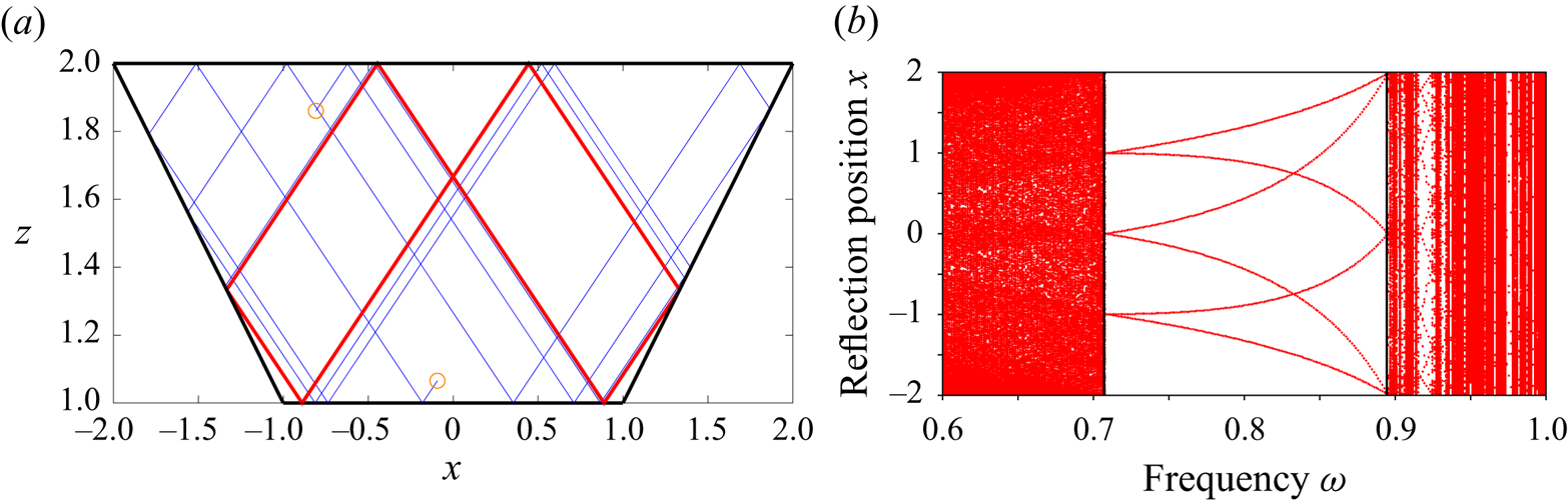
Figure 2. (a) Two-dimensional ray paths for two particular trajectories starting from the orange empty circles and for $\omega =0.8$. The red path corresponds to the last half of the many reflections and shows the final attractor. (b) Position of each reflection along the $x$ axis of the last few reflections as a function of $\omega$. The two vertical lines correspond to $\omega =1/\sqrt {2}$ and $\omega =2/\sqrt {5}$.

If we now authorise the ray beams to deviate from a particular meridional plane, their path becomes more complex. One has to monitor the horizontal angle $\phi$ of the direction of the ray and the meridional angle $\psi$ of the position where it reflects on the boundaries (see figure 6b below). This problem has been recently studied in Pacary et al. (2023) for this particular geometry (see also § 7 in Maas 2005). They showed that the 2-D attractor is still obtained but its location along the azimuthal direction is now dependent on the choice of initial conditions. This phenomenon is illustrated in figure 3, where we show that two rays emitted from the same location with different initial horizontal angles of propagation $\phi$ end on the same 2-D attractor but in different meridional planes. However, the geometry being azimuthally invariant, all the meridional planes are possible and should be obtained with the same probability. A fully axisymmetric attractor would then be obtained (with a non-uniform distribution of trapping planes though, see Maas 2005) if all the possible initial conditions were simultaneously considered (with the exception of whispering gallery modes (Pillet et al. 2019) which we did not observe here). More details can be found in Pacary (2023) and Pacary et al. (2023), where such an axisymmetric system is explored using both ray tracing and experiments.

Figure 3. Ray path for two particular trajectories initialised at the same point indicated by the empty circle. The two trajectories differ only by the initial horizontal angle of propagation. The thin lines correspond to the transient propagation while the thick lines correspond to the final limit cycle after many reflections. The conical surface is coloured in light grey to distinguish it from the horizontal planes. The height of the cone is $H=1$, its opening angle is $\tan \alpha =1$ and the frequency is $\omega =0.8$. (a) Side view. (b) View from the top. A movie (Movie 1) showing the propagation of many randomly initialised rays can be found in the Supplementary materials available at https://doi.org/10.1017/jfm.2024.5.

3.2. Elliptic cone

In this section, we consider the unexplored case $b>1$ in (2.5) which corresponds to a truncated elliptic cone. As the axisymmetry is now broken, we do not expect the presence of any axisymmetric attractor. In the following, we focus on the case where the reflection on the conical surface remains supercritical, which leads to the following upper bound on $b$:

(3.4)\begin{equation} b< b_c=\frac{\tan\alpha}{\tan\theta} . \end{equation}

The first effect of the elliptic deformation is to modify the orientation of the normal vector of the conical surface. Except in the vertical planes $x=0$ and $y=0$ corresponding to the directions of the principal axes of the elliptic cone, the normal vector to the cone is no longer oriented towards the vertical rotation axis. This means that, contrary to the axisymmetric case, no ray can stay trapped in a particular meridional plane apart from the planes $x=0$ and $y=0$. When a ray is initialised inside any other meridional plane, it deviates from it after its first reflection on the conical surface. Whether the planes $x=0$ and $y=0$ are an stable or unstable equilibrium will be discussed below.

We first repeat the ray tracing experiment done previously for $b=1$ but in a non-axisymmetric geometry with $b=1.2$. The same frequency $\omega =0.8$ is considered. An example is shown in figure 4, where two ray paths are generated from the same initial position but with different horizontal angles. We observe that the two ray paths now converge towards the same unique attractor localised in the plane $y=0$ containing the semi-minor axis of the elliptic cone. One can repeat the experiment for many initial positions and horizontal angles $\phi$ showing that all rays eventually end up in this particular plane $y=0$ and along the same limit cycle. For this particular case, it thus seems that the plane $y=0$ is a stable equilibrium while the plane $x=0$ is unstable. This is further confirmed in figure 5, where we show the positions $x$ and $y$ of the reflection points of the limit cycle (obtained by considering the last ten iterations of a total of five hundred) for many frequencies and many random initial conditions. We compare the axisymmetric case $b=1$ in figure 5(a) with the elliptic case $b=1.2$ in figure 5(b). The thin lines indicate the $x$ coordinates of the six reflection points of the 2-D attractor path, as already shown in figure 2(b), in the particular plane $y=0$ which is the same for all ellipticities $b$ in our case. For the axisymmetric case, each independent ray path converges towards a similar 2-D attractor in a particular meridional plane, depending on its initial conditions, leading to a dense pattern of reflection points when plotting their $(x,y)$ coordinates. Note that the projection from the axisymmetric domain to the arbitrary coordinates $x$ and $y$ leads to a non-uniform density of reflection points which tend to accumulate close to the expected positions of the 2-D attractors (shown by the thin lines). For the non-axisymmetric case $b=1.2$, however, all the rays converge towards the particular plane $y=0$, regardless of their initial conditions in terms of position and initial horizontal angle, while we recover the same attractor structure as in two dimensions when considering the $x$ coordinates. Note that we recover this peculiar property for all frequencies within the attractor range given by (3.3).

Figure 4. Same as figure 3 but for a non-axisymmetric domain with $b=1.2$ in (2.5). The other parameters are $\omega =0.8$, $H=1$ and $\tan \alpha =1$. (a) Side view in the $(y,z)$ plane. (b) Side view in the $(x,z)$ plane. (c) Three-dimensional view. (d) Top view in the $(x,y)$ plane. A movie (Movie 2) showing the propagation of many randomly initialised rays can be found in the Supplementary materials available at https://doi.org/10.1017/jfm.2024.5.

Figure 5. Positions of the reflection points along the $x$ axis in red and along the $y$ axis in blue for the final limit cycle obtained from many random initial conditions. (a) Axisymmetric case $b=1$ and (b) elliptic case $b=1.2$. The cone height is $H=1$ and its opening angle is $\tan \alpha =1$. The graph focuses on the frequency range defined by (3.3). The thin lines correspond to the analytical position of the six reflection points of the 2-D attractor.

The attractor in the particular plane $y=0$ seems to attract all the rays, regardless of their initial positions within the volume, with the exception of rays initialised within the $x=0$ plane, which is also an equilibrium, albeit unstable. Contrary to the axisymmetric case, there is a second azimuthal convergence (related to the varying curvature of the elliptic cone along the azimuthal direction) in addition to the meridional convergence at the origin of the classical 2-D attractor (related to the inclination of the conical surface). For this reason, we call this final limit cycle a ‘super-attractor’, to differentiate it from the classical attractor surface observed in the axisymmetric case. The super-attractor results from a convergence of rays in both axial and azimuthal directions while there is no azimuthal convergence for an attractor in an axisymmetric geometry, as its azimuthal position depends on the initial position and horizontal angle of propagation.

3.2.1. Local analysis of the super-attractor

In this section, we analyse the local properties of the super-attractor. Our objective is to confirm the attracting character of the super-attractor both towards a particular limit cycle in the meridional plane and towards a particular meridional plane, regardless of initial conditions. While the first property is shared with regular attractors, we show that the second is specific to super-attractors. We aim to obtain an analytic expression for the attraction rate (i.e. Lyapunov coefficient) as a function of the geometrical parameters.

We focus on the super-attractor which is made of two symmetrical quadrangles, as illustrated in figure 2(a). This 2-D attractor has been studied in § 3.1. It exists in the plane $x=0$ for frequencies in the interval defined in (3.3). The points $(\pm x_a,0,z_a)$ where reflection occurs has been given in (3.1a,b).

We now want to analyse the behaviour of a ray close to the attractor. We consider a ray emitted from a point $(x_0,y_0,z_0)$ on the inclined surface close to $(x_a,0,z_a)$. This ray is emitted downward with a vertical angle $\varphi _0 = {\rm \pi}/2 + \theta$ and an azimuthal angle $\phi _0$ as illustrated in figure 6. If this ray is not too far from the attractor, it first reflects on the lower plane surface, then reflects on the upper plane surface before reaching the inclined surface on the other side in a point $(x_1,y_1,z_1)$ close to $(-x_a,0,z_a)$. Both points $(x_0,y_0,z_0)$ and $(x_1,y_1,z_1)$ are on the cone defined by (2.5) so their horizontal coordinates can be written as

(3.5a)$$\begin{gather} x_0 = z_0 \frac{\cos \psi_0 }{\tan \alpha} ,\quad y_0 = b z_0 \frac{\sin \psi_0 }{\tan \alpha} , \end{gather}$$

(3.5b)$$\begin{gather}x_1 = z_1 \frac{\cos \psi_1 }{\tan \alpha} ,\quad y_1 = b z_1 \frac{\sin \psi_1 }{\tan \alpha} , \end{gather}$$

where $\psi _0$ and $\psi _1$ are their azimuthal angles (see figure 6b).

Figure 6. (a) Perspective view of the elliptic cone in thick solid line. The attractor is indicated by the red line. The cone is twice symmetrically duplicated to avoid considering the reflections on the horizontal planes. (b) View from the top of a ray emitted close to the attractor. The red dashed lines indicate the section of the cone at the altitude $z_a$ of the attractor. The ray emitted from the point $(x_0,y_0,z_0)$ with a horizontal angle $\phi _0$ is reflected at $(x_1,y_1,z_1)$ with the angle $\phi _1$.

As the reflections on the plane surfaces do not modify the azimuthal angle of the ray (see (2.4) for the particular case $\alpha =0$), the coordinates of the point $(x_1,y_1,z_1)$ can be obtained by continuing the ray in horizontal mirror images of the cones. Such a ray reaches the boundary of the second cone image in a point which has just been shifted vertically by twice the height of the cone, that is in $(x_1,y_1,z_1-2H)$ (see figure 6). This property means that there exists $\lambda$ such that

(3.6a)$$\begin{gather} x_1 = x_0 - \lambda \cos \theta \cos \phi_0 , \end{gather}$$

(3.6b)$$\begin{gather}y_1 = y_0 - \lambda \cos \theta \sin \phi_0 , \end{gather}$$

(3.6c)$$\begin{gather}z_1 -2H = z_0 + \lambda \sin\theta . \end{gather}$$

When the ray is close to the attractor, $(x_0,y_0,z_0)$ and $(x_1,y_1,z_1)$ are assumed to be close to $(x_a,0,z_a)$ and $(-x_a,0,z_a)$, respectively. Moreover, $\psi _0$ is assumed to be small, and $\phi _0$ and $\psi _0$ are close to ${\rm \pi}$. At first order, (3.5) give for the relative distances

(3.7a)$$\begin{gather} \delta x_0 \sim \frac{\delta z_0 }{\tan \alpha} ,\quad \delta y_0 \sim b z_a \frac{ \psi_0 }{\tan \alpha} , \end{gather}$$

(3.7b)$$\begin{gather}\delta x_1 \sim{-} \frac{\delta z_1 }{\tan \alpha} ,\quad \delta y_1 \sim{-} b z_a \frac{ (\psi_1 - {\rm \pi}) }{\tan \alpha} . \end{gather}$$

From (3.6c), one gets $\lambda$ as

(3.8)\begin{equation} \lambda \sim \frac{-2H + \delta z_1 -\delta z_0}{\sin\theta}. \end{equation}

Inserting this expression in (3.6a), one obtains, using (3.7a,b), that

(3.9a,b)\begin{equation} \delta x_1 \sim{-} K \delta x_0 ,\quad \delta z_1 \sim K \delta z_0 , \end{equation}

with

(3.10)\begin{equation} K = \frac{\tan \alpha - \tan \theta}{\tan\alpha + \tan \theta} = \frac{\sin(\alpha- \theta)}{\sin(\alpha+\theta)} , \end{equation}

which corresponds to the 2-D contraction factor of the attractor.

In (3.5b), we obtain

(3.11)\begin{equation} \delta y_1 \sim \delta y_0 - \frac{2 H (\phi_0 -{\rm \pi})}{\tan\theta} , \end{equation}

which gives a first relation between the angles

(3.12)\begin{equation} \psi _1 - {\rm \pi}={-}\psi _0 + \frac{2 }{b} (\phi_0 - {\rm \pi}) . \end{equation}

A second relation that expresses the angle $\phi _1$ of the reflected ray in terms of $\phi _0$ and $\psi _0$ is obtained by applying the condition of reflection (2.4) at $(x_1,y_1,z_1)$. Close to the attractor, the azimuthal angle $\phi _{\boldsymbol n}$ of the normal vector ${\boldsymbol n}$ is given at leading order by

(3.13)\begin{equation} \phi_{\boldsymbol n} \sim \frac{(\psi_1 - {\rm \pi})}{b} . \end{equation}

The normal vector ${\boldsymbol n}$ and the incident rays are oppositely oriented with respect to the vertical, so $\zeta ={\rm sgn}(n_z V_{iz}) = -1$. Expression (2.4) then gives, for small angles,

(3.14)\begin{equation} \phi_1 - \phi_{\boldsymbol n} \sim{-}\frac{\tan \alpha - \tan \theta}{\tan\alpha + \tan \theta} (\phi_0 - {\rm \pi}- \phi_{\boldsymbol n}) ={-} K (\phi _0 -{\rm \pi} -\phi_{\boldsymbol n}) . \end{equation}

Using (3.12) and (3.13), this expression finally reduces to

(3.15)\begin{equation} \phi_1 \sim{-}\frac{1+K}{b} \psi_0 + \left(\frac{2(1+K)}{b^2} - K\right) (\phi_0 - {\rm \pi}) . \end{equation}

Expressions (3.12) and (3.15) can be written as

(3.16)\begin{equation} \boldsymbol{\varPsi}_{\!1} = \boldsymbol{\mathcal{M}} \boldsymbol{\varPsi}_{\!0}, \end{equation}

for the vectors $\boldsymbol {\varPsi }_{\!1} = (\psi _1 - {\rm \pi}, \phi _1)^\top$ and $\boldsymbol {\varPsi }_{\!0} = (\psi _0, \phi _0 -{\rm \pi} )^\top$ where the matrix $\boldsymbol {\mathcal {M}}$ is

(3.17)\begin{equation} \boldsymbol{\mathcal{M}} = \left( \begin{array}{cc} -1 & 2/b \\ -(1+K)/b & 2(1+K)/b^2 - K \end{array} \right)\!. \end{equation}

The operation can be repeated and after $2N$ reflections on the cone boundary, that is $N$ cycles, we get

(3.18)\begin{equation} \boldsymbol{\varPsi}_{\!2N} = \boldsymbol{\mathcal{M}}^{2N} \boldsymbol{\varPsi}_{\!0}, \end{equation}

where $\boldsymbol {\varPsi }_{\!2N} = (\psi _{2N}, \phi _{2N} - {\rm \pi})^\top$.

Introducing the eigenvalues $\lambda _{\pm }$ and associated eigenvectors $\boldsymbol {\varPsi }_{\!\pm }$ of the matrix $\boldsymbol {\mathcal {M}}$, which are defined by

(3.19a)$$\begin{gather} \lambda _{{\pm}} = \frac{(1+K)(2/b^2-1) \pm \left((1+K)^2 (2/b^2-1)^2 - 4~K\right)^{1/2}}{2}, \end{gather}$$

(3.19b)$$\begin{gather}\boldsymbol{\varPsi}_{\!\pm} = (2/b, 1 + \lambda_{{\pm}})^\top , \end{gather}$$

$\boldsymbol {\varPsi }_{\!2N}$ can be written as

(3.20)\begin{equation} \boldsymbol{\varPsi}_{\!2N} = C_0 (\lambda _+)^{2N} \boldsymbol{\varPsi}_{\!+} + D_0 (\lambda _-)^{2N} \boldsymbol{\varPsi}_{\!-} , \end{equation}

where $C_0$ and $D_0$ are constants depending on the initial condition only

(3.21a)$$\begin{gather} C_0= \frac{2(\phi_0-{\rm \pi}) - b(1+\lambda_-)\psi_0}{2(\lambda_+ - \lambda_-)} , \end{gather}$$

(3.21b)$$\begin{gather}D_0= \frac{2(\phi_0-{\rm \pi}) - b(1+\lambda_+)\psi_0}{2(\lambda_- - \lambda_+)} . \end{gather}$$

The functions $\lambda _+$ and $\lambda _-$ characterise the behaviour of the angles $\psi _{2N}$ and $\phi _{2N} -{\rm \pi}$ as a function of the cycle number $N$. These angles go to zero if and only if $|\lambda _\pm | <1$. This condition is here equivalent to $b>1$ (since $0< K<1$). The functions $\lambda _{\pm }$ depend on the value of $b$ with respect to the particular values

(3.22)\begin{equation} b_{c\pm} = \frac{\sqrt{2(1+K)}}{1\pm \sqrt{K}} . \end{equation}

The two $\lambda _\pm$ are real positive for $1< b< b_{c+}$, and real negative for $b>b_{c-}$. For $b_{c+}< b< b_{c-}$, they are complex conjugates with a constant absolute values equal to $\sqrt {K}$. When $b=b_{c\pm }$, the solution evolves differently as shown in Appendix B.

3.2.2. Comparison between local analysis and numerical ray tracing

This section compares the prediction of the local analysis with that of the global ray tracing approach described above. To do so, we randomise the initial position inside the volume, the horizontal angle of propagation and the sign of the vertical velocity component. We then track the ray for $10^4$ reflections on boundaries, which is enough to reach the attractor in most cases. The horizontal angle is computed at each reflection on the conical surface and for $x_i>0$ according to $\psi _{i}=\textrm {arg}(x_i+\textrm {i}y_i)=\textrm {atan2}(y_i,x_i)$, where $(x_i,y_i)$ are the coordinates of the $i^{\textrm {th}}$ reflection point on the positive half $x>0$ of the conical surface. The horizontal angle difference $\Delta \psi _i=|\psi _i-\psi _{i-1}|$ is then tracked as a function of the number of cycles. Note that we track the convergence of the horizontal angle after a complete cycle around the attractor for comparison with the prediction (3.19) of the local analysis presented in § 3.2.1. In that case, the analysis is performed on the number of cycles around the attractor and not on the number of reflections on the boundaries (there are 6 reflections on boundaries and 2 reflections on the conical surface per cycle for the particular attractor considered here).

The evolution of the horizontal angle increment is typically characterised by a short transient followed by an exponential decay until machine accuracy is eventually reached and the ray becomes trapped in a particular plane. Some examples for $\omega =0.8$, $H=1$, $\tan \alpha =1$ and three values of $b$ are shown in figure 7(a) to illustrate the convergence process. We observe that all rays converge towards the super-attractor at the same exponential rate, irrespective of the initial conditions. The duration of the transient before the ray effectively converges towards the attractor depends on the initial conditions and corresponds to the early reflections far from the final limit cycle. Note that for this particular case, the particular value of $b$ defined by (3.22) is $b_{c+}=1.097$. Consistent with the theoretical prediction, we observe real values for the decay rate when $b< b_{c+}$ (see the two cases $b=1.02$ and $b=1.05$ in figure 7a) and complex values when $b>b_{c+}$ (see the case $b=1.2$).

Figure 7. (a) Angle difference $\Delta \psi _N= |\psi _N-\psi _{N-1}|$ in logarithmic scale as a function of the number of cycles $N$. We show 100 independent realisations with different initial conditions for each value of $b$. (b) Decay rate $\sigma$ defined by $\Delta \psi _N\sim \exp (\sigma N)$ as a function of the long axis $b$. Symbols correspond to the ray tracing approach while lines correspond to the linear local analysis (3.19). The upper branches correspond to $\sigma = \ln |\lambda _+|$ while the lower branches correspond to $\sigma = \ln |\lambda _-|$. Note that the data for $\omega =0.76$ stop because of the upper bound $b_c\approx 1.17$ as given by (3.4).

A best fit $\Delta \psi _N\sim \exp (\sigma N)$, where $N$ is the number of cycles, is computed in the range $10^{-14}<\Delta \psi _N<10^{-3}$ and averaged over $10^3$ independent rays initialised randomly within the whole volume. Results are shown in figure 7(b). An excellent agreement between the local theoretical prediction and the ray tracing approach is observed for various values of $b$ and three different frequencies within the attractor range. Interestingly, the decay rate is $\sigma =\ln |\lambda _-|=\ln |K|$ when $b=1$ while it is smaller when $b>1$. There is therefore a drastic difference between the case $b=1$, for which all rays converge rapidly toward a plane different for each ray, and the case $b>1$, for which the convergence rate is smaller and actually tends to 0 when $b\rightarrow 1$. Although the breaking of the axisymmetry does create a globally attracting plane, as already discussed previously, the rate of convergence towards this unique plane increases with $b$ and is actually maximum once $b>b_{c+}$. In that case, it is actually half of that observed when $b=1$.

4. Numerical simulations of the linear viscous problem

Up to now, we have only discussed the properties of the ray paths which are only valid in the limit of vanishing Ekman numbers. The link between the properties of the ray paths and the actual viscous solution of the original linear Navier–Stokes equations (2.1) is not obvious. In this context, it is desirable to check whether the globally attracting solutions discussed in previous sections have any counterpart when considering the direct solution of (2.1).

To that end, we solve the linear viscous equations (2.1) using the spectral element solver Nek5000 (Fischer 1997; Deville, Fischer & Mund 2002). The domain is discretised using a number $\mathcal {E}$ of hexahedral elements. Elements have been refined close to all boundaries to properly resolve viscous Ekman layers. The velocity is discretised within each element using Lagrange polynomial interpolants based on tensor-product arrays of Gauss–Lobatto–Legendre quadrature points. The polynomial order $l_d$ of the expansion basis on each element is fixed to $11$ in this study, while the number of elements goes up to $\mathcal {E}=29\,952$ for $E=10^{-7}$. Convergence has been tested by gradually increasing the polynomial order for a fixed number of elements. The Coriolis term is treated explicitly by a third-order extrapolation scheme whereas the viscous terms are treated implicitly by a third-order backward differentiation scheme. Similarly to the ray tracing approach discussed previously, we focus on the particular case $H=1$, $\alpha ={\rm \pi} /4$ and $\omega =0.8$.

Since we want to compare the axisymmetric conical geometry with its elliptic counterpart, care must be taken when choosing the forcing. In particular, latitudinal libration is not well suited since the forcing would be of viscous nature in the axisymmetric case (since the velocity at the boundaries would be purely tangential) while there would be a non-zero normal velocity and hence pressure coupling in the non-axisymmetric elliptic case. Another constraint comes from the corners, which will inevitably contribute to the viscous dynamics by emitting their own singular shear layers. Taking into account these considerations, we opted for a rotating vertical forcing at the bottom plane of the cone, sometimes called negative nutation (Sibgatullin et al. 2017), defined by

(4.1)\begin{equation} u_z(z=1)=\begin{cases} \left(x\cos(\omega t)-y\sin(\omega t)\right)f(r), & \text{if }r<1,\\ 0, & \text{if }r>1, \end{cases} \end{equation}

where $f(r)=2r^3-3r^2+1$ is a smoothing function to ensure that the forcing vanishes close to the corners and $r=\sqrt {x^2+y^2}$ is the cylindrical radius. The other two velocity components are zero and the other boundaries are all no slip. A similar forcing has already been used both experimentally (Pacary et al. 2023) and numerically (Sibgatullin et al. 2019). Note that we obtained qualitatively similar results when considering an axisymmetric forcing similar to that used by Boury et al. (2021) for example.

From a fluid at rest, we run the simulation until a periodic response is obtained. In order to quantify the inhomogeneities between different attractor planes, we first define the 2-D attractor path for each plane obtained from the intersection between a vertical plane containing the origin and the frustum. Each plane is parametrised with its azimuthal angle with respect to the $x$ direction. The plane crossing the short elliptic axis thus corresponds to $\phi =0$ while the plane crossing the long elliptic axis corresponds to $\phi =\pm {\rm \pi}/2$. Note that the 2-D attractor path on each plane depends on the ellipticity $b$. While the same attractor path is expected on each individual plane when $b=1$, different attractors (but the same rectangular topology) are expected when $b>1$. We then compute the averaged velocity amplitude along each path by averaging over time once the periodic response is obtained and along the attractor path. This averaged amplitude is a constant in the axisymmetric case $b=1$ but depends on the orientation of the plane once $b\neq 1$. As we vary the ellipticity of the domain, the amplitude of the response also varies. In order to focus on the azimuthal inhomogeneities induced by the wave attractor, we further normalise the amplitude by its average over all azimuthal angles $\phi$.

This ratio is plotted in figure 8(a) for a fixed $E=10^{-7}$ and varying $b\geq 1$. As expected, it is unity for the axisymmetric case $b=1$. As $b$ increases, a clear focusing of the energy along the short axis corresponding to $\phi =0$ is observed. Note that a second local maximum is also observed along the long axis $\phi =\pm {\rm \pi}/2$. The same simulations are now run at a fixed $b=1.2$ and varying Ekman number from $E=10^{-4}$ down to $E=10^{-7}$. Results are displayed in figure 8(b). While focusing is observed for all Ekman numbers, it is more and more pronounced as the Ekman number decreases. Note again that a residual localisation also persists around the long axis $\phi =\pm {\rm \pi}/2$. This secondary localisation of the energy is not expected from the ray tracing approach only since it corresponds to an unstable equilibrium as discussed previously in § 3.2.1. We have observed such residual localisation strongly depends on the particular choice of forcing and seems to be partially dependent on contributions from the bottom corner (see figure 9b), which goes well beyond our current understanding mostly based on local ray tracing.

Figure 8. Azimuthal profile of the velocity amplitude averaged over time and over the 2-D attractor path on each meridional plane. (a) Variable long axis $b$ at constant Ekman number $E=10^{-7}$. The amplitude is normalised by its azimuthal average. (b) Variable Ekman number at constant long axis $b=1.2$. The forcing frequency is $\omega =0.8$ and the forcing pattern is defined by (4.1) in all cases.

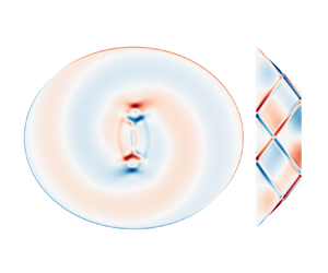
Figure 9. Vertical velocity component in the planes (a) $y=0$, (b) $x=0$ and (c) $z=1.9$. The same colour scale is used for the three plots. Parameters are $E=10^{-7}$, $\omega =0.8$ and $b=1.2$. The inclined line in (a) indicates the profile of the plane shown in figure 10. The dotted lines in (a,b) indicate the plane $z=1.9$ shown in (c) while the dashed lines show the 2-D attractor path in each meridional plane.

A visual inspection of the wave field qualitatively confirms this conclusion. Figure 9 shows the vertical velocity component at a particular time once a periodic response has been obtained. One can see that the response along the attractor path is much stronger in the $y=0$ plane (see figure 9a) than it is in the $x=0$ plane (see figure 9b). Note of course that the 2-D attractor path (shown as dashed lines in figure 9a,b) is not the same in both planes since the domain is non-axisymmetric. This explains why we observe apparently curved wave beams. They correspond to the gradual modification of the attractor path as the geometry changes along the azimuthal direction due to the weak elliptic deformation. Similar structures were for example observed by Bühler & Muller (2007). We also see in figure 9(b) that the attractor path in the unstable plane $x=0$ is very close to the bottom corner, which perhaps explains why we have observed a secondary peak of energy in figure 8. The bottom corner forces a local shear layer which might overlap with the attractor beam in a non-trivial way. Nevertheless, figure 9(c) clearly shows that the amplitude of the stable attractor localised around the plane $y=0$ is significantly larger than that of any other planes, including the unstable attractor localised in the $x=0$ plane.

In order to show the local structure of the super-attractor, we define a plane perpendicular to the attractor path along the short axis, as shown in figure 9(a). The velocity amplitude is averaged over time and normalised by its local maximum closest to the attractor path to obtain the maps displayed in figure 10. We compare the axisymmetric case $b=0$ on the bottom row with the non-axisymmetric case $b=1.2$ on the top row. For the axisymmetric case, one observes the gradual focusing of the axisymmetric wave beam around the attractor position as the Ekman number is decreased. The observed curvature is due to intersection between the flat plane and the curved axisymmetric wave beam. This axisymmetric pattern is clearly broken for $b=1.2$. At $E=10^{-5}$, while we observe a local maximum close to the theoretical position of the super-attractor (which corresponds to the origin with our choice of coordinates), no local beam is observed. At lower Ekman numbers, however, a localised beam is observed with a complex anisotropic structure. It is more elongated along the transverse direction $y$ than along the in-plane coordinate $s$. This confirms that the energy injected by the global large-scale forcing is eventually focused preferentially onto the super-attractor path localised around the $y=0$ plane. While it is too early to convincingly discuss possible scalings with the Ekman number, we nevertheless report the amplitude scaling observed in our simulations in figure 11. We consider three different measures of amplitudes. The first is obtained by averaging over all 2-D attractor paths of each meridional section, which we refer to as global. The second corresponds to the average on the short axis attractor only while the last corresponds to the local amplitude maximum obtained from the maps displayed in figure 10. We observe that, for all three measures, the amplitude increases as the Ekman number decreases. The local measure might follow the scaling $E^{-1/6}$, which is expected from classical 2-D attractors (He et al. 2023) forced by inviscid forcing, although a much larger range of Ekman numbers should be explored to convincingly conclude on this matter. This is left for future works.

Figure 10. Maps of averaged velocity amplitude normalised by its maximum value on the local plane shown in figure 9(a). The Ekman number is decreasing from left to right. The top row (a–c) corresponds to the non-axisymmetric case $b=1.2$ while the bottom row (d–f) corresponds to the axisymmetric case $b=1$. The line shows the iso-contour corresponding to 90 % of the local maximum value around the theoretical attractor location which is the origin of the local frame used here.

Figure 11. Amplitude scaling with Ekman for three different measures: the average is performed over all attractor paths irrespective of their azimuthal orientation (Global), only along the ray path corresponding to the short axis (Short axis) or focusing on the local maximum observed on the maps shown in figure 10 (Local). Note that the local value at $E=10^{-4}$ is absent since we cannot unambiguously measure a local maximum in that case.

5. Discussion

We have shown how a 2-D attractor can be localised in three dimensions into a particular plane by breaking the axisymmetry of the fluid domain. All ray paths have been observed to converge to a particular 1-D curve contained within a specific plane. A local analysis has allowed us to confirm the exponential decay of the horizontal angle and has been successfully compared with ray tracing computations. While numerical simulations have shown a localisation of the energy onto the attracting plane, the harmonic response also contains contributions from the corners which might be at the origin of a secondary peak of energy along the long axis, which is unstable according to our ray tracing analysis. By construction of our particular geometry, the secondary unstable attractor is more and more affected by the corner contributions as $b$ increases, which might explain why we observe a secondary energy increase there. However, the observed increase of kinetic energy along the stable super-attractor can only be explained by a secondary focusing since its topology within the particular plane $y=0$ remains the same regardless of the elliptic deformation $b$.

While our example has convincingly shown the existence of such super-attractors, generalising this result to other geometries would be valuable. We have focused on super-critical reflections only since $\alpha >\theta$ in our case while it is known that the focusing properties of the 3-D reflection is non-trivially depending on the criticality of the slope (Pillet et al. 2019). We suspect that similar super-attractors exist in other conical geometries, including those involving sub-critical slopes, such as those used by Klein et al. (2014), Sibgatullin et al. (2017) and Boury et al. (2021), provided that the axisymmetry used up to now is broken. Other geometries known to support 2-D or axisymmetric attractors, such as the spherical shell or the paraboloidal/parabolic-shaped stadium, can probably generate super-attractors once elliptically deformed. In that respect, much remains to be done to bridge the gap between the local analysis close to the attracting plane and the global properties for which the whole geometry, and not just its asymptotic behaviour close to the attracting plane, matters.

We have considered the particular case of an elliptic deformation in order to break the axisymmetry. While it has the advantage of being a well-defined perturbation of the axisymmetric reference case, it is certainly not the only way to proceed. It would be interesting to consider other types of non-axisymmetric geometries such as cuboids (Wu, Welfert & Lopez 2023). Possible connections with quantum chaos in stadium billiards resulting in scarred patterns could also be explored (Kudrolli, Abraham & Gollub 2001). One could also further investigate the required geometrical properties of the fluid container necessary for the emergence of super-attractors. Finally, it is important to realise that, while the final super-attractor is indeed one-dimensional in the sense that all rays converge towards a 1-D parametric curve, this particular attractor is contained inside a plane since it corresponds to the localisation of the otherwise 2-D attractor. An interesting question would be to know whether general 1-D curves, not necessarily contained within the same plane, can be super-attractors and, if so, in which geometries. This is a tremendous geometrical problem and we hope this preliminary work will motivate future studies in that direction.