Perfect active absorption of water waves in a channel by a dipole source

Abstract

This study investigates the potential use of an active device to efficiently absorb water waves propagating in a channel. The active device comprises a dipole source consisting of two sources in quasi-opposition of phase. We explore the feasibility of this approach to achieve perfect absorption of guided waves through interference phenomena. To accomplish this, we establish the law governing the waves emitted by the dipole source to optimize the absorption of specific incident waves. The validity of this law is demonstrated through numerical simulations and laboratory experiments, encompassing both the harmonic and transient regimes of the experimental set-up.

1. Introduction

The efficient absorption of water waves energy is of prime importance in mitigating their deleterious effects on coastal zones. Addressing and minimizing these impacts pose significant challenges in preserving exposed communities, ecosystems and infrastructure. In pursuit of this objective, passive systems have been proposed, falling into two sub-categories. On the one hand, we find large structures such as artificial reefs, typically constructed using concrete, rock or recycled tires (Sollitt & Cross 1972; van der Meer et al. 2005; van den Brekel 2021; van Gent et al. 2023) or using porous type media, including coastal vegetation, sand dunes or sedimentary layers (Zhu 2001; Silva, Salles & Palacio 2002; Barman & Bora 2021). While these structures can efficiently absorb wave energy, they come at the cost of significant dimensions, of the order of several wavelengths. On the other hand, there are technologies designed for capturing and converting wave energy that may be small in size relative to the wavelength (Salter 1974; Guo & Ringwood 2021; Jin & Greaves 2021). However, they absorb only a small portion of the wave energy, as their primary purpose is energy harvesting rather than the creation of a protected zone.

In contrast to passive absorbers, devices based on active absorption aim to completely cancel outgoing waves from the device. In their classic form, developed over the last sixty years, active absorbers operate by reflection only. They are commonly referred to as ‘absorbing wavemakers’ or ‘reflection compensation systems’ and are employed to generate waves while avoiding undesired reflections, and minimizing disturbances related to artificial boundaries in wave testing facilities. The perfect absorption obtained is made possible by a destructive interference mechanism between the incident wave, whose reflection is to be cancelled, and the wave generated by the active source, i.e. the moving wall hit by the incident wave (Milgram 1965, 1970; Schäffer & Klopman 2000).

In this study, we demonstrate theoretically, numerically and experimentally that a dipole source device can be employed to achieve perfect active absorption of an incident wave in a channel, simultaneously cancelling its reflection and transmission; see figure 1. This device is inspired by the one investigated in Euvé et al. (2023), where perfect passive absorption was achieved using two closely spaced, phase-shifted resonators, whose geometry was carefully tuned for viscous losses and resonance frequency. Here, by actively replicating the absorption conditions observed in that system, we achieve perfect absorption adaptable to any low-frequency incident wave and any loss level. To illustrate the principle of active absorption and its effectiveness, the sections of this paper are structured as follows. The theoretical formulation and numerical validation of the device principle are presented in § 2. The experimental implementation is detailed in § 3, along with an examination of the fields generated solely by the dipole source and the resulting efficient absorption in the harmonic and transient regimes. Brief conclusions are eventually drawn in § 4.

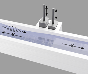
Figure 1. Perfect absorption by a dipole source. (a) Schematic view of the experimental set-up. (b) Experimental realization of the dipole source producing asymmetric wave propagation in the guide. The waves are visualized by a black line projected onto the free surface of the water, made diffusive by a white dye.

2. Perfect absorption: modelling and numerical validation

We consider the propagation of water waves within a channel characterized by width $d$ and water depth $h$. The channel contains two extended sources positioned along one of its vertical walls, forming a dipole source that induces inflows/outflows into the channel. The two sources, rectangular and identical, have horizontal and vertical dimensions $(a, b)$, with their centres submerged at depth $h_{o}$ and spaced along the $x$-axis at a distance $e$. Our modelling approach begins with the full three-dimensional (3-D) problem set in $\varOmega =\{x\in (-\infty,+\infty ),y\in (0,d),z\in (-h,0)\}$, with the origin at the mean free surface, and $z$ directed vertically upwards. Assuming an inviscid, incompressible fluid and irrotational motion, the velocity potential $\phi (\boldsymbol {r},t)$ and associated velocity $\boldsymbol {u}(\boldsymbol {r},t)$ satisfy

(2.1) \begin{equation} \text{3-D problem} \quad \left\{\begin{array}{@{}l} \displaystyle \boldsymbol{u}=\boldsymbol{\nabla} \phi,\quad \boldsymbol{\nabla}\boldsymbol{\cdot} \boldsymbol{u}=0,\quad\text{in } \varOmega, \\ \displaystyle {u_z}_{|z=0}=-\dfrac{1}{g}\,\dfrac{\partial^2 \phi}{\partial t^2}_{|z=0},\quad\displaystyle {u_z}_{|z=-h}=0, \\ \displaystyle {u_y}_{|\varGamma}=0,\quad{u_y}_{|\varGamma_i}=U_i, \quad i=1,2, \end{array}\right. \end{equation}

where $g$ is the gravitational constant, $t$ is time, and $\boldsymbol {r}=(x,y,z)$. We have defined the surfaces $\varGamma _i$, $i=1,2$, and $\varGamma$ as

(2.2)\begin{equation} \left.\begin{gathered} \varGamma_1=\{(x+e/2)\in(-a/2,a/2), y=d, (z-h_{o})\in(-b/2,b/2)\},\\ \varGamma_2=\{(x-e/2)\in(-a/2,a/2), y=d, (z-h_{o})\in(-b/2,b/2)\},\\ \varGamma=\{x\in(-\infty,\infty),y\in\{0,d\},z\in(-h,0)\}\setminus (\varGamma_1\cup\varGamma_2), \end{gathered}\right\} \end{equation}

which correspond respectively to the regions of the vertical walls occupied by the two sources and the rigid regions of the vertical walls.

2.1. Reduction of the model: the two-dimensional problem

In the harmonic regime with time dependence ${\rm e}^{-{\rm i}\omega t}$, we go from the 3-D problem to a two-dimensional (2-D) reduced problem. To achieve this, we employ the modal representation of the 3-D solution

(2.3)\begin{equation} \phi(\boldsymbol{r},t)={\rm e}^{-{\rm i}\omega t}\sum_{n\geq 0}\varphi_n(x,y)\,f_n(z), \end{equation}

where

(2.4a,b)\begin{equation} f_n(z)=\frac{\cosh k_n(z+h)}{\cosh k_nh}, \quad k_n\tanh k_n h=\frac{\omega^2}{g}, \end{equation}

such that

(2.5a,b)\begin{equation} \int_{-h}^0 f_m(z)\,f_n(z)\,{\text{d}} z=N_n\delta_{mn},\quad N_n=\frac{\sinh (2k_nh)+2k_nh}{4k_n\cosh^2(k_nh)}. \end{equation}

Rearranging (2.3) into (2.1) and projecting onto $f_0(z)$ results in a 2-D problem satisfied by $\varphi (x,y)=\varphi _0(x,y)$ in $\varSigma =\{x\in (-\infty,+\infty ),y\in (0,d)\}$ (and we also note $k=k_0$ as the real-valued wavenumber of the propagating water waves) of the form

(2.6)\begin{equation} \text{2-D problem}\quad \left\{\begin{array}{@{}l} \displaystyle \Delta \varphi +k^2\varphi=0,\quad\text{in } \varSigma, \\ \displaystyle\dfrac{\partial{\varphi}}{\partial{y}}_{|\gamma}=0,\quad\displaystyle \dfrac{\partial{\varphi}}{\partial{y}}_{|\gamma_i}=u_i, \quad i=1,2, \end{array}\right. \end{equation}

where

(2.7)\begin{equation} \left.\begin{gathered} \gamma_1=\{(x+e/2)\in(-a/2,a/2), y=d\}, \quad \gamma_2=\{(x-e/2)\in(-a/2,a/2), y=d\}, \\ \gamma=\{x\in(-\infty,\infty),y\in\{0,d\}\}\setminus (\gamma_1\cup\gamma_2), \end{gathered}\right\} \end{equation}

and

(2.8a,b)\begin{equation} u_i=\alpha U_i,\quad \alpha = \frac{8\cosh(kh)\cosh(k(h-h_{o}))\sinh(kb/2)}{\sinh(2kh)+2kh}. \end{equation}

We consider an incident wave propagating to the right, characterized by a complex amplitude $\varphi _{inc}$ and sufficiently low frequency such that $k d< 2{\rm \pi}$, implying that only one mode, independent of $y$, is propagating in the 2-D guide. Accordingly, the solution of (2.6) away from the dipole source takes the form

(2.9)\begin{equation} \left.\begin{array}{ll@{}} \varphi(x,y)\simeq \varphi_{inc}\,{\rm e}^{{\rm i}k x}+\varphi^{-}\,{\rm e}^{-{\rm i}k x}, & x\to -\infty,\\ \varphi(x,y)\simeq \varphi^+\,{\rm e}^{{\rm i}k x}, & x\to +\infty, \end{array}\right\} \end{equation}

where $\varphi ^{-}$ and $\varphi ^+$ represent the complex amplitudes of left and right outgoing waves, respectively. The 2-D problem (2.6) can be solved explicitly. In particular, simple expressions for $(\varphi ^{-},\varphi ^+)$ in (2.9) are obtained through Green's identity, as elaborated in Appendix A. They read

(2.10)\begin{equation} \left.\begin{array}{@{}c@{}} \displaystyle \varphi^{-}= \dfrac{{\rm i}\sin(ka/2)}{k^2d}\left(u_1\,{\rm e}^{-{\rm i}ke/2}+u_2\,{\rm e}^{{\rm i}ke/2}\right),\\ \displaystyle \varphi^+=\varphi_{inc}+\varphi^+_0,\quad \varphi^+_0= \dfrac{{\rm i}\sin(ka/2)}{k^2d}\left(u_1\,{\rm e}^{{\rm i}ke/2}+u_2\,{\rm e}^{-{\rm i}ke/2}\right). \end{array}\right\} \end{equation}

We will now establish the conditions on $(u_1,u_2)$ necessary to achieve perfect absorption of the incident wave, i.e. to ensure that $\varphi ^{-}=\varphi ^+=0$. We can already note a specific scenario when $ka=2n{\rm \pi}$, where $n$ is an integer, and $kd<{\rm \pi}$. In this case, $\varphi ^{-}=\varphi ^+_0=0$ regardless of the value of $\varphi _{inc}$ and the values of $u_1$ and $u_2$. These solutions satisfy $\varphi \to 0$ as $x\to \pm \infty$ with $\partial _y\varphi$ remaining constant along $\gamma _i$, where $i=1$ or 2, and they are associated with the superposition of two localized eigenmodes; see Appendix B. Note that this particular scenario renders the sources inactive regarding the incident wave, with $\varphi ^{-}=0$ and $\varphi ^+=\varphi _{inc}$ whatever the values of $(u_1,u_2)$. Then for $ka\neq 2 n{\rm \pi}$, $\varphi ^{-}=0$ is obtained from (2.10) if $(u_1,u_2)$ satisfy the relation

(2.11)\begin{equation} u_2=-u_1\,{\rm e}^{-{\rm i}k e}, \end{equation}

which remains valid regardless of the presence or absence of an incoming wave in the guide. Subsequently, in the presence of an incoming wave and when the above condition is met, $\varphi ^+=0$ is possible if condition

(2.12)\begin{equation} u_1=\frac{k^2d }{2\sin (ka/2) \sin (k e)}\,{\rm e}^{{\rm i}k e/2}\,\varphi_{inc} \end{equation}

is also satisfied. Once again, we notice a specific scenario when $ke=n{\rm \pi}$, where $n$ is an integer. In these cases, the solutions satisfy $\varphi \to 0$ as $x\to \pm \infty$ and either (i) $\partial _y\varphi =C$ along $\gamma _1$, and $\partial _y\varphi =-C$ along $\gamma _2$, or (ii) $\partial _y\varphi =C$ along $\gamma _1$ and $\gamma _2$, where $C$ is a constant. Similar to the previous scenario, these solutions are associated with localized eigenmodes (see Appendix B) and inactive sources with $\varphi ^{-}=0$ and $\varphi ^+=\varphi _{inc}$.

2.2. Numerical validation of the model

In this subsection, we inspect the validity of the model by comparisons with direct numerics. The numerical computations are performed using the PDE tool in Matlab, which employs the finite element method to solve partial differential equations. We consider the geometry depicted in figure 2, and apply radiation conditions at the ends of the guide $x=\pm x_{M}$, consistent with (2.9) for $x_{M}\gg (a+e)/2$. Specifically, we impose $\partial _x\varphi + \textrm {i}k\varphi =2\textrm {i}k\varphi _{inc}\,\textrm {e}^{\textrm {i}kx_{M}}$ at $x=-x_{M}$, and $\partial _x\varphi - \textrm {i}k\varphi =0$ at $x=x_{M}$, consistent with (2.9).

Figure 2. The two-dimensional reduced problem with extended sources considered in the numerics.

To begin with, we consider the amplitudes $(\varphi ^{-},\varphi ^+_0)$ generated solely by the sources; in the model, they are determined by (2.10) with $\varphi _{inc}=0$. Figure 3 shows the variations of these quantities, normalized to $(au_1)$, against the phase and amplitude of $(u_2/u_1)$, from direct numerics (figures 3a,b) and from the model, (2.10) (figures 3c,d). The agreement between the two sets of results is excellent, showing a relative discrepancy of only 0.1 % (we have considered $kd={\rm \pi} /2$, $ka={\rm \pi} /4$ and $ke={\rm \pi} /4$). Numerically, this representation for $\varphi _{inc}=0$ is sufficient to determine the couple $(u_1,u_2)$ capable of achieving perfect absorption $\varphi ^{-}=\varphi ^+=0$. We begin by determining $\xi =u_2/u_1$ that yields $\varphi ^{-}=0$, since this condition is independent of the value of $\varphi _{inc}$. In figure 3, $\varphi ^{-}=0$ is obtained for $\xi =\textrm {e}^{2.36\textrm {i}}$ (white cross), aligning well with (2.11). We then determine the value of $\chi =-\varphi ^+_0/(au_1)$ for $u_2/u_1=\xi$. Eventually, in the presence of any incident wave $\varphi _{inc}$, the condition $\varphi ^+=0$ is obtained simply by linearity when $\varphi _{inc}/(au_1)=\chi$. In the case reported in figure 3, we obtain $\chi \simeq 0.44\,\textrm {e}^{-0.4\textrm {i}}$, demonstrating again good agreement with the model; see (2.12). We notice that in practice, for any incident wave $\varphi _{inc}$, perfect absorption is achieved by imposing

(2.13a,b)\begin{equation} u_1=\frac{\varphi_{inc}}{a\chi},\quad u_2=\xi u_1. \end{equation}

Figure 3. Validation of the model – wave amplitudes of the outgoing waves $(\varphi ^{-},\varphi ^+)$ normalized to $(a u_1)$ as a function of the source amplitude ratio $u_2/u_1$ (modulus and phase) obtained numerically and theoretically for $\varphi _{inc}=0$. The white crosses indicate the theoretical prediction for $\varphi ^{-}=0$ from (2.11). The parameters are $kd={\rm \pi} /2$, $ka={\rm \pi} /4$ and $ke={\rm \pi} /4$.

The above relations involve $(\xi,\chi )$, which depend on the frequency and on the geometry of the guide through $(ka,ke, kd)$. Numerically, they are determined from the analysis of representations as those of figure 3; theoretically, they are given by

(2.14a,b)\begin{equation} \xi=-{\rm e}^{-{\rm i}ke},\quad \chi=\frac{2\sin (ka/2)\sin(ke)}{k^2 ad}\,{\rm e}^{-{\rm i}ke/2}. \end{equation}

Results in figure 4 showcase variations of $(\xi,\chi )$ determined numerically as a function the non-dimensional distance between the two sources $ke \in (0,2{\rm \pi} )$ (with $kd={\rm \pi} /2$ and $ka={\rm \pi} /4$), the source extension $ka \in (0,2.5{\rm \pi} )$ (with $kd={\rm \pi} /2$ and $ke=2.5{\rm \pi}$), and the channel width $kd \in (0,{\rm \pi} )$ (with $ka={\rm \pi} /4$ and $ke={\rm \pi} /4$). The theoretical predictions (2.13a,b) are represented by solid lines for comparison, showing excellent agreement over large ranges of the parameters. It is noteworthy that for small $ke$, implying small $ka$ (figure 4a), the two sources producing perfect absorption are nearly in phase opposition, hence they indeed behave as a dipole source. We also encounter the specific scenarios of inactive sources $\varphi ^{-}=\varphi ^+_0=0$, hence $\varphi _{inc}=0$, for $ke={\rm \pi}$ or for $ka=2{\rm \pi}$.

Figure 4. Numerical results – influence of the geometry on the conditions for perfect absorption. Source amplitude ratio $\xi =u_2/u_1$ (modulus and phase) and relative incident wave amplitude $\chi =\varphi _{inc}/(a u_1)$ (modulus and phase) against the geometrical parameters: (a,b) the distance between the sources $ke$ (fixing $kd={\rm \pi} /2$ and $ka={\rm \pi} /4$); (c,d) the source size $ka$ ($kd={\rm \pi} /2$ and $ke=2.5{\rm \pi}$); and (e,f) the channel width $kd$ ($ka={\rm \pi} /4$ and $ke={\rm \pi} /4$). The markers correspond to the numerical results, and the curves to the theoretical model.

3. Experimental realization of the active absorption

In our experiments, we use a channel with width $d=50$ mm and length 1.2 m, maintaining a fixed water depth $h=26$ mm. The dipole source is implemented by drilling two submerged openings on one of the vertical walls of the channel, each opening having width $a=20$ mm and height $b =10$ mm. The two openings are separated by a distance 5 mm (hence $e=25$ mm) and placed at depth $h_o=16$ mm (see figure 1). Each opening is connected to a cavity producing a controlled flux through its horizontal surface $S_p=19\times 19\ \textrm {{mm}}^2$, with the flux created by the vertical motions of a rectangular piston with the same surface area, and controlled by a linear motor.

We measure the fields of the free surface elevation $\hat {\eta }(x,y,t)$ using an optical method known as Fourier transform profilometry (Cobelli et al. 2009; Maurel et al. 2009). This method relies on acquiring and analysing the fringe patterns projected onto the water surface, with the water rendered diffusive by the addition of a dye (Przadka et al. 2012). Eventually, reflections at the free ends of the channel are minimized by using 5-degree sloping beaches. In scenarios without an incident wave in the channel ($\eta _{inc}=0$), two beaches are positioned at the left and right ends of the channel. In the presence of an incident wave generated by a wavemaker at the left end of the channel, a single beach is used (at the right end of the channel).

3.1. Active absorption in the harmonic regime

In the harmonic regime, we proceed by controlling the two pistons independently at frequency $\omega$ and amplitudes $p_1$ and $p_2$. The conservation of fluxes implies that the mean velocities $U_n$, where $n=1,2$, satisfy $-\textrm {i}\omega p_nS_p=ab U_n$. Consequently, from (2.8a,b) the velocities $u_n$ used in the 2-D model are given approximatively by

(3.1)\begin{equation} u_n=-{\rm i}\alpha \omega\,\frac{S_p}{ab}\,p_n,\quad n=1,2, \end{equation}

with $\alpha$ defined in (2.8a,b). Next, the measured field of the free surface elevation $\hat \eta (x,y,t)$ provides $\eta (x,y)$ by Fourier transform, namely

(3.2)\begin{equation} \eta(x,y)=\frac{1}{T}\int_{0}^T \hat \eta(x,y,t) \,{\rm e}^{{\rm i}\omega t}\,{\text{d}} t, \end{equation}

with $T$ covering several periods (typically 20), and we now seek solutions in the far field of the form

(3.3)\begin{equation} \left.\begin{array}{ll@{}} \eta(x,y)\simeq \eta_{inc}\,{\rm e}^{{\rm i}k x}+\eta^-\,{\rm e}^{-{\rm i}k x}, & x\to -\infty,\\ \eta(x,y)\simeq \eta^+\,{\rm e}^{{\rm i}k x}, & x\to +\infty, \end{array}\right\} \end{equation}

as in (2.9). With $\hat \eta (x,y,t)=-(1/g)\,\partial _t\phi (x,y,0,t)$, and utilizing (2.3), (2.10) and (3.1), the complex amplitudes $(\eta ^-,\eta ^+)$ can be written as

(3.4)\begin{equation} \left.\begin{array}{@{}c@{}} \eta^-= {\rm i}\beta \left(p_1\,{\rm e}^{-{\rm i}ke/2}+p_2\,{\rm e}^{{\rm i}ke/2}\right),\\ \eta^+=\eta_{inc}+\eta^+_0,\quad \eta^+_0={\rm i}\beta\left(p_1\,{\rm e}^{{\rm i}ke/2}+p_2\,{\rm e}^{-{\rm i}ke/2}\right), \end{array}\right\} \end{equation}

with $\beta$ a non-dimensional parameter defined by

(3.5)\begin{equation} \beta= \frac{\omega^2}{g}\,\frac{S_p}{ab}\,\frac{\sin(ka/2)}{k^2d}\, \alpha. \end{equation}

Accordingly, the conditions for perfect absorption read

(3.6a,b)\begin{equation} p_1=\frac{\eta_{inc}}{\chi_{e}},\quad p_2=\xi p_1, \end{equation}

which is the equivalent of (2.13a,b), with $\xi =-\textrm {e}^{-\textrm {i}ke}$ and $\chi _{e}=2\beta \sin (ke)\,\textrm {e}^{-\textrm {i}ke/2}$.

In our first experiments, we follow the same procedure as in our numerical simulations, using $\eta _{inc}=0$, and measure the waves $\eta (x,y)$ generated by the dipole source in the harmonic regime. Following (2.13a,b), we aim to find the condition $p_2=\xi p _1$ capable of experimentally producing $\eta ^-=0$ and characterize the corresponding values of $\chi _{e}=-\eta ^+_0/p_1$. To achieve this, we set the frequency to $\omega =14.5\ \textrm {rad}\ \textrm {s}^{-1}$, corresponding to $kd\simeq {\rm \pi}/2$, and conduct a series of $11\times 21$ experiments with varying $(p_1,p_2)$. The typical amplitude of each piston is $p_n\sim 5$ mm. Specifically, we consider 11 values of $|p_2/p_1|\in (0, 2)$, and for each modulus ratio, we vary the relative phase of $(p_2/p_1)$ between $-{\rm \pi}$ and ${\rm \pi}$ with a step of ${\rm \pi} /20$. In each experiment, we measure the entire field $\eta (x,y)$, and by averaging it over $y$ in the far field (sufficiently distant from the source), we determine the constant complex amplitudes $(\eta ^-,\eta ^+_0)$. The results, depicted in figure 5, demonstrate good agreement with the theoretical model in (3.4). In particular, the agreement confirms (see white crosses in figure 5) that for $p_2/p_1=\xi =-1.03\,\textrm {e}^{-\textrm {i}0.75}\simeq -\textrm {e}^{-\textrm {i}ke}$, the left-outgoing wave vanishes ($\eta ^-\simeq 0$), and the corresponding value $\chi _{e}=-\eta ^+_0/p_1= 0.13\,\textrm {e}^{-\textrm {i}0.36}$ is consistent with (3.4).

Figure 5. Amplitudes of the outgoing waves ($\eta ^-,\eta ^+_0$) normalized to $p_1$ as a function of the ratio $p_2/p_1$ (modulus and phase) obtained experimentally and theoretically (see (3.4)) for $\eta _{inc}=0$. The white crosses indicate the theoretical prediction for $\eta ^-=0$. The frequency is $\omega =14.5\ \textrm {rad}\ \textrm {s}^{-1}$ ($kd\simeq {\rm \pi}/2$).

In the next step, we quantitatively characterize the condition for perfect absorption across frequencies. Specifically, we vary the frequency within the range such that $k\in (0.2,0.7){\rm \pi} /d$ and conduct a coarse version of the analysis depicted in figure 5, employing only $3\times 3$ experiments centred on the theoretical value $p_2/p_1=-\textrm {e}^{-\textrm {i}ke}$, resulting in $\eta ^-=0$. This is done by selecting $|p_2/p_1|$ from the set $\{0.9,1,1.1\}$, and the phase of $(p_2/p_1)$ from $-ke+{\rm \pi} \{0.96,1,1.04\}$; afterwards, linear interpolations are employed to determine the optimal condition for achieving perfect absorption. By repeating this experimental procedure four times, we obtained a refined mean prediction along with error bars derived from standard deviations. The conditions for perfect absorption are depicted in figure 6, illustrating $\xi =p_2/p_1$ (both modulus and phase), yielding $\eta ^-=0$, and the corresponding values of $\chi _{e}=\eta _{inc}/p_1=-\eta ^+_0/p_1$ across various frequencies. To compare with the model (3.6a,b) represented by solid lines in figure 6), $\xi$ and $\chi _{e}$ were calculated using complex wavenumbers $k\to k+\textrm {i}k_{im}$, where the small imaginary part $k_{im}=2\times 10^{-2}\,k^2d$ accounts for attenuation due to viscous losses. This function fits the losses observed experimentally.

Figure 6. Experimental measurements – conditions for perfect absorption. Source amplitude ratio $\xi =p_2/p_1$ (modulus and phase) and relative incident wave amplitude $\chi _{e}=\eta _{inc}/p_1=-\eta ^+_0/p_1$ (modulus and phase) against the frequency by means of $kd$. The markers correspond to the experimental measurements, and the curves to the theoretical model (3.4), in which complex wavenumbers with a small imaginary part $k_{im}=2\times 10^{-2}\,k^2d$ were used to account for attenuation, due to viscous losses.

Eventually, figure 7 presents experimental evidence of perfect absorption when $\eta _{inc}\neq 0$. We generated $\eta _{inc}$ at $\omega =12.6\ \textrm {rad}\ \textrm {s}^{-1}$ ($kd=0.42{\rm \pi}$) using a plunging-type wavemaker placed at the left end of the waveguide and controlled by a linear motor. The complex amplitude $\eta _{inc}$ was characterized in a preliminary study (not reported), in the absence of dipolar source ($\,p_1=p_2=0$). This allowed us to determine the complex amplitudes $(p_1,p_2)$ producing perfect absorption, according to (3.6a,b), which was validated in figure 6. In practice, generating the incident waves and those emitted by the dipole source is achieved by synchronizing the three linear motors. Figure 7(a) displays the corresponding $\eta (x,y)$ (real part) derived from the measured field $\hat {\eta }(x,y,t)$ using (3.2). For comparison, figure 7(b) presents the result obtained via numerical computation in two dimensions under the same conditions. The profile of $\eta$ along $x$ reported in figure 7(c) represents an average of $\eta (x,y)$ over $y$. It reveals weak outgoing waves, with $\eta ^+$ approaching zero for $x\gtrsim 2a$, and $\eta$ without the characteristic beatings indicative of the superposition of left- and right-going waves for $x\lesssim -2a$, hence $\eta ^-\sim 0$. To further quantify the smallness of $\eta ^-$ and $\eta ^+$, fits of $\eta$ were conducted for $x$ in the ranges $(-0.4,-0.05)$ cm and $(0.05,0.4)$ cm, utilizing $k_{im}=2\times 10^{-2}\,k^2d$ as done previously. This procedure was repeated for 11 frequencies corresponding to $kd$ in the range $(0.2, 0.7){\rm \pi}$. The results of this series of experiments are presented in figure 7(d), confirming consistent absorption efficiency with $(|\eta ^-/\eta _{inc}|^2+|\eta ^+/\eta _{inc}|^2)$ at approximately $10^{-3}$ over the entire frequency range, signifying 99.9 % absorption.

Figure 7. (a) Real part of $\eta (x,y)$ measured experimentally, for $\omega =12.6\ \textrm {rad}\ \textrm {s}^{-1}$ (corresponding to an incident wavenumber $kd/{\rm \pi} =0.42$). (b) Same results from direct numerics. (c) Average in $y$ of $\eta (x,y)$. (d) Left-going and right-going energies, normalized to the incident one, against the incident wavenumber $kd/{\rm \pi}$.

3.2. Active absorption in the transient regime

To conclude our experimental demonstration of perfect absorption, we investigate an incoming wave signal in the transient regime. This signal is generated based on its Fourier transform $\eta _{inc}(\omega )$, randomly distributed in phase and modulus but constrained by a Gaussian profile, specifically

(3.7)\begin{equation} \left.\begin{gathered} \eta_{inc}(\omega) \ \text{random with } |\eta_{inc}(\omega)|<\eta_0\exp\left({-\frac{(\omega-\omega_0)^2}{\sigma^2}}\right),\\ \hat{\eta}_{inc}(x,t)=\int_0^{\infty} \eta_{inc} (\omega)\exp({{\rm i}(kx-\omega t)})\,\text{d}\omega, \end{gathered}\right\}\end{equation}

with parameters $\eta _0=0.08$ mm, $\omega _0=14.5\ \textrm {rad}\ \textrm {s}^{-1}$ and $\sigma =4\ \textrm {rad} \textrm {s}^{-1}$ (see figure 8e). In practice, we consider $N=100$ discrete frequencies $\omega _i\in (1,30)\ \textrm {rad}\ \textrm {s}^{-1}$. Leveraging our earlier study in the harmonic regime, where we identified $\eta _{inc} (\omega )/p_1(\omega )$ and $p_2(\omega )/p_1(\omega )$ for perfect absorption (figure 6 and (3.6a,b)), we generate $\hat {p}_1(t)$ and $\hat {p}_2(t)$ through Fourier transforms.

Figure 8. (a) Space–time diagram $\eta (x,t)$, average in $y$ of $\eta (x,y,t)$, reporting the propagation of an incident wave generated following (3.6a,b) and its interaction with the dipole source tuned to achieve perfect absorption. (b) Time signal before (at $x=-0.2$ m) and after (at $x=0.2$ m) the dipolar source. (c,d) Space and time Fourier transforms ${\lvert }{\hat {\eta }(k,\omega )}{\rvert }$ calculated for $x<0$ and $x>0$, revealing vanishing outgoing waves, all the energy corresponding to the incident wave $\eta _{inc}$ in alignment with the theoretical dispersion (black line in c). (e) Wave amplitude along the dispersion relation of the incident and outgoing waves.

The primary result is presented in figure 8(a), which illustrates a space–time diagram of the signal $\hat {\eta }(x,t)$ averaged over $y\in (0,d)$. The effective absorption attributable to the dipole source centred at $x=0$ is evident. Indeed, $\hat {\eta }(x,t)$ remains constant in shape over time for any $x\lesssim -2a$ up to slight attenuation during propagation, while it is nearly zero for $x\gtrsim 2a$. These characteristic shapes are illustrated for $x=-0.2$ m and $x=0.2$ m in figure 8(b). To evaluate absorption quantitatively, we analyse the amplitudes in Fourier space ${{\eta }(k,\omega )}$ in these two regions utilizing

(3.8)\begin{equation} \eta^\pm(k,\omega)=\int_{x_{1}^\pm}^{x_{2}^\pm}\int_{0}^{T} \hat{\eta}(x,t)\exp({{\rm i}(\omega t -kx)})\,{\text{d}}\kern0.06em x\,{\text{d}} t, \end{equation}

with $T=20$ s, $(x_{1}^-,x_{2}^-)=(-0.4\ \textrm {m}, 0)$ and $(x_{1}^+,x_{2}^+)=(0, 0.4\ \textrm {m})$ (before and after the dipole). Results in the $(k,\omega )$ plane are shown in figures 8(c) and 8(d), respectively. In figure 8(c), it is notable that the spectral content of $\eta ^-(k,\omega )$ is almost zero for $k<0$, particularly along the dispersion line $k=-k(\omega )$ (solid red line), and lies predominantly along the dispersion line $k=k(\omega )>0$ (solid black line), hence associated with the right-going wave only. This confirms $\eta ^-=0$. Similarly, figure 8(d) demonstrates that the spectral content of $\eta ^+(k,\omega )$ along the line $k=k(\omega )$ is nearly zero. The amplitude along each dispersion line is shown in figure 8(e). These observations are further quantified by deriving a measure of the energy of the incident, left-going and right-going waves by calculating the energies along these lines, namely

(3.9)\begin{equation} \left.\begin{gathered} E_{inc}=\int_0^{2\omega_0}{\lvert}{{\eta}^-(+k(\omega),\omega)}{\rvert}^2 \,\text{d}\omega,\quad E^-=\int_0^{2\omega_0}{\lvert}{{\eta}^-(-k(\omega),\omega)}{\rvert}^2 \,\text{d}\omega,\\ E^+=\int_0^{2\omega_0}{\lvert}{{\eta}^+(+k(\omega),\omega)}{\rvert}^2 \,\text{d}\omega, \end{gathered}\right\} \end{equation}

resulting in an absorption $(E_{inc}-E^--E^+)/E_{inc}=99.5\,\%$.

4. Concluding remarks

The active absorption device that we have proposed is inspired by two absorption systems. First, it takes up the concept of conventional active absorption, which traditionally works only in reflection, and is extended here to encompass both reflection and transmission, independently of viscous losses. Second, it is inspired by a passive device for which we had demonstrated a relationship between the amplitudes of the resonators and that of the incident wave leading to perfect absorption (Euvé et al. 2023). We have adopted this relationship in the active system, thus avoiding dependence on the level of loss and extending its range of frequency validity. This has been demonstrated for waves guided in a channel. It should be noted, however, that following the developments proposed for active absorbers in reflection in Schäffer & Klopman (2000), our absorber should be applicable to unguided configurations and arbitrary incidences.