Analytical results for pitching kinematics and propulsion performance of flexible foil

Abstract

Natural flyers and swimmers employ flexible wings or fins to propel. While the complex interaction between the foil with deformation and the surrounding non-steady fluid environment defines the propulsion performance of the propellers, elucidating the interaction mechanism through theoretical models earns much challenge. Based on elastokinetics and linear potential flow theory, this study proposes a simplified analytical model to clarify the kinematics and the propulsion performance of a flexible thin foil pitching in flow. The dynamical forces, including the inertial force of the foil and the non-steady fluid pressure, are used to determine the averaged deformation angle of the foil. Combining the averaged deformation angle and the prescribed driving pitching motion, the kinematics of the foil is resolved analytically. Based on the analytical expressions for the corresponding pitching motion, analytical relations among the physical parameters of the stiffness and the mass of the foil and the driving frequency are given to these critical conditions, including resonance of the flow–structure system, equal pitching amplitude between the flexible foil and the rigid counterpart, phase angle transition from ${\rm \pi}/2$ to $- {\rm \pi}/2$. Subsequently, the performance of the foil, including the thrust, the power and the propulsive efficiency, as a function of the flexibility of the foil are derived, together with the introduction of a bluff body type offset drag to the thrust. The formulated analytical theory, which matches nicely with previous reports, will help to interpret the effect of the flexibility and regulate the propulsive performance of the flexible foil when pitching in fluid.

1. Introduction

Natural flyers and swimmers employ the complex interaction between the foils and the surrounding fluid to generate sufficient thrust to locomotion, where the deformation of the flexible foil adds new challenges to the flow–structure interaction. Thus, a vast number of investigations from various aspects have been deployed to reveal the mechanism of the interaction between the flexible foil and the fluid, such as from active and passive foil deformation (Tytell et al. 2010; Flammang & Lauder 2013; Ulrich & Peters 2014; Joshi & Bhattacharya 2022), from localized and distributed flexibility (Shahzad et al. 2018; Shi, Xiao & Zhu 2020; Wang, Huang & Lu 2020; Kurt, Mivehchi & Moored 2021; Wang et al. 2021; Demirer et al. 2022), from tethered and unconstrained motion (Arora et al. 2018; Lin, Wu & Zhang 2020; Fernandez-Feria, Sanmiguel-Rojas & Lopez-Tello 2022; Wu et al. 2022) and from vortical structures and their interactions (Eldredge & Jones 2019; Linehan & Mohseni 2020; Jia et al. 2021; Zhang et al. 2021; Verma & Hemmati 2022). Among these investigations, elucidating the propulsive performance of the flexible foil earns much attention as this will not only help to unveil the flight or swimming mechanism (Wu 2011; Gazzola, Argentina & Mahadevan 2014; Sun 2014; Lauder 2015; Chin & Lentink 2016; Saadat et al. 2017; Dabiri 2019; Wang et al. 2022), it will also help to optimize the manmade flying vehicles and swimming robotics through flapping propulsion (Karasek et al. 2018; Zhu et al. 2019; Chin et al. 2020; Haider et al. 2021; Lee, Kim & Chu 2021; Zhong et al. 2021). For flexible foils flapping in fluid, even the intrinsically three-dimensional problem can be simplified to the two-dimensional counterpart, unveiling the coupling mechanism between the motion of the foil and the surrounding fluid is still difficult, which is mainly contributed by the two-way coupling between the non-steady flow and the complex deformation of the foil (Zhu, He & Zhang 2014; Akkala, Eslam Panah & Buchholz 2015). While experiments and simulations have been the widely adopted procedures to elucidate this flow–structure interaction in general, theoretical modelling also holds much potential in revealing the coupling mechanism between them, as it can not only provide valuable insights into the understanding of this fluid–structure interaction, but also reveals the effect of those physical parameters over large ranges with high efficiency (Chen et al. 2018; Riso, Riccardi & Mastroddi 2018).

Among the early research that focuses on the theoretical modelling for the flapping foil in fluid, the pioneer works from Theodorsen (1935), Garrick (1936) and von Kármán and Sears (1938) have revealed the performance of the rigid thin plate flapping in fluid, where the fluid was treated as inviscid and incompressible while the flapping amplitude was sufficiently small, all of which guaranteed the suitability of the linear potential flow theory. When treating the foil as a flexible body, the theoretical work of Wu, who aimed to fish propulsion, has solved the flow disturbed by a waving plate through the one-way coupling method, where the progressing wave of the flexibility foil was set by the given wavelength and phase velocity along the chord (Wu 1961). These early investigations provide basic ingredients to the flow dynamics, which inspired the recently formulated analytical solutions for the response of the flexible foil flapping in fluid. Based on the linear potential theory, Alben built a theoretical framework to determine the vortex sheet on the flexible foil and in the wake, together with the deformation of the foil, which aimed to unveil the optimal flexibility of the foil when flapping in fluid (Alben 2008). While the Chebyshev series method was employed in his work, the complex interaction between the foil deformation and the fluid–structure interaction was less clear. Later on, besides the widely prescribed motions of pitching and heaving, the shifting motion of the foil was included in his theory (Alben 2011). Floryan and Rowley focused on the relationship between propulsive efficiency and resonance for a flexible foil with vanishing mass, and their theorical model revealed that the propulsive efficiency did not show resonant behaviour unless the viscosity drag was included in the thrust or the stiffness of the foil is sufficient low (Floryan & Rowley 2018). For compliant membrane wings, Tzezana and Breuer used the Chebyshev series method to elucidate the thrust, drag and wake structure when flapping in fluid (Alon Tzezana & Breuer 2019). While these studies focused on uniformly distributed flexibility along the foil, Moore treated the foil with torsional flexibility and formulated exact solutions to describe the emergent pitching motion, along with expressions for thrust generation and power consumption (Moore 2014). Based on the Chebyshev numerical method, Moore investigated the role of stiffness distribution of the foil in the thrust production and clarified that the torsional spring was the optimal flexibility arrangement for thrust (Moore 2015). For distributed flexibility with a low mass ratio, Floryan and Rowley used the Chebyshev numerical method to elucidate the propulsive performance and the optimal distribution of flexibility of the passively flexible foil and revealed that thrust increment will accompany power consumption when the stiffness is large (Floryan & Rowley 2020). While the Chebyshev series method seems the standard method to determine the deformation of the foil and the fluid flow through the collocation procedure (Walker & Patil 2014; Moore 2017), it has obviously simplified the direct two-dimensional fluid solver, which makes rapid searching of all possible material distributions possible. However, the numerical solution from the Chebyshev series method makes the correlation between the performance of the foil and the physical parameters still less clear, which calls for the development of closed-form theory to this flow–structure interaction.

Following the vortical impulse theory while in the limit of linearized inviscid flows, Fernandez-Feria updated the thrust force and the propulsive efficiency for a pitching and heaving rigid foil (Fernandez-Feria 2016), which was originally formulated by von Kármán and Sears (1938). Based on the vortical impulse theory, Alaminos-Quesada and Fernandez-Feria investigated the propulsion of a foil undergoing a flapping undulatory motion, where analytical expressions are given in the case when a chordwise flexure mode, which is approximated by a quadratic function, is superimposed to a pitching or heaving motion of the foil (Alaminos-Quesada & Fernandez-Feria 2019). Later on, they updated their work to the two-coupling problem where the passive small deflection is allowed for the foil (Fernandez-Feria & Alaminos-Quesada 2021). Their analytical solution is closed form and is realized by using a quartic approximation to the deflection, which compares well with previous reports given by Floryan and Rowley through the Chebyshev series method (Floryan & Rowley 2018). Subsequently, Alaminos-Quesada and Fernandez-Feria used this approximation method to determine the propulsion performance of tandem flapping foils (Alaminos-Quesada & Fernandez-Feria 2021), the flutter stability (Fernandez-Feria 2022) and the energy harvesting through a pitching flexible foil (Fernandez-Feria & Alaminos-Quesada 2022). Compared with these previous numerical solutions from the Chebyshev series method, although their analytical solution (Fernandez-Feria & Alaminos-Quesada 2021) has obviously uncovered the coupling mechanism of this flow–structure interaction to a larger extent, their lengthy forms of the analytical expressions seem less clear when employed to elucidate the effect of the stiffness and the mass of the flapping foil and the driving frequency on its performance.

In this study, we propose an analytical solution to the pitching foil with flexibility, which aims to reveal the kinematics and the performance of the flexible pitching foil with simple analytical expressions. The analytical solution is realized by transforming the deflection of the foil into the averaged deformation angle, where this deformation angle together with the driving pitching motion at the leading edge defines the pitching motion of the equivalent flat foil. With this treatment, the pitching amplitude and the phase angle, together with the propulsive performance, are given analytically in simple closed forms. With this simple closed-form solution, three critical conditions are resolved analytically for the first time, where explicit expressions are given among the dimensionless stiffness, the mass ratio and the reduced pitching frequency. These three critical conditions include the resonance condition for a broad range of physical parameters, the equal pitching amplitude condition between the flexible foil and the rigid counterpart, which signifies the gain from flexibility, and the phase angle transition from ${\rm \pi}/2$ to $- {\rm \pi}/2$. Through introducing a bluff type drag to the thrust, the net thrust and the propulsive efficiency are clarified, which recovers these previous reports nicely.

2. Theoretical modelling

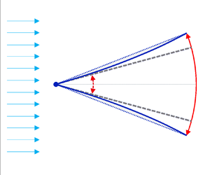
As shown in figure 1, a two-dimensional thin foil with a cord length of c is immersed in an inviscid flow. The pitching motion of the foil is realized by driving its motion at the leading pivot point with a small pitching motion of ${\theta _0}$. The flow has a constant free-stream speed ${U_\infty }$ along the x axis. As a common practice, the origin point is set to the middle point of the foil. As the thin foil pitches along its leading pivot point, the pitching motion will introduce an inertial force caused by the foil and aerodynamical load caused by the surrounding flow to the foil, both of which cause the deformation of the original flat foil. We focus on the small deformation scenario of the foil, where it has sufficient stiffness such that the deformation of the foil is small when compared with its chord.

Figure 1. Schematic of the pitching motion of a thin foil with passive bending deformation. The length scale has been scaled by $c/2$. The pitching angle $\theta $ is the result from the driving pitching angle ${\theta _0}$ and the averaged deformation angle ${\theta _d}$ determined by the deflection of the foil.

To clarify the response of the flexible foil as a result of the driving pitch motion, we use the elastokinetics method to determine the deformation of the foil under the dynamical loading of the inertial force and the aerodynamic fluid force, as has been done in our recent work (Du & Wu 2023). With the deflection of the foil, the averaged deformation angle ${\theta _d}$ of the foil will be introduced. Together with the driving pitch angle at the leading edge and the deformation angle of the foil, the finalized pitching angle of the foil can be determined, as shown in figure 1. As the averaged deformation angle ${\theta _d}$ is sufficiently small, we use a flat foil with the pitching angle $\theta $ to determine the fluid flow, where the camber effect of the foil is ignored in the current study. In the following of this section, we will first introduce the solution to the fluid flow, which gives the pressure loading on the foil analytically. Then, based on the pressure loading and the inertial force on the foil, its deformation will be formulated, from which the averaged deformation angle of the foil can be determined. Together with the deformation angle and the driving pitch motion at the leading point, the pitching motion of the foil will be derived analytically.

2.1. Fluid pressure on the foil

In the pure pitching configuration with small amplitude, as shown in figure 1, the time-harmonic vertical displacement $\mathcal{ H}$ is given by

(2.1)\begin{equation}\mathcal{ H}(x,t) = (x + 1)\,\textrm{tan}\,\theta \cong (1 + x)\theta = \varPhi (1 + x)\,{\textrm{e}^{\textrm{i}2{\rm \pi} t}},\end{equation}

where the length x and $\mathcal{ H}$ have been scaled by half-chord of the foil $c/2$ and the time t has been scaled by the driving flapping period T. The finalized pitching amplitude $\varPhi $ in (2.1) includes the contribution of the driving pitch amplitude and the deformation of the foil, which is the key parameter needed to be determined in this study. Here, $\textrm{i}$ is the imaginary unit and the real part in $\textrm{i}$ should be taken.

In order to determine the pressure distribution on the foil, we resort to the classic solution by Wu (1961). For small amplitude oscillation of the foil in an incompressible inviscid flow, the linear inviscid theory applies and the seminar work of Wu has provided the analytical solution to the flow in detail (Wu 1961). Based on this solution, Moore derived the fluid flow for a flat foil with time-harmonic heaving and pitching kinematics and provided the solution for the pressure distribution on the foil (Moore 2014). We use their solution to obtain the pressure distribution on the pitching foil. Based on the vertical displacement $\mathcal{ H}$ given in (2.1), the fluid flow can be determined by setting ${\beta _0} = 2\varPhi$ and ${\beta _1} = \varPhi $ in (2.5) in Moore's solution (Moore 2014). With the knowledge of the fluid flow, the pressure on the foil, as given in (A7) in Moore's solution (Moore 2014), can be given analytically as

(2.2)\begin{align}p(x,t) = \frac{1}{2}{\rm \pi} \rho {f^2}{c^2}\varPhi \sqrt {1 - {x^2}} \left( {\frac{U}{{1 + x}}\left[ {\textrm{i}(1 - 3{C_k}) - \frac{{U{C_k}}}{{\rm \pi} }} \right] + 4({\rm \pi} - \textrm{i}U) + 2{\rm \pi} x} \right){\textrm{e}^{\textrm{i}2{\rm \pi} t}},\end{align}

where $\rho $ is the density of fluid, $f = 1/T$ is the pitching frequency, $U = 2{U_\infty }/cf$ is the dimensionless free-stream velocity, ${U_\infty }$ is the free-stream velocity in the far field and ${C_k}$ is the well-known Theodorsen function (Theodorsen 1935) given by

(2.3)\begin{equation}{C_k} = \frac{{H_1^{(2)}(k)}}{{\textrm{i}H_0^{(2)}(k) + H_1^{(2)}(k)}} = {F_k} + \textrm{i}{G_k},\end{equation}

where $k = {\rm \pi}fc/{U_\infty } = 2{\rm \pi} /U$ is the reduced frequency, $H_0^{(2)}$ and $H_1^{(2)}$ are the Hankel function of the second kind with orders 0 and 1, respectively. The reduced frequency k can be correlated to the widely used Strouhal number through

(2.4)\begin{equation}St = \frac{\varPhi }{{\rm \pi} }k.\end{equation}

Thus, although we assume the system has a small Strouhal number, the reduced frequency k can be any positive number presuming that the pitching amplitude is small enough. As the pressure distribution given in (2.2) is derived from the incompressible linear inviscid theory, it applies when the Reynolds number is sufficient large such that the viscosity force can be ignored, the oscillation amplitude $\varPhi$ is small such that the disturbance to the flow lies in the linear range and the Strouhal number $St$ of the system is small and the free-stream velocity is much lower than the local sound speed.

2.2. Foil deformation

To determine the foil deformation, the inertial force of the foil will be needed. Thus, the effective displacement of the foil referring to the inertial force will be determined first. As shown in figure 1, the dotted line indicates the chord position of the foil, as has been used to determine the pressure on the foil given in (2.2), which is a straight line $(\kern0.7pt {y_c} = c(1 + x){\theta _d}/2)$ with a rotating angle ${\theta _d}$ compared with the driving pitching position. The finalized foil indicated by the solid line is a curved line, which can be represented by a parabola curve $(\kern0.7pt {y_f} = c{(1 + x)^2}{\theta _d}/4)$ compared with its flat state, if the deformation of the foil is small. Based on the chord line and the parabola curve, the effective displacement of the foil when modelling the inertial force can be approximated by ${y_e} = (\kern0.7pt {y_c} + {y_f})/2 + {y_p}$, where ${y_p} = c(1 + x){\theta _0}/2$ is the displacement introduced by the driving pitching motion ${\theta _0}$ set at the leading edge. As will be shown in this work, without a fluid force, this effective displacement will bring the natural frequency of the foil with the precision of 99.4 % when compared with its exact value. Details of the analytical formulation of the vibration of a cantilever beam can be found in Appendix A. With the effective displacement ${y_e}$, the inertial force on the foil can be given as

(2.5)\begin{equation}{f_i}(x,t) ={-} {m_l}\frac{{{\partial ^2}{y_e}}}{{\partial {t^2}}} ={-} \frac{{{m_l}c}}{2}\left( {\frac{{1 + x}}{2} + \frac{{{{(1 + x)}^2}}}{4}} \right)\frac{{{\partial ^2}{\theta _d}}}{{\partial {t^2}}} - \frac{{{m_l}c(1 + x)}}{2}\frac{{{\partial ^2}{\theta _0}}}{{\partial {t^2}}},\end{equation}

where ${m_l}$ is the line density of the foil.

Based on the pressure load on the foil and the inertial force, the deflection of the foil can be determined by the Euler–Bernoulli beam equation through

(2.6)\begin{equation}\frac{8}{{{c^3}}}B\frac{{{\partial ^4}w}}{{\partial {x^4}}} = {f_i} + p,\end{equation}

where B is the bending stiffness of the foil. The factor $8/{c^3}$ is introduced as the length scale has been scaled by $c/2$. Inserting (2.2) and (2.5) into (2.6), the deflection of the foil w can be solved analytically by including the free boundary condition at the trailing end and the fixed boundary condition at the leading edge. Details of the analytical solution to the deflection are given in Appendix B. From the deflection of the foil, the averaged deformation angle can be given as

(2.7)\begin{equation}{\theta _d} = \int_{ - 1}^1 {\frac{{\partial w}}{{\partial x}}\,\textrm{d}\kern 0.06em x} = \frac{{w(1)}}{2}.\end{equation}

Thus, with the deflection of the foil at the trailing edge $w(1)$, the averaged deformation angle of the foil can be derived as

(2.8) \begin{equation}\begin{aligned} {\theta _d} & ={-} \dfrac{{59{m_l}{c^4}}}{{720B}}\left( {{{\ddot{\theta }}_d} + \dfrac{{66}}{{59}}{{\ddot{\theta }}_0}} \right)\\ & \quad + \dfrac{{{{\rm \pi} ^2}{c^3}}}{{8B}}\left[ {\dfrac{{\rho {f^2}{c^2}}}{4}\dfrac{{25U\left( {\textrm{i}(1 - 3{C_k}) - \dfrac{{U{C_k}}}{{\rm \pi} }} \right)}}{{96}} + \dfrac{{\rho {f^2}{c^2}}}{4}\dfrac{{(109{\rm \pi} - 92\textrm{i}U)}}{{48}}} \right]\varPhi \,{\textrm{e}^{\textrm{i}2{\rm \pi} t}}. \end{aligned}\end{equation}

2.3. Flapping response with flow and foil flexibility coupling

The finalized pitching angle, as shown in figure 1, is given by

(2.9)\begin{equation}\theta = {\theta _0} + {\theta _d}.\end{equation}

By assuming the driving pitch motion ${\theta _0}$ to be ${\varPhi _0}\,{\textrm{e}^{\textrm{i}(2{\rm \pi} t + \vartheta )}}$, with ${\varPhi _0}$ being the driving pitching amplitude and $\vartheta $ is the phase angle between the driving pitching motion and the finalized pitching motion, (2.9) can be reduced to

(2.10) \begin{align}\left. {\begin{array}{*{20}{c}@{}} \begin{array}{l} \dfrac{{{{\rm \pi}^2}{c^3}}}{{8B}}\left[ {\dfrac{{118{m_l}c{f^2}}}{{45}} + \dfrac{{\rho {f^2}{c^2}}}{4}\dfrac{{25U(3{G_k} - U{F_k}/{\rm \pi} )}}{{96}} + \dfrac{{\rho {f^2}{c^2}}}{4}\dfrac{{109{\rm \pi} }}{{48}}} \right]\varPhi \\ \quad + \left( {1 + \dfrac{{7{{\rm \pi}^2}{f^2}{m_l}{c^4}}}{{180B}}} \right){\varPhi _0}\,\textrm{cos}\,\vartheta = \varPhi , \end{array}\\ {\dfrac{{{{\rm \pi}^2}{c^3}}}{{8B}}\left[ {\dfrac{{25(1 - 3{F_k} - U{G_k}/{\rm \pi} )}}{{96}} - \dfrac{{23}}{{12}}} \right]\dfrac{{\rho {f^2}{c^2}U}}{4}\varPhi + \left( {1 + \dfrac{{7{{\rm \pi}^2}{f^2}{m_l}{c^4}}}{{180B}}} \right){\varPhi _0}\,\textrm{sin}\,\vartheta = 0,}\!\!\!\! \end{array}} \right\}\end{align}

from which the finalized pitching amplitude is given by

(2.11)\begin{equation}\varPhi = \frac{{{A_3}}}{{\sqrt {{{(1 - {A_1})}^2} + A_2^2} }}{\varPhi _0}, \end{equation}

and the phase angle is given by

(2.12)\begin{equation}\vartheta = \textrm{atan}\frac{{{A_2}}}{{{A_1} - 1}}.\end{equation}

The dimensionless parameters of ${A_1}$ and ${A_2}$ are given by

(2.13) \begin{equation}\left. {\begin{array}{*{20}{c}} {{A_1} = \dfrac{{3{k^2}}}{{2S}}\left[ {\dfrac{{118}}{{45}}R + \dfrac{{25{\rm \pi} (3{G_k} - 2{F_k}/k)/k + 109{\rm \pi} }}{{192}}} \right],}\\ {{A_2} ={-} \left( {159 + 75{F_k} + \dfrac{{50{G_k}}}{k}} \right)\dfrac{{{\rm \pi} k}}{{128S}},}\\ {{A_3} = 1 + \dfrac{{7R{k^2}}}{{15S}},} \end{array}} \right\}\end{equation}

where $R = {m_l}/\rho c$ is the mass ratio representing the inertia ratio of solid to fluid and $S = 12B/\rho U_\infty ^2{c^3}$ is the dimensionless stiffness of the foil representing the ratio of elastic restoring force to the fluid forces. A nomenclature table for all the symbols is listed in Appendix C. Based on the finalized pitching amplitude and the phase angle, the pitching motion of the foil is finalized, which can be used to determine the deflection of the foil through (B1)–(B7). With the driving pitching motion at the leading edge and the deflection of the foil along its span direction, the snapshots of the flexible foil can be determined. As can be checked, the snapshots show a comparable morphology, as determined by numerical solutions (Floryan & Rowley 2018, 2020). We ignore the snapshots of the foil in this study as we mainly focus on the overall performance of the pitching foil.

From (2.11), we introduce the response parameter $\varUpsilon $ to characterize the response of the flexible foil under driving pitching motion in the fluid flow, which is defined to be

(2.14)\begin{equation}\varUpsilon = \frac{{{{(1 - {A_1})}^2} + A_2^2}}{{A_3^2}} = \frac{{{{\left( {2S - \dfrac{{118}}{{15}}R{k^2} - {a_k}} \right)}^2} + b_k^2}}{{{{\left( {2S + \dfrac{{14}}{{15}}R{k^2}} \right)}^2}}},\end{equation}

where ${a_k}$ and ${b_k}$ are functions of k given by

(2.15)\begin{equation}\left. {\begin{array}{*{20}{c@{}}} {{a_k} = (109{k^2} + 75{G_k}k - 50{F_k})\dfrac{{\rm \pi} }{{64}},}\\ {{b_k} = (159k + 75{F_k}k + 50{G_k})\dfrac{{\rm \pi} }{{64}}.} \end{array}} \right\}\end{equation}

With the parameter of $\varUpsilon $, the finalized pitching amplitude can be given from (2.11) as

(2.16)\begin{equation}\varPhi = \frac{1}{{\sqrt \varUpsilon }}{\varPhi _0}.\end{equation}

Therefore, the complex interaction between the flexible foil and the surrounding fluid flow will be determined by the value of $\varUpsilon $, which is a function of the mass ratio R, the dimensionless stiffness S and the reduced frequency k. While ${a_k}$ and ${b_k}$ surely influence the response of the pitching foil, we show their value as a function of the reduced frequency k in figure 2. It shows that, when k reduces from 1 to zero, ${a_k}$ and ${b_k}$ will decrease from their positive values to the negative ones and finally approach the fixed values determined by ${F_k}$ and ${G_k}$, respectively. On the other side, if k is larger than 1, ${a_k}$ and ${b_k}$ will increase with increasing k and their values will scale with ${k^2}$ and k, respectively, if k is large enough, say larger than 10.

Figure 2. Values of ${a_k}$ and ${b_k}$ as a function of the reduced frequency k in the value ranges of (a) 0.001 to 1 and (b) 1 to 1000.

The finalized pitching amplitude given in (2.16) shows a rather simple form compared with the reported analytical solutions. To check its accuracy, we first check the natural frequency of the system without a fluid force. Under this condition, ${a_k}$ and ${b_k}$ vanish and $\varUpsilon = {(2S - 118R{k^2}/15)^2}/{(2S + 14R{k^2}/15)^2}$. Therefore, resonation happens if $\varUpsilon = 0$, which gives the reduced frequency ${k_0}$ as

(2.17)\begin{equation}{k_0} = \sqrt {\frac{{15S}}{{59R}}} .\end{equation}

This gives ${k_0} \approx 0.5042\sqrt {S/R} $, which compares well with ${k_0} \approx 0.5075\sqrt {S/R} $ from the exact result for the first resonant frequency of a cantilever beam (Rao 2011) and is more precise than the value of ${k_0} \approx 0.497\sqrt {S/R} $ obtained from a quartic-order approximation to the beam deformation provided by Fernandez-Feria & Alaminos-Quesada (2021).

On the other hand, if the fluid–structure interaction is included, the resonance frequency will be determined by the minimum value of $\varUpsilon $ under given S and R. Although a numerical procedure is needed to determine the resonation frequency ${k_r}$ in general, we can propose an approximation analytical relation between S, R and the resonant frequency ${k_r}$. This is realized by observing that, for given k and R, the minimum value for $\varUpsilon $ is reached if

(2.18)\begin{equation}\frac{{\partial \varUpsilon }}{{\partial S}} = \frac{4}{{{{\left( {2S + \dfrac{{14}}{{15}}R{k^2}} \right)}^3}}}\left[ {\left( {2S - \frac{{118}}{{15}}R{k^2} - {a_k}} \right)\left( {\frac{{44}}{5}R{k^2} + {a_k}} \right) - b_k^2} \right] = 0,\end{equation}

from which the analytical relation between S, R and the resonation frequency ${k_r}$ can be given as

(2.19)\begin{equation}{S_r} = \frac{1}{2}\left( {\frac{{118}}{{15}}Rk_r^2 + {a_k} + \frac{{b_k^2}}{{\dfrac{{44}}{5}Rk_r^2 + {a_k}}}} \right).\end{equation}

It can be easily checked from (2.19) that, if R is large enough, the resonation frequency ${k_r}$ will reduce to (2.17), that is the resonation is regulated by the elasticity of the foil. If R is much smaller than unity, its effect may be ignored and the resonance will be determined by

(2.20)\begin{equation}{S_r} = \frac{1}{2}\left( {{a_k} + \frac{{b_k^2}}{{{a_k}}}} \right).\end{equation}

2.4. Model validation

For the dimensionless stiffness of $S = 10$, we compare the resonance frequency ${k_r}$ as a function of R between our theory and that from previous theories. The result shown in figure 3(a) clearly demonstrates the accuracy of our theory in capturing the resonance frequency of this flow–structure system. While the numerical result determined by Floryan & Rowley (2018) (F & R) is based on a more general theory (Floryan & Rowley 2018), which can be treated as the exact solution to the problem, our numerical solution seems to match as well as that from the solution obtained by Fernandez-Feria & Alaminos-Quesada (2021) (F & A) (Fernandez-Feria & Alaminos-Quesada 2021) when the mass ratio R is small ($R < 0.1$) and matches better than F & A when R is large ($R > 1$). Furthermore, among all these theoretical models, the analytical relation given in (2.19) shows a comparable match to the result of F & R (Floryan & Rowley 2018), thus demonstrating the applicability of our analytical solution to the flow–structure interaction problem.

Figure 3. The resonance frequency ${k_r}$ as a function of (a) mass ratio R for dimensionless stiffness of $S = 10$ and (b) dimensionless stiffness S for mass ratio of $R = 0.01$. The results from F & A (Fernandez-Feria & Alaminos-Quesada 2021) and F & R (Floryan & Rowley 2018) are included for comparison, where the result of F & R can be treated as exact. The star in (a) corresponds to (2.20).

For a mass ratio of $R = 0.01$, we compare the resonance frequency ${k_r}$ as a function of S between our theory and that from the previous theory of F & R (Floryan & Rowley 2018). The result shown in figure 3(b) shows that, when the dimensionless stiffness S is large, the numerical solution from (2.14) can always provide a comparable resonance frequency ${k_r}$ to that from F & R (Floryan & Rowley 2018). However, when the dimensionless stiffness S is small, the resonance frequency ${k_r}$ determined from our theory is different from the results given by F & R (Floryan & Rowley 2018). This is caused by the fact that our theory is based on Euler–Bernoulli beam theory, which cannot recover the flutter type resonance branch emerging when the dimensionless stiffness S is sufficient small ($S \le 0.1$). Figure 3(b) also shows that the analytical relation given in (2.19) can provide a meaningful value when the dimensionless stiffness S is larger than a typical value of 10 and the reduced frequency k is larger than 1. This is because the analytical relation given in (2.19) is derived by assuming that k and R are both fixed, which means that the minimization of $\varUpsilon $ over S can only bring the local ones to $\varUpsilon $. For given mass ratio R of the pitching foil, these local minimum values of $\varUpsilon $ are coincidence with the global ones only when the dimensionless stiffness S and the reduced frequency k are larger than their corresponding certain critical values.

To further validate our theoretical model, we make a direct comparison on the response parameter $\varUpsilon $ between our theoretical model and direct simulation with data extracted from Peng et al. (2022). As shown in figure 4, the match is good between our theoretical model and the simulation for broad ranges of dimensionless stiffness and reduced frequency. Both model and simulation show that, when the dimensionless stiffness increases, the response parameter $\varUpsilon $ will decrease firstly and reach a minimum value and then approach to the constant of 1. The minimum value for $\varUpsilon $ corresponds to the resonance condition, whereas $\varUpsilon = 1$ corresponds to an equal pitching amplitude between the finalized pitching motion and the driving one. For the resonance condition, our model can nicely recover the critical dimensionless stiffness for resonance, as shown by the thin vertical lines. For the equal pitching amplitude condition ($\varUpsilon = 1$), both theoretical model and simulation show that there is a critical dimensionless stiffness satisfying this condition and this critical dimensionless stiffness increases as the reduced frequency increases. Although the exact value varies a bit between the theoretical model and simulation, our theoretical model can recover the trends for the critical dimensionless stiffness as a function of the reduced frequency.

Figure 4. The response parameter $\varUpsilon $ as a function of the dimensionless stiffness while under different reduced frequencies k from 1.257 to 3.770 shown by lines and symbols with different colours. The scatters are the results from direct simulation extracted from Peng et al. (2022), with the driving pitching amplitude of 0.1 and mass ratio of 1. The dashed line is corresponding to $\varUpsilon = 1$ and the dotted line is corresponding to $\varUpsilon = 0.3$. The vertical thin lines correspond to the resonance condition determined from simulation. The inset shows the trailing amplitude normalized by the span of the foil, with the reduced frequency k of 3.142.

When driving at resonance condition, our model fails to give the accurate response parameter as that from simulation provided by Peng et al. (2022). This is because the driving pitching amplitude used by Peng et al. is 0.1, which makes the finalized pitching amplitude obviously larger than the ones that the linear inviscid theory holds. As shown in the inset of figure 4, for the corresponding trailing amplitude of the flexible foil, our theoretical model matches quantitatively with the simulations both for the resonance stiffness and the corresponding trailing amplitude when the dimensionless stiffness is away from the resonance value. Near the resonance condition, the finalized pitching amplitude will be as large as 0.4, which is obviously beyond the regime in which linear inviscid theory can be utilized. In fact, we have checked that, when the driving pitching amplitude is small, such that the linear inviscid theory still holds, our theory can reasonably recover the resonance pitching amplitude.

Overall, based on the comparison between our theoretical model and these previous models (Floryan & Rowley 2018; Fernandez-Feria & Alaminos-Quesada 2021) and direct simulations (Peng et al. 2022), the response parameter $\varUpsilon $ coined in this work could nicely forecast the response of the flexible foil when pitching at the leading edge, demonstrating the suitability of using it to uncover the physics of the flow–structure interaction system.

3. Results and discussions

In § 2, we have presented the analytical formulation for the response of the flexible foil as a result of the driving pitch motion at the leading edge. Based on this formulation, this section presents the results of the kinematics and the propulsion performance of the pitching flexible foil. While the response of the pitching foil is solely determined by the mass ratio R, the dimensionless stiffness S and the reduced frequency k, in this section, a broad parameter ranges including $S \in [0.1,1000]$, $k \in [0.1,100]$ and $R \in [0.01,10]$ will be used to determine the response of the pitching foil. Based on these parameter ranges, the pitching amplitude and the phase angle will be determined first and then the thrust and propulsive efficiency will be presented. Here, a lower mass ratio of $R = 0.01$ corresponds to underwater swimmers and higher ones of $R \ge 1$ correspond to fliers.

3.1. Pitching amplitude

The responded pitching amplitude given in (2.16) shows a linear relation with the driving pitch amplitude, with the coefficient determined by $\varUpsilon $, which is given by (2.14). While the resonance condition of the foil has been clarified in § 2 as well as in these previous reports, here, we mainly focus on the critical condition that defines the situation when the flexibility of the foil enlarges the pitching amplitude. Based on (2.14), this condition can be readily given by $\varUpsilon < {\varUpsilon _e} = 1$, which gives

(3.1)\begin{equation}{S_e} = \frac{1}{4}\left[ {\left( {\frac{{118}}{{15}}R{k^2} + {a_k}} \right) + \frac{{b_k^2}}{{\left( {\dfrac{{44}}{5}R{k^2} + {a_k}} \right)}}} \right].\end{equation}

Comparing (2.19) and (3.1), it shows that, for a given reduced frequency k and mass ratio R, the dimensionless stiffness S for resonance is twice as the critical one where the flexibility of the foil does not change the pitching amplitude. This relation applies when (2.19) can capture the resonance condition of the foil. From (3.1), we can determine the critical reduced frequency k in principle as there is no other unknown parameter if S and R are given.

The analytical expression of (3.1) implies there is a minimum value for ${S_e}$, indicated as ${S_{em}}$, below which there is no solution for the reduced frequency k. To check this statement, we show the map of ${S_e}$ as a function of R and k in figure 5. It shows that, for a given mass ratio $R$ in the range 0.01–10, there is a global minimum for the positive value of ${S_e}$, where the value for k is indicated as the solid line. Figure 5 also shows that, although the value for R spans four orders, the critical value for k just spans one order, indicating the value of the critical reduced frequency k is insensitive to the mass ratio R. The existence of the value ${S_{em}}$ indicates that the foil should have sufficient bending stiffness such that its pitching amplitude can be enlarged as a result of deformation, although infinite bending stiffness will never change the pitching amplitude either.

Figure 5. The map of ${S_e}$ as a function of the mass ratio R and the reduced frequency k. The solid line is corresponding to ${S_{em}}$ by numerical determining the minimum value from (3.1). The dotted line is corresponding to (3.3). The region for the value of ${S_e}$ larger than 15 is whited out and that smaller than zero is greyed out.

As the minimum value for ${S_e}$, or ${S_{em}}$, determines whether the flexibility of the foil can enlarge the pitching amplitude, we propose an approximated analytical solution to ${S_{em}}$ here. Based on (3.1), if treating $44R{k^2}/5 + {a_k}$ as the unknown parameter that needs to be determined, then it has solution only when

(3.2)\begin{equation}\Delta = {\left( {4{S_{em}} + \frac{{14}}{{15}}R{k^2}} \right)^2} - 4b_k^2 \ge 0.\end{equation}

This readily gives the value of ${S_{em}}$, below which there is no solution to (3.1); that is, if $S < {S_{em}}$ the pitching amplitude can never surpass its rigid counterpart. Here, ${S_{em}}$ can be given by

(3.3)\begin{equation}2{S_{em}} + \frac{7}{{15}}R{k^2} = {b_k} = \frac{{44}}{5}Rk_m^2 + {a_k},\end{equation}

where ${k_m}$ is the corresponding reduced frequency. Equation (3.3) shows how to determine the lower value of ${S_{em}}$, which is realized by determining ${k_m}$ through the second equality if the mass ratio R is specified. While (3.2) indicates the absolute treatment should be put on ${b_k}$, implying there may be two solutions to k, we can show that, for R in the range between 0.01 and 10, only the solution that guarantees a positive ${b_k}$ is legitimate, as has been given in (3.3). To do so, we show the relation of (3.3) as the dotted line in figure 5. For a given value of R lying in the range of 0.01 and 10, figure 5 shows that the value for ${k_m}$ that satisfies (3.3) lies in the range between 0.1 and 1. Based on the value range of ${k_m}$ and checking the value of ${b_k}$ from figure 2, it clearly shows that ${b_k}$ is always positive. This justifies the suitability of choosing the positive value for ${b_k}$ in (3.3) when determining the critical dimensionless stiffness ${S_{em}}$.

To check the suitability of (3.3) in determining the minimum value for ${S_{em}}$, we make a comparison between the results from (3.1) and (3.3), which have been shown by the solid line and dotted line in figure 5. The lines from figure 5 shows that the analytical relation given in (3.3) can provide a pretty good solution to ${S_{em}}$ when compared with that of the numerical results from (3.1) if the mass ratio R is large, say larger than 1. Under this condition, k approaches 0.1 and ${b_k}$ approaches zero slowly. When R is small, there is a notable discrepancy between them, indicating the analytical relation of (3.3) failed to provide the global minimum value for ${S_e}$. This is because (3.3) implies the global minimum for ${S_e}$ happens when ${b_k} = 44Rk_m^2/4 + {a_k}$ has been satisfied. While this is true only when ${b_k}$ is constant over k, this surely breaks down as ${b_k}$ is in principle a function of k. However, the weak dependence of ${b_k}$ as a function of k when k approaches zero guarantees that the analytical relation proposed in (3.3) can provide a reliable value for ${S_{em}}$, which happens to be the condition when the mass ratio R is large and the corresponding value of ${k_m}$ is sufficiently small.

With the information for the minimum value of ${S_e}$, we move to determine the analytical relation among R, S and k, which defines whether the flexibility of the foil can enlarge the pitching amplitude. If (3.2) can be satisfied, the solution to $44R{k^2}/5 + {a_k}$ can be given from (3.1) through

(3.4)\begin{equation}\frac{{44}}{5}R{k^2} + {a_k} = \left( {2S + \frac{7}{{15}}R{k^2}} \right) \pm \sqrt {{{\left( {2S + \frac{7}{{15}}R{k^2}} \right)}^2} - b_k^2} .\end{equation}

As with the intermediate functions of ${a_k}$ and ${b_k}$, these is no simple analytical solution to k in general. Here, we can formulate asymptotic relations among R, S and k as follows. While (3.1) has been used to derive the lower boundary for the dimensionless stiffness, here we consider the condition when the dimensionless stiffness approaches a large value. Under this condition, we will demonstrate that the condition of $4{S^2} \gg b_k^2$ can be always satisfied. Based on this relation, two asymptotic relations can be obtained from (3.4). The first one determines the lower solution for the reduced frequency ${k_l}$ as

(3.5)\begin{equation}\frac{{44}}{5}Rk_l^2 + {a_k} = 0.\end{equation}

This relation is rather simple, indicating that there is a critical reduced frequency, denoted by ${k_l}$, which is solely determined by R if the value of S is large; that is, ${k_l}\sim f(R)$. It can be easily checked that this critical reduced frequency ${k_l}$ is the lower boundary for the reduced frequency, below which the pitching amplitude of the flexible foil will be smaller than the rigid counterpart. The second asymptotic relation determines the upper boundary for the reduced frequency, denoted by ${k_u}$, as

(3.6)\begin{equation}\frac{{118}}{{15}}Rk_u^2 + {a_k} = 4S.\end{equation}

Based on the definition for ${a_k}$ given by (2.15), the asymptotic solution for the reduced frequency ${k_u}$ can be given as

(3.7)\begin{equation}{k_u} \cong \frac{2}{{\sqrt {\dfrac{{118}}{{15}}R + \dfrac{{109{\rm \pi} }}{{64}}} }}\sqrt S .\end{equation}

From (3.7), it shows that the solution for ${k_u}$ satisfies $S\sim k_u^2$ if S is sufficiently large. As ${k_u}$ is the upper boundary for the reduce frequency k, the condition of $4{S^2} \gg b_k^2$ can be easily justified if we note that ${b_k}\sim k$, as the results from figure 2(b) show.

With these analytical relations for the equal pitching amplitude condition, whether the foil with flexibility has a larger pitching amplitude can be easily checked. Firstly, we need to check that the dimensionless stiffness S is larger than the lower boundary determined by (3.3) analytically or the more accurate one of the minimum from (3.1) numerically. If this can be satisfied, we need to determine the lower and upper boundaries for the reduced frequency through (3.5) and (3.7), respectively. If the reduced frequency from the working condition lies between them, the foil will have a larger pitching amplitude than the driving one. Otherwise, the pitching amplitude of the foil will decrease as a result of deformation.

For mass ratios of 0.01 and 1, figure 6 show the pitching amplitudes as a function of dimensionless stiffness S and reduced frequency k, together with the resonance condition defined from (2.14) and the equal pitching amplitude condition of $\varUpsilon = 1$ defined from (3.1). In order to justify the accuracy of the physical model proposed in this study, we also included these previously reported results in figure 6. For a mass ratio of 0.01, we make a comparison between our theoretical model with the result from F & R (Floryan & Rowley 2018). As shown in figure 6(a), the reduced frequency for resonance matches well between our theory and that from F & R when the dimensionless stiffness S is relatively large. Under this condition, the corresponding resonance frequency ${k_r}$ scales with S with a power of 1/2, as (2.19) implies. The match becomes worse if the dimensionless stiffness S is small, under which ${k_r}$ is smaller from our theory when compared with F & R. Besides the resonance condition, the relation between the reduced frequency k and the dimensionless stiffness ${S_e}$ for $\varUpsilon = 1$ is consistent between our theory of (3.1) and the results from F & R. For the equal pitching amplitude condition, although our theory will shift the reduced frequency down a bit, both theories give that there is a critical stiffness ${S_{em}}$ below which the pitching amplitude will decrease no matter the reduced frequency k. All these results indicate that our theory can provide a meaningful method to evaluate the flexibility effect on the pitching foil, if noting that our theory has the simple closed-form expressions.

Figure 6. Pitching amplitudes as a function of dimensionless stiffness S and reduced frequency k for given mass ratio of (a) $R = 0.01$ and (b) $R = 1$. The solid red lines correspond to the natural frequency obtained from minimization of (2.14) numerically. The solid black lines correspond to the solution given by (3.1), where the dashed black lines correspond to (3.3), (3.5) and (3.7), respectively. The dashed red line and the dotted line in (a) correspond to the result from F & R (Floryan & Rowley 2018). The cycle scatters in (b) correspond to the results from Peng et al. (2022).

In figure 6(b), we include the simulated results from Peng et al. (2022) as shown by these scattered symbols. The comparison between our theory and the simulated ones shows that the theory proposed in this study can nicely capture the effect of the flexibility of the foil on the pitching amplitude, although a certain discrepancy does exist between them if the exact pitching amplitude is concerned. The discrepancy is introduced as the pitching amplitude of the foil is well above 0.1 and even reaches up to 0.2 in their simulations (Peng et al. 2022). With such large pitching amplitudes, the linear potential flow theory used in this study surely breaks down. Although, with this limitation, the predictive ability of the theoretical model in forecasting the pitching amplitude for a flexible foil is still evident.

Next, we justify the analytical relations for $\varUpsilon = 1$ formulated in this study. For a low mass ratio of $R = 0.01$ and a relatively high mass ratio of $R = 1$, figure 6(a,b) shows that the flexibility of the foil may increase or decrease the pitching amplitude, which is determined by the combination of the dimensionless stiffness S and the reduced frequency k if the mass ratio R is given. When the reduced frequency is large ($k > 2$), figure 6(a,b) shows that this critical stiffness ${S_{em}}$ for equal pitching amplitude is half of the stiffness at which resonance happens. To obtain a larger pitching amplitude, the dimensionless stiffness S should be larger than 6.92 if the mass ratio is 0.01, under which the reduced frequency is approximately 1.14. For a mass ratio of 1, the minimum dimensionless stiffness S is 2.88 and the corresponding reduced frequency is 0.57. These critical values for S are determined from the numerical minimization of (3.1). If the analytical relation of (3.3) is used to determine the critical values, for R to be 0.01 and 1, the dimensionless stiffness turns out to be 9.26 and 3.73, with the corresponding reduced frequency being 1.93 and 0.82, respectively, as indicated by the stars in these panels. The comparison of the minimum stiffness between the numerical solution and that from the analytical relation shows that the analytical relation given by (3.3) is more suitable for the larger mass ratio condition. Although with a certain discrepancy between the analytical results compared with the numerical solutions, the analytical relation of (3.3) can provide a meaningful value for the minimum dimensionless stiffness ${S_{em}}$.

If the dimensionless stiffness is larger than ${S_{em}}$, the pitching amplitude can be larger than the rigid counterpart only when the reduced frequency k is located between the lower boundary determined by ${k_l}$ and the upper boundary determined by ${k_u}$, as figure 6 shows. Figure 6(a,b) shows that the lower boundary of ${k_l}$ is constant over S if S is sufficiently large, which is solely determined by R, as the horizontal dashed lines in these figures show. For R to be 0.01 and 1, ${k_l}$ is 0.57 and 0.35, respectively, both of which can be readily determined from (3.5). As for the upper boundary of ${k_u}$, the tilted dashed lines determined from (3.7) match nicely with the upper boundary of the reduced frequency determined numerically from (3.1). Both figures show that ${k_u}$ scales with the dimensionless stiffness S with a power of 1/2, as (3.7) gives. These consistencies between the numerical solutions and the analytical relations demonstrate the suitability of these analytical relations in forecasting the equal pitching amplitude condition as a result of foil flexibility.

In a recent computation work, Peng et al. proposed that the finalized pitching amplitude can collapse into a single line if the driving frequency is normalized by the resonance frequency ${k_r}$ (Peng et al. 2022). To check this statement, for dimensionless stiffness S ranging from 0.1 to 1000 and mass ratios R of 0.01, 1 and 10, we determine the pitching amplitude as a function of the ratio between the reduced frequency and the resonance frequency. The result is shown in figure 7, which shows that the dimensionless stiffness S will influence the collapse of those curves whereas the mass ratio R will influence the peak value of the normalized pitching amplitude. The collapse of these curves holds only when the dimensionless stiffness S is sufficient large, say larger than 10 in this pitching motion. This is consistent with the parameter range presented by Peng et al. (2022), where most of the dimensionless stiffness S is well above 10, thus justifying their method of collapsing the pitching amplitude by the normalized frequency. Noting that the dimensionless stiffness $S = 12K$, where K is the scaled bending stiffness defined by Peng et al. (2022). If the dimensionless stiffness S is smaller than 10, the normalized pitching amplitude will shift to a lower value when compared with the higher dimensionless stiffness S condition, indicating the collapse of the pitching amplitude curves fails.

Figure 7. Pitching amplitude as a function of frequency ratio for dimensionless stiffness S ranging from 0.1 to 1000 as shown in lines with different colours. The solid lines, dashed lines and dotted lines correspond to mass ratios R of 10, 1 and 0.01, respectively.

For the effect of the mass ratio R, figure 7 shows that it acts like the damping parameter for a damped resonant system, where the peaks for the pitching amplitude are corresponding to damped resonances, with damping scaling inversely with the mass ratio R, as has been observed by Zhang, Zhou & Luo (2017). For a high mass ratio R ($R \ge 1$), there is a sharp peak for the normalized pitching amplitude, which is smoothed out if the mass ratio is small ($R = 0.01$), indicating strong damping exists under this condition. However, one may suspect their similarity if making a comparison on the dissipative properties between this flow–structure system and the damped resonant system. This is because, while the damped resonant system is clearly a dissipative system, where the input power has been fully dissipated by the damping of the system, this flow–structure system belongs to the non-dissipative system as the flow is inviscid. To reconcile this difference, we can isolate the foil from the flow–structure system, where the input power used to drive its pitching motion is readily dissipated by, or transferred to, the flow, which increases the kinetic energy of the flow steadily. Thus, with this analogy, the mass ratio R will signify the energy transfer ability from the foil to the flow; a lower value of R contributes to higher energy transfer ability and vice versa.

To further evaluate the maximum pitching amplitude for flexible foils, we determine the map of the pitching amplitude at resonance as a function of the dimensionless stiffness S and the mass ratio R in figure 8(a), together with the corresponding resonance frequency ${k_r}$ shown in figure 8(b). For the parameter ranges investigated in this study, figure 8(a) shows the peak amplitude is mainly regulated by the dimensionless stiffness S, larger stiffness introduces larger peak pitching amplitude. For given mass ratio R, there is a critical S, below which the peak pitching amplitude is smaller than the driving pitching amplitude. While the mass ratio R spans in three orders, the critical S increases slowly from 0.60 to 6.53, demonstrating S is the main contribution to the peak pitching amplitude. We remark that caution needs to be employed when using figure 8(a) to evaluate the maximum pitching amplitude obtainable, especially concerning the up to 2 orders of amplification to the driving amplitude. Under these conditions, the pitching angle will become so large that flow separation and other high-order effects are highly possible, making the linear potential flow theory used in this study fail. The map for the resonance frequency ${k_r}$ shown in figure 8(b) indicates that the resonance frequency is mainly regulated by the dimensionless stiffness S, although the effect of R is evident if S is small. For the critical condition that the peak pitching amplitude is the same as the driving one, the resonance frequency also lies in a narrow range between 0.19 and 1.07, which changes slowly with the mass ratio R in a non-monotonic way.

Figure 8. Map of (a) the pitching amplitude at resonance ${\varPhi _r}$ and (b) the resonance frequency ${k_r}$ as a function of dimensionless stiffness S and mass ratio R. The solid line in (a) corresponds to the condition that the peak pitching amplitude is the same as the driving pitching amplitude.

3.2. Phase angle

For the phase angle given in (2.12), it can be represented through ${a_k}$ and ${b_k}$ as

(3.8)\begin{equation}\vartheta = \textrm{atan}\frac{{{b_k}}}{{2S - 118R{k^2}/15 - {a_k}}}.\end{equation}

Thus, whether the phase angle is larger or smaller than zero is determined by the following two conditions. The first one is ${b_k} = 0$, from which the reduced frequency k is determined to be 0.0092, as figure 2 shows. When k is larger than 0.0092, the value of ${b_k}$ is positive, and vice versa. The second one is

(3.9)\begin{equation}{S_p} = \frac{{59R{k^2}}}{{15}} + \frac{1}{2}{a_k}.\end{equation}

We show that the critical condition given in (3.9) controls the sign of the phase angle uniquely. This is because the value of k in this study is mainly located in the range of 0.1–100, which guarantees that ${b_k}$ is always positive. In fact, (3.9) not only determines the sign of the phase angle, but also determines the quadrature condition between the driving pitching motion and finalized pitching motion, where the phase angle is ${\pm} {\rm \pi}/2$.

It shows from (3.9) that, for a given mass ratio R, the reduced frequency k will separate the dimensionless stiffness ${S_p}$ into two regions. These two regions have been shown in figure 9. The first region is the grey coloured region, as shown in figure 9 in the lower part. In this region, the value of ${S_p}$ is negative all the time. This indicates the value of $2S - 118R{k^2}/15 - {a_k}$ will be positive for any dimensionless stiffness S, meaning the phase angle is positive over the dimensionless stiffness of the foil. The second region is the upper part shown in figure 9, where the value of ${S_p}$ is positive. Under this condition, the value of $2S - 118R{k^2}/15 - {a_k}$ will be positive when the dimensionless stiffness S is larger than ${S_p}$, which brings a positive value to the phase angle. On the other side, the phase angle is negative. If the critical condition of $S = {S_p}$ can be satisfied, the phase angle will be ${\pm} {\rm \pi}/2$, indicating the driving pitching motion and the finalized pitching motion are quadrature.

Figure 9. The value of ${S_p}$ as a function of mass ratio R and reduced frequency k. The grey region defined by the line of ${S_p} = 0$ corresponds to the positive phase angle no matter the dimensionless stiffness of the foil.

When elucidating the connections between the pitching amplitude and the phase angle, it can be easily checked from (3.9) for ${S_p}$ and (3.3) for ${S_{em}}$ that the critical dimensionless stiffness for these two conditions is the same. While the connection between the phase angle and the resonance of the pitching foil is less obvious, we observe that, when the reduced frequency k is large, the condition for resonance is the same as the condition when the quadrature happens to the pitching foil, where the phase angle equals to ${\pm} {\rm \pi}/2$. This is because, when k is large, both the resonance deduced stiffness from (2.19) and the phase angle of ${\pm} {\rm \pi}/2$ deduced stiffness from (3.9) scale the same as $(118R/15 + 109{\rm \pi} /128){k^2}$. To check this statement, we show the phase angle of the foil as a function of S and k both for $R = 0.01$ and $R = 1$ in figure 10. Figure 10(a,b) shows that, when the reduced frequency k is large, the match is good between the resonance derived dimensionless stiffness ${S_r}$ and the phase angle of ${\pm} {\rm \pi}/2$ derived dimensionless stiffness ${S_p}$. When the reduced frequency k is small, there is certain discrepancy between ${S_r}$ and ${S_p}$, and this discrepancy is more evident when the mass ratio is small. This is because (3.9) can provide the correct resonance dimensionless stiffness ${S_r}$ only when R and k are sufficiently large. Otherwise, it will bring a certain discrepancy to ${S_r}$, as has been shown in figure 3(b). Besides this discrepancy, figure 10(a,b) shows that, when the stiffness S is larger than ${S_p}$, the phase angle will be positive, and vice versa.

Figure 10. Phase angle $\vartheta $ as a function of dimensionless stiffness S and reduced frequency k for different mass ratios of (a) $R = 0.01$ and (b) $R = 1$. The dashed lines correspond to the natural frequency given by (2.14), as indicated by ${S_r}$.

3.3. Thrust generation

The forward thrust of the pitching foil contains two parts; namely, the leading-edge suction resulting from the flow singularity at the leading-edge point and the contribution from the pressure difference on the foil. Following Moore's solution (Moore 2014), the leading-edge suction induced thrust ${T_s}$ can be calculated by contour integration as

(3.10)\begin{equation}{T_s}(t) = {\textstyle{1 \over 4}}{\rm \pi} \rho {c^3}{f^2}{\varPhi ^2}[{(3{\rm \pi} {G_k} - U{F_k})^2}\,\textrm{co}{\textrm{s}^2}\,2{\rm \pi} t + {({\rm \pi} - 3{\rm \pi} {F_k} - U{G_k})^2}\,\textrm{si}{\textrm{n}^2}\,2{\rm \pi} t].\end{equation}

The pressure induced thrust ${T_p}$ is given by

(3.11)\begin{equation}{T_p}(t) = {\textstyle{1 \over 4}}{\rm \pi} \rho {c^3}{f^2}{\varPhi ^2}(3{\rm \pi} U{G_k} - {U^2}{F_k} + 2{{\rm \pi} ^2})\,\textrm{co}{\textrm{s}^2}\,2{\rm \pi} t.\end{equation}

Thus, the time averaged forward thrust ${T_m}$ and the fluctuation amplitude ${T_a}$ of the forward thrust of the pitching foil can be determined as

(3.12) \begin{equation}\left. {\begin{array}{*{20}{c@{}}} {{T_m} = \dfrac{1}{8}{{\rm \pi}^3}\rho {c^3}{f^2}{\varPhi^2}\left[ {{{\left( {3{G_k} - \dfrac{2}{k}{F_k}} \right)}^2} + 2\left( {\dfrac{3}{k}{G_k} - \dfrac{2}{{{k^2}}}{F_k} + 1} \right) + {{\left( {1 - 3{F_k} - \dfrac{2}{k}{G_k}} \right)}^2}} \right],}\\ {{T_a} = \dfrac{1}{8}{{\rm \pi}^3}\rho {c^3}{f^2}{\varPhi^2}\left[ {{{\left( {3{G_k} - \dfrac{2}{k}{F_k}} \right)}^2} + 2\left( {\dfrac{3}{k}{G_k} - \dfrac{2}{{{k^2}}}{F_k} + 1} \right) - {{\left( {1 - 3{F_k} - \dfrac{2}{k}{G_k}} \right)}^2}} \right].} \end{array}} \right\}\end{equation}

After being normalized by the force $\rho U_\infty ^2c/2$, the coefficient of the mean thrust ${C_{Tm}}$ and its fluctuation amplitude ${C_{Ta}}$ can be given as

(3.13)\begin{equation}\left. {\begin{array}{*{20}{c@{}}} {{C_{Tm}} = \dfrac{1}{\varUpsilon }{C_{Tm0}},}\\ {{C_{Ta}} = \dfrac{1}{\varUpsilon }{C_{Ta0}},} \end{array}} \right\}\end{equation}

where the relation of (2.16) has been used. Here, ${C_{Tm0}}$ and ${C_{Ta0}}$ are the coefficient of the mean thrust and its fluctuation amplitude of the rigid foil counterpart given by

(3.14)\begin{equation}\left. {\begin{array}{*{20}{c@{}}} {{C_{Tm0}} = \dfrac{{{\rm \pi} \varPhi_0^2}}{4}[{{(3k{G_k} - 2{F_k})}^2} + 2(3k{G_k} - 2{F_k} + {k^2}) + {{(k - 3k{F_k} - 2{G_k})}^2}],}\\ {{C_{Ta0}} = \dfrac{{{\rm \pi} \varPhi_0^2}}{4}[{{(3k{G_k} - 2{F_k})}^2} + 2(3k{G_k} - 2{F_k} + {k^2}) - {{(k - 3k{F_k} - 2{G_k})}^2}].} \end{array}} \right\}\end{equation}

Based on (3.13), the effect of the flexibility of the foil on the thrust generation is evident, which is solely determined by the response parameter $\varUpsilon $ that was introduced in (2.14). While the value of $\varUpsilon $, which determines the normalized pitching amplitude, as a function of the dimensionless stiffness S, the mass ratio R and the reduced frequency k has been elucidated in detailed in § 3.1, here, we make a short summary for the thrust coefficients of the rigid foil. As shown in figure 11, the mean thrust ${C_{Tm0}}$ will increase monotonically with the reduced frequency k and a scaling between them can be easily obtained from (3.14) as ${C_{Tm0}}\sim 9{\rm \pi} \varPhi _0^2{k^2}/16$, if we note that ${F_k}\sim 0.5$ and ${G_k}\sim 0$ when $k \to + \infty $. When the reduced frequency k reduces to 0.635, the mean thrust changes from positive to negative, meaning the drag to thrust (DTT) transition happens when $k = 0.635$. For the ratio of the fluctuation amplitude to the mean thrust ${C_{Ta0}}/{C_{Tm0}}$, figure 11 shows that it increases with the reduced frequency k and will approach a constant when the reduced frequency k is sufficiently large; say larger than 3. The constant is 7/9, meaning the foil will always encounter forward thrust when pitching in fluid.

Figure 11. Coefficient of the mean thrust ${C_{Tm0}}$ and the ratio between the fluctuation thrust amplitude and the mean thrust ${C_{Ta0}}/{C_{Tm0}}$ for a rigid foil as a function of reduced frequency k. The amplitude of the driving pitching angle is set to be 1.

For foil pitching in a ‘real’ fluid, the viscosity of the fluid will inevitably introduce offset drag to the foil, which reduces its forward thrust. While some of the theoretical models included a constant offset drag coefficient to the foil (Floryan et al. 2017; Fernandez-Feria & Alaminos-Quesada 2021), here, we introduce a projected frontal area related offset drag coefficient to the foil, which resembles a bluff body moving in fluid (Floryan, Van Buren & Smits 2018; Van Buren, Floryan & Smits 2019). So, the offset drag coefficient ${C_d}$ can be given as

(3.15)\begin{equation}{C_d} = \xi \varPhi = \frac{1}{{\sqrt \varUpsilon }}\xi {\varPhi _0},\end{equation}

where $\xi $ is constant. For a rigid foil, the offset drag coefficient is given by ${C_{d0}} = \xi {\varPhi _0}$. Based on their experimental investigation, Van Buren et al. fitted a value of 0.48 for the constant $\xi $ (Van Buren et al. 2019). From the thrust given in (3.13) and the offset drag given in (3.15), the net thrust ${C_{Tn}}$ of the foil can be given as

(3.16)\begin{equation}{C_{Tn}} = {C_{Tm}} - {C_d} = \frac{1}{\varUpsilon }{C_{Tm0}} - \frac{1}{{\sqrt \varUpsilon }}\xi {\varPhi _0}.\end{equation}

Thus, the effect of the flexibility of the foil on the net thrust is evident, as it not only contributes to the thrust generation, but also changes the offset drag on the foil.

For the net thrust, figure 12 shows its value as a function of the dimensionless stiffness S and the reduced frequency k while under mass ratios of $R = 0.01$ and $R = 1$, where the driving pitching amplitude is set to be $2^\circ $. It clearly shows that including the viscosity induced offset drag can reduce the thrust dramatically, especially for the DTT transition condition. For rigid foil, the DTT transition happens when the reduced frequency k is 0.635. For the flexible foil, the DTT transition will not only require that the reduced frequency k is obviously larger than 0.635, it also requires that the dimensionless stiffness S is larger than certain values. The coincidence of the net thrust generation and the resonance happening for the pitching foil is also evident, as shown in figure 12. This is because, as (3.16) shows, the net thrust happens to the peak pitching amplitude condition, which is the same as the condition when resonance happens.

Figure 12. Coefficient of net thrust ${C_{Tn}}$ as a function of dimensionless stiffness S and reduced frequency k for mass ratios of (a) $R = 0.01$ and (b) $R = 1$. The red solid lines correspond to the resonance frequency. The driving pitching amplitude is set to be $2^\circ $. The drag region has been whited out.

When comparing the thrust from the flexible foil with that of the rigid one, figure 13(a,c) shows the result without offset drag and figure 13(b,d) shows the result with offset drag. If the offset drag is not included, as figure 13(a,c) shows, the thrust ratio between the flexible foil and the rigid counterpart shows the same trends as that of the finalized pitching amplitude, as figure 6 shows. This is because the effect of the flexibility on the pitching amplitude and on the thrust generation has the same scaling parameter $\varUpsilon $ but with different power. The power for pitching amplitude is −1/2, as (2.14) gives, whereas the power for thrust generation is −1, as (3.13) gives. These varying powers explains that, compared with the pitching amplitude, the peak value for thrust will become more centred at the resonance condition. If focusing on gain more thrust from the flexible foil than from its rigid counterpart, figures 13(a) and 13(c) demonstrate that the mass ratio R will show its effect. For a mass ratio of $R = 0.01$, figure 13(a) shows that, to gain more thrust from the flexible foil, the dimensionless stiffness S of the foil should be larger than a critical value given by ${S_{em}}$ and the reduced frequency k should lie in a bounded region, as has been found for the equal pitching amplitude condition. However, for a mass ratio of $R = 1$, the reduced frequency of the lower boundary ${k_l}$ for equal pitching amplitude is 0.35, as shown in figure 6(b), which is below the reduced frequency for the DTT transition of 0.635. Thus, this makes the lower reduced frequency boundary shift from ${k_l}$ to the DTT transition, as figure 13(c) shows.

Figure 13. Thrust coefficient as a function of dimensionless stiffness S and reduced frequency k relative to that of an equivalent rigid plate for (a) mass ratio R of 0.01 without drag, (b) mass ratio R of 0.01 with drag, (c) mass ratio R of 1 without drag and (d) mass ratio R of 1 with drag. The red solid lines correspond to the resonance frequency. The driving pitching amplitude is set to be $2^\circ $. The regions with drag either from the flexibility foil or the rigid one has been whited out.

When the offset drag is included, as figure 13(b,d) shows, the thrust region, which corresponds to the condition that the thrusts for the rigid and for the flexible foil are both positive, will shrink to a larger extent than the inviscid condition. On the one hand, the minimum dimensionless stiffness is required compared with the inviscid condition. This is consistent with the net thrust for a flexible foil, as shown in figure 12. On the other hand, the minimum reduced frequency moves from 0.635 to approximately 3, indicating a higher driving frequency is required. This change originates from the offset drag, which shifts the reduced frequency for DTT transition from 0.635 to approximately 3. While including the offset drag will shrink the net thrust region to a large extent, the peak thrust ratio evolution as a function of the stiffness S and the reduced frequency k is not changed; that is, the peak thrust ratio happens at the same time when resonance happens.

3.4. Power and propulsion efficiency

The input power to the foil is balanced by the negative power done by the pressure on the foil (Moore 2014), which can be given as

(3.17)\begin{equation}P(t) ={-} \frac{{{c^2}}}{4}\int_{ - 1}^1 {p(x,t)\frac{{\partial \mathcal{H}}}{{\partial t}}\,\textrm{d}\kern 0.06em x} .\end{equation}

Inserting (2.1) and (2.2), (3.17) can be solved as

(3.18)\begin{equation}P(t) = {{\rm \pi} ^4}\rho {f^3}{c^4}{\varPhi ^2}\left[ {\frac{{3k + 3k{F_k} + 2{G_k}}}{{8{k^2}}}(1 - \textrm{cos}\,4{\rm \pi} t) + \frac{{9{k^2} + 6k{G_k} - 4{F_k}}}{{32{k^2}}}\,\textrm{sin}\,4{\rm \pi} t} \right].\end{equation}

Thus, after normalizing by the power $\rho U_\infty ^3c/2$, the time averaged power coefficient and its fluctuation amplitude can be given by

(3.19)\begin{equation}\left. {\begin{array}{*{20}{c@{}}} {{C_{Pm}} = \dfrac{1}{\varUpsilon }{C_{Pm0}},}\\ {{C_{Pa}} = \dfrac{1}{\varUpsilon }{C_{Pa0}},} \end{array}} \right\}\end{equation}

where ${C_{Pm0}}$ and ${C_{Pa0}}$ are the mean power coefficient and the fluctuation amplitude of the rigid counterpart given by

(3.20)\begin{equation}\left. {\begin{array}{*{20}{c@{}}} {{C_{Pm0}} = \dfrac{{{\rm \pi} \varPhi_0^2}}{4}(3{k^2} + 3{k^2}{F_k} + 2k{G_k}),}\\ {{C_{Pa0}} = \dfrac{{{\rm \pi} \varPhi_0^2}}{4}(3{k^2} + 3{k^2}{F_k} + 2k{G_k})\sqrt {1 + \dfrac{1}{{16}}{{\left( {\dfrac{{9{k^2} + 6k{G_k} - 4{F_k}}}{{3k + 3k{F_k} + 2{G_k}}}} \right)}^2}} .} \end{array}} \right\}\end{equation}

Equation (3.19) shows that, like the thrust given in (3.13), the effect of the flexibility of the foil on the power is solely determined by $\varUpsilon $ when compared with the rigid counterpart. For a rigid foil, as shown in figure 14, the mean power will increase monotonically with the reduced frequency k and a scaling between them can be easily obtained as ${C_{Pm0}}\sim 9{\rm \pi} \varPhi _0^2{k^2}/8$, if considering ${F_k}\sim 0.5$ and ${G_k}\sim 0$ when $k \to + \infty $. The ratio between the fluctuation amplitude of the power to its mean value will decrease first and then increase with increasing reduced frequency k; that is, a global minimum for ${C_{Pa0}}/{C_{Pm0}}$ exists, which happens at $k = 0.562$ and the minimum ratio is 1. When the reduced frequency k is larger than approximately 3, ${C_{Pa0}}/{C_{Pm0}}$ will scale with the reduced frequency k linearly. These results indicate that the foil will exchange kinetic energy intensively with the fluid environment, especially when the pitching frequency is high.

Figure 14. Coefficient of mean power ${C_{Pm0}}$ and ratio between the fluctuation amplitude and the mean power ${C_{Pa0}}/{C_{Pm0}}$ as a function of reduced frequency k.

Based on the input power given in (3.19) and the thrust without drag given in (3.13), the ‘prefect’ propulsive efficiency ${\eta _0}$ can be given as

(3.21)\begin{equation}{\eta _0} = \frac{{{C_{Tm}}}}{{{C_{Pm}}}} = \frac{{{C_{Tm0}}}}{{{C_{Pm0}}}}.\end{equation}

It clearly shows that there is no effect of the flexibility of the foil on the ‘prefect’ propulsive efficiency, as the contributions of the flexibility of the foil to the thrust and that to the power are identical, and fully cancel, as has been observed by previous investigations (Floryan & Rowley 2018; Fernandez-Feria & Alaminos-Quesada 2021). It can be easily checked that ${\eta _0} = 0.5$ when $k \to + \infty $. However, while the offset drag encountered by the foil is unavoidable, we use the net thrust given in (3.16) to determine the propulsive efficiency with drag, which can be given as

(3.22)\begin{equation}\eta = \frac{{{C_{Tn}}}}{{{C_{Pm}}}} = {\eta _0} - \sqrt \varUpsilon \frac{{{C_{D0}}}}{{{C_{Pm0}}}}.\end{equation}

Based on (3.22), the propulsive efficiency with drag for a rigid foil ${\eta _r}$ can be given by

(3.23)\begin{equation}{\eta _r} = {\eta _0} - \frac{{{C_{D0}}}}{{{C_{Pm0}}}}.\end{equation}

Both (3.22) and (3.23) show that including the offset drag will always reduce the propulsive efficiency. The difference between $\eta $ and ${\eta _r}$ characterizes the efficiency increment $\Delta \eta $ as a result of the flexibility of the foil, which can be given as

(3.24)\begin{equation}\Delta \eta = \eta - {\eta _r} = (1 - \sqrt \varUpsilon ) \frac{{{C_{D0}}}}{{{C_{Pm0}}}}.\end{equation}

Equation (3.24) shows that, whether a foil with flexibility can gain propulsive efficiency is purely determined by whether the flexibility of the foil can enlarge the pitching amplitude or not, which has been well clarified by (3.1) and the results shown in figures 5–8. If the flexibility of the foil can increase the pitching amplitude ($\varUpsilon < 1$), which happens when the dimensionless stiffness S is larger than the critical value of ${S_{em}}$ and the reduced frequency k lies in the bounded region, it will increase the propulsive efficiency too. On the other side, the flexibility will decrease the propulsive efficiency. Equation (3.24) also shows that, no matter the flexibility of the foil, the maximum value for $\Delta \eta $ is bounded by ${C_{D0}}/{C_{Pm0}}$, under which the propulsive efficiency $\eta $ approaches ${\eta _0}$.

To evaluate the effect of flexibility on the propulsive efficiency, we show the propulsive efficiency increment $\Delta \eta $ as a function of the reduced frequency k and the dimensionless stiffness S in figure 15. For a low mass ratio of $R = 0.01$ and relatively high mass ratio of $R = 1$, figure 15(a,b) shows that the efficiency increment $\Delta \eta $ can be positive only when the dimensionless stiffness S is larger than a certain value and the reduced frequency k lies in certain ranges. This is equivalent to $\varUpsilon = 1$, as (3.24) shows. While the requirement of $\varUpsilon = 1$ is consistent with the condition when equal pitching amplitude happens between the flexible foil and the rigid counterpart, as has been determined in § 3.1, a difference between them still exists. In fact, to ensure a positive efficiency increment $\Delta \eta $, the lower boundary for the reduced frequency k needs to shift from a mass ratio R related value given in (3.5) to the constant of approximately 3. When concerning the maximum $\Delta \eta$ obtainable, both figure 15(a,b) shows that it is coincident with resonance while the reduced frequency k needs to be relatively small. This is because $\Delta \eta $ will be regulated not only by the flexibility-controlled parameter of $\varUpsilon $, but also by the reduced frequency k through ${C_{Pm0}}$. Lower reduced frequency k helps to obtain a higher $\Delta \eta $ through reducing the value of ${C_{Pm0}}$, as shown in figure 14. By comparing figure 15(a,b), the effect of the mass ratio R on the efficiency increment $\Delta \eta $ is evident, where a larger mass ratio R contributes to a higher efficiency increment $\Delta \eta $.

Figure 15. Propulsive efficiency increments $\Delta \eta $ as a function of reduced frequency k and dimensionless stiffness S for mass ratios of (a) $R = 0.01$ and (b) $R = 1$. The driving pitching amplitude is set to be $2^\circ $. The solid red lines correspond to the resonance frequency. The drag regions have been whited out.

4. Concluding remarks

This study proposed an analytical solution to the flow–structure interaction of a tethered flexible foil pitching in a uniform inviscid stream, which is realized by tracking the averaged deformation angle of the foil other than the deflection over the entire body. This method transfers the infinite degrees of freedom problem to a single degree of freedom problem, where the pitching angle turns out to be the only variable, which is regulated by the driving motion at the leading edge and deflection of the foil caused by the inertial force and the fluid pressure. As the pressure is determined by a flat foil with the same pitching angle as the flexible one, this will bring inconsistency between the real pressure and the approximated one. This inconsistency is minor as the pressure is mainly contributed by the pitching angle, where the contribution of the camber of the flexible foil is small when the deflection is small, which is the prerequisite of the analytical solution. Besides, based on the deflection mode used in this study, our theory only recovers the first-order response of the foil, which seems coincident with the theory proposed by Fernandez-Feria & Alaminos-Quesada (2021). Although with this shortcoming, the analytical solution can nicely capture the response that happens at the first-order vibration mode, which is suitable for flyers and swimmers with oscillatory propulsion (Smits 2019). Even for undulatory swimming, the maximum possible thrust coefficient is always achieved by the flexible foil operating at or near the first resonance mode (Floryan & Rowley 2018), which signifies that the usage of the current theory to estimate the performance of the flexible pitching foil is reasonable.

The theoretical model developed in this study is based on linear inviscid theory and Euler–Bernoulli beam theory, with the former one determining the non-steady aerodynamical loading on the foil and the last one determining the deformation of the foil. Thus, the suitability of the theoretical model is determined by the responding pitching amplitude and the deformation angle of the foil. Recent work (Sanmiguel-Rojas & Fernandez-Feria 2021) shows that the linear inviscid theory could provide meaningful results if the pitching amplitude is no larger than 0.1, which sets the upper limit to the finalized pitching amplitude. For the deformation angle, the Euler–Bernoulli beam theory could provide meaningful results to its value up to 0.3 (Yang, van der Drift & French 2022). As the upper limit for the deformation angle is obviously larger than the upper limit for the pitching amplitude, the suitability of the theoretical model is mainly determined by the condition that the pitching amplitude is small such that the linear inviscid theory holds. If this condition cannot be satisfied, flow separation and other high-order effects may emerge, which make the formulated model fail to forecast the response parameter, as shown in figure 4 for the condition when resonance happens. While the analytical formulation for the fundamental frequency of the flexible foil is only 0.6 % smaller than its exact value, demonstrating the accuracy of our analytical modelling of the vibration of the foil (Du, Yao & Wu 2023), efforts should be paid to elaborating the aerodynamical force loading on the foil when the pitching amplitude is large.

The analytical solution obtained in this study is different from the method provided by Alaminos-Quesada and Fernandez-Feria, where their approximation is made by assuming the deflection of the foil follows a quartic function over the chord coordinate (Fernandez-Feria & Alaminos-Quesada 2021). While a quartic deflection implies the force drawing on the foil is constant over the chordwise direction, this surely brings a discrepancy to the flow pressure and the inertial force drawing on the foil, as both of them are highly nonlinear in general (see (2.2) and (2.5), respectively). Besides this difference, our analytical expression is more concise than the solution provided by Fernandez-Feria & Alaminos-Quesada (2021), which makes the analysis of this flow–structure interaction clearer and more concise than before. In fact, as a result of the lengthy form of the analytical expression provided by Alaminos-Quesada and Fernandez-Feria, few analytical results can be provided for the response of the pitching foil with flexibility, such as the resonance condition for a wider parameter range, the critical condition for pitching amplitude amplification. Thus, compared with these previous theoretical models (Alben 2008; Floryan & Rowley 2018; Fernandez-Feria & Alaminos-Quesada 2021), our theoretical formulation brings a simple analytical form to the response parameter, which describes the finalized pitching motion nicely. With this simple response parameter, three critical conditions in analytical forms have been developed, most of them for the first time. These three critical conditions are: (i) resonance condition for a wide parameter range, (ii) equal pitching amplitude between the flexible foil and the rigid counterpart and (iii) the phase angle transition between ${\rm \pi}/2$ and $- {\rm \pi}/2$. For the first time, we theoretically reveal that, when the reduced frequency is large, the critical dimensionless stiffness for resonance is the same as that when quadrature condition between the driving pitching motion and finalized pitching motion happens, both of which are two times the critical dimensionless stiffness when equal pitching amplitude happens.

To utilize the proposed analytical model and the corresponding three critical conditions, we give a guideline briefly here. Firstly, these three critical parameters, namely the mass ratio R, the dimensionless stiffness S and the reduced frequency k should be determined, as introduced in § 2 and given in the nomenclature table (table 1). For the resonance condition, the critical condition can be determined from the numerical solution of (2.14), where the approximate analytical result can be determined by (2.19) or (2.20) if the mass ratio and the dimensionless stiffness are large. For the equal pitching amplitude condition, the critical condition can be determined from numerical solution of (3.1). Based on the mass ratio and reduced frequency, a critical dimensionless stiffness can be estimated from (3.3). If this critical dimensionless stiffness is smaller than the operation dimensionless stiffness, the critical reduced frequency given by (3.5) and (3.7) and the operational one should be checked. If the operational reduced frequency lies between them, the pitching amplitude will increase when compared with the driving one. For the phase angle transition condition, the critical condition can be determined from (3.9) solely. Among these critical conditions, this study pays a lot attention to the critical condition when the flexible foil has the same pitching amplitude as that of the rigid counterpart, which represents not only the pitching amplitude response, but also the thrust and propulsive efficiency performance. The analytical relation for this critical condition shows that the dimensionless stiffness should be larger than a critical value, above which, the reduced frequency lies between a certain region, where the mass ratio determines the critical dimensionless stiffness and the reduced frequency boundaries.

When evaluating the performance of the pitching foil, we follow the result from Garrick (1936) for the thrust and the power consumption when the foil is rigid and the flow is inviscid. Based on our theory, the flexibility will change the pitching amplitude and the thrust generation by the same response function; amplifying the pitching amplitude more accompanies increasing thrust. This is consistent with previous reports that flexibility located at the leading edge contributed the most to thrust generation if the other parameters are the same (Moore 2015; Floryan & Rowley 2020), for which the amplification to the pitching amplitude is largest. For a foil pitching in inviscid fluid flow, as amplifying the thrust generation scales exactly the same as amplifying the energy consumption, this makes the propulsive efficiency irrelevant with the flexibility of the foil. This is consistent with the previous theoretical investigation, where a large number of Chebyshev terms are used to uncover the connection between the resonance and the propulsive efficiency (Floryan & Rowley 2018). While the thrust and the propulsive efficiency determined by Garrick (1936) has been updated by Fernandez-Feria (2016) through vortical impulse theory, this will not change the contribution of the flexibility of the foil to the propulsive efficiency, although the exact thrust and the power consumption should be updated. For thrust generation and propulsive performance, we have included a pitching amplitude controlled bluff body type offset drag to the foil, which is more reasonable when compared with the constant drag coefficient used by previous researchers. Including this offset drag term makes the propulsive efficiency localized to the resonance condition while shifting the reduced frequency to the lower side. This is consistent with the observation that the propulsive efficiency is always localized to a certain $St$ parameter region (Taylor, Nudds & Thomas 2003), whereas the previous theories forecast the coincidence between the maximum propulsive efficiency and the resonance condition for the whole reduced frequency range (Floryan & Rowley 2018; Fernandez-Feria & Alaminos-Quesada 2021).

With the analytical formulation for the finalized pitching amplitude, the analogy between the flow–structure system and the damped resonant system becomes clear. For a damped resonant system, the mass term and the stiffness term define the natural frequency, where the damping parameter is set independently, which characterizes the dissipate intensity or the energy transmission ability from the driving source to the damping dissipation. For the flow–structure system, the mass ratio will not only contribute to the vibrate dynamics of the foil, but also act as the damping factor to the foil, and thus determines the energy transfer ability from the pitching foil to the flow. We remark that elucidating the analogy between the flow–structure system and the damped resonant system will help to unveil the mechanism of the tightly coupled system with new features, which deserves further investigation. Finally, we remark that the method proposed in this study can be easily generalized to other foil situations, such as foils with distributed mass and stiffness. Furthermore, other types of motion, such as heaving and the coupling between heaving and pitching, can be readily included in the current theory. As with the simple analytical expressions provided for the response of the foil with flexibility, the evaluation of the performance of the foils with these variations can be easily elucidated. Thus, future work is directed to the extension of the current method to foils with these variations.