


Crossref Citations
This article has been cited by the following publications. This list is generated based on data provided by Crossref.
Song, Jiaxi
Long, Tian
and
Pan, Shucheng
2025.
Three-dimensional numerical simulations of phase change effects on shock-droplet interactions.
Physics of Fluids,
Vol. 37,
Issue. 3,
Taglialatela, F. Edoardo
and
De Stefano, Giuliano
2025.
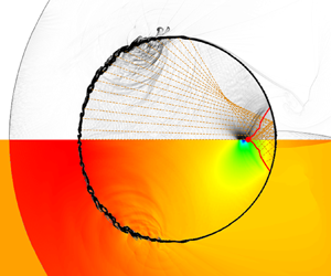
Numerical Investigation of Cylindrical Water Droplets Subjected to Air Shock Loading at a High Weber Number.
Fluids,
Vol. 10,
Issue. 4,
p.
81.