5 - Economic Impacts of an Investment Facilitation for Development Agreement

Summary

We quantify the impacts of a potential Investment Facilitation for Development (IFD) Agreement under negotiation at the World Trade Organization (WTO). The analysis is based on an innovative multiregion general equilibrium simulation model including bilateral representative firms. Consideration is given to foreign direct investment (FDI) and monopolistic competition. The model shows empirically relevant gains associated with removal of investment barriers in the form of transaction costs faced by foreign investors. The expected global welfare gains range between 0.56% and 1.74% depending on the depth of a potential IFD Agreement. The benefits are concentrated among the participants of the agreement with the highest welfare increase for the low-income and middle-income countries. Notable spillovers accrue to nonparticipants, which can be further increased by joining the agreement. Our results contribute to the relatively scarce research on investment facilitation and provide policymakers with information on the potential effects of the negotiated IFD Agreement.

5.1 Introduction

After the successful adoption of the Trade Facilitation Agreement (TFA) by the World Trade Organization (WTO) in 2014, investment facilitation has been gaining in popularity. Investment facilitation can be generally defined as a set of measures for improving the transparency and predictability of investment frameworks, streamlining procedures related to foreign investors, and enhancing coordination and cooperation between different stakeholders.¹ An Investment Facilitation for Development (IFD) Agreement was first suggested by a group of experts in 2015.² After three years of structured discussions on investment facilitation for development (2018–2020), the formal negotiations on a multilateral agreement started in September 2020 among more than 100 members of the WTO.³ An important component of the negotiations is an assessment of impacts, so members can rationalize their participation. Quantifying the impacts of the IFD Agreement is, at the outset, challenging. Despite the dynamic debate on investment facilitation, there is no generally accepted clear definition of the concept. Investment facilitation covers a wide range of areas with the focus on allowing investment to flow efficiently and for the greatest benefit. Transparency, simplicity, and predictability are among its most important principles. Moreover, investment facilitation refers to actions taken by governments designed to attract foreign investment and maximize the effectiveness and efficiency of its administration through all stages of the investment cycle. It does not, however, incorporate investment liberalization and protection, or investor–state dispute settlement. These issues remain a subject of bilateral and regional investment agreements.⁴

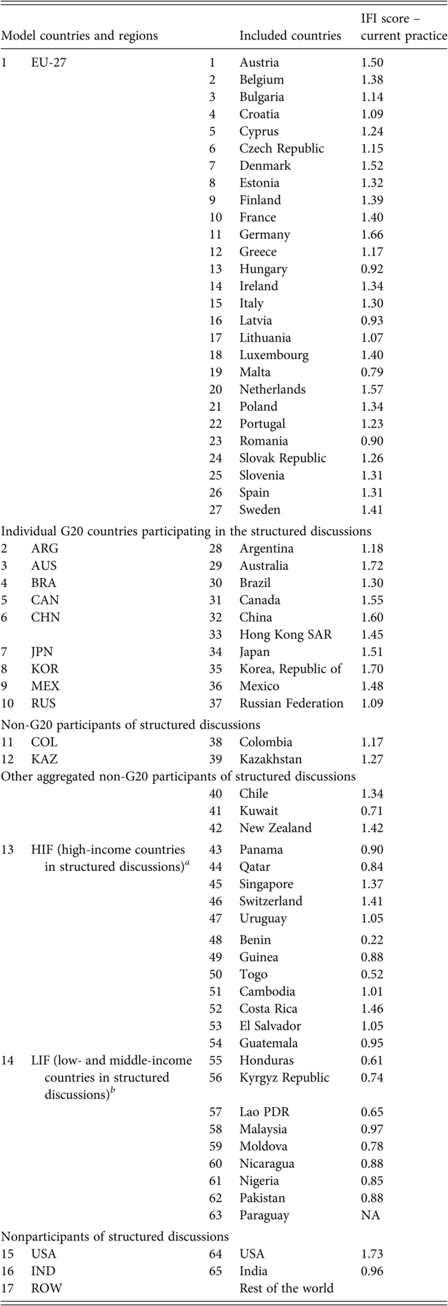
In this chapter, we use an economic model of global interactions to quantify the value of the IFD Agreement, given the outcomes of the structured discussions. The model is calibrated to GTAP 10 data characterizing trade and the social accounts. We aggregate the world into seventeen regions, including over sixty countries that participated in the structured discussions. We consider the possible IFD scenarios based on the Investment Facilitation Index (IFI) developed by Berger, Dadkhah, and Olekseyuk⁵ and Berger and Olekseyuk.⁶ The IFI helps to conceptualize the scope of investment facilitation along 6 policy areas and 117 individual measures and provides an indication of the level of current practice in investment facilitation across a large number of countries. It clearly illustrates that there are significant variations across countries and considerable gaps between the current practices of many countries as well as what might be considered best practice. The IFI score ranges from a low of 0.23 for Benin to a high of 1.73 for the United States (with an upper bound of 2.00). It is especially true that low- and middle-income countries would gain from implementing investment facilitation provisions. We use the IFI in this chapter to inform the quantitative level of the implied reduction of FDI barriers embodied in the IFD. While the absolute scale of the implied liberalization is uncertain, we leverage the IFI to establish a sound measure of the relative shocks across countries and regions. With the shocks specified, we use the economic model to establish plausible ranges for IFD benefits. The primary measure of the value of an IFD to different regions is reported from the model in terms of changes in economic welfare.⁷ We demonstrate the model’s operation as a tool for informing the policy debate, but we also warn that the model is sensitive to a set of critical assumptions. A continuation of the empirical research necessary to inform these assumptions is warranted.

To our knowledge, we are on the forefront of empirically quantifying the potential effects of the specific provisions of an IFD. Thus, we provide important and timely information at the point of policy formation. Our work provides results on the economic impact of a potential IFD on the most active countries during the structured discussions including Argentina, Australia, Brazil, Canada, China, Colombia, Japan, Kazakhstan, Mexico, Russia, South Korea, and EU-27. Other countries involved in the structured discussions within the WTO are aggregated into either the High-income Investment Facilitation (HIF) region or the Low- and middle-income Investment Facilitation (LIF) regions. Apart from members of the structured discussions, we also include the United States and India, major countries that are not participating in the WTO negotiations.⁸ At this level of geographic resolution, our country sample covers around 90 percent of world FDI stocks, with the rest of the countries aggregated into the rest of the world (ROW) aggregate region.

This chapter proceeds as follows. In Section 5.2, we describe the underlying data sources and the applied model of global trade. In Section 5.3, we outline the specific model scenarios and the implementation of the IFI-based shocks. Section 5.4 provides a set of results for all included countries and regions. In Section 5.5, we enumerate a set of critical ad hoc assumptions, and Section 5.6 illustrates the model’s sensitivity to our structural and parametric assumptions. Finally, in Section 5.7, we provide concluding comments and highlight follow-up research that would increase the precision of future quantitative measures of the value of investment facilitation.

5.2 Data and Model Description

The widely adopted Computable General Equilibrium (CGE) methodology provides valuable insights from policy reforms in different areas such as taxation, migration, trade and investment, development policy, climate change, carbon trading, food security, and anti-poverty policies. It is a standard tool of empirical analysis, which is broadly used for policy evaluation and advice. The method is able to capture economy-wide responses to proposed policy shocks. This approach allows for complex interactions of productivity differences at the country, sector, and factor levels, while accounting for shifts in demand as incomes change. International markets are impacted by changes in comparative advantage, trade flows, market entry, and resource reallocations following trade and FDI liberalization. CGE models simultaneously account for interactions among producers, households, and governments in multiple product markets and across several countries and regions of the world.

To quantify the impact of the IFD Agreement, we develop an innovative multiregion general equilibrium simulation or CGE model with four sectors (agriculture, manufacturing, services, and energy) and seventeen regions covering over sxity countries participating in the official negotiations (see Table 5.1 for country coverage and aggregation). The model extends the basic GTAPinGAMS structure presented by Lanz and Rutherford⁹ calibrated to Global Trade Analysis Project (GTAP) 10 data characterizing bilateral trade and the social accounts.¹⁰ Extensions include a consideration of FDI and imperfect competition in a multiregion setting following the model developed by Balistreri, Tarr, and Yonezawa.¹¹ Unlike that study, our model includes the ability to consider FDI in goods in addition to business services. For this purpose, we compute bilateral shares of foreign affiliate sales for model-specific sectors and regions using the data from Fukui and Lakatos¹² and the GTAP 9 data for 2007.¹³ Given the shares, we distinguish between goods and services supplied either by domestic firms or by foreign firms both operating in the host country (FDI case) and abroad (cross-border supply).

Table 5.1 Country coverage and regional aggregation

Model countries and regions			Included countries	IFI score – current practice
1	EU-27	1	Austria	1.50
		2	Belgium	1.38
		3	Bulgaria	1.14
		4	Croatia	1.09
		5	Cyprus	1.24
		6	Czech Republic	1.15
		7	Denmark	1.52
		8	Estonia	1.32
		9	Finland	1.39
		10	France	1.40
		11	Germany	1.66
		12	Greece	1.17
		13	Hungary	0.92
		14	Ireland	1.34
		15	Italy	1.30
		16	Latvia	0.93
		17	Lithuania	1.07
		18	Luxembourg	1.40
		19	Malta	0.79
		20	Netherlands	1.57
		21	Poland	1.34
		22	Portugal	1.23
		23	Romania	0.90
		24	Slovak Republic	1.26
		25	Slovenia	1.31
		26	Spain	1.31
		27	Sweden	1.41
Individual G20 countries participating in the structured discussions
2	ARG	28	Argentina	1.18
3	AUS	29	Australia	1.72
4	BRA	30	Brazil	1.30
5	CAN	31	Canada	1.55
6	CHN	32 33	China Hong Kong SAR	1.60 1.45
7	JPN	34	Japan	1.51
8	KOR	35	Korea, Republic of	1.70
9	MEX	36	Mexico	1.48
10	RUS	37	Russian Federation	1.09
Non-G20 participants of structured discussions
11	COL	38	Colombia	1.17
12	KAZ	39	Kazakhstan	1.27
Other aggregated non-G20 participants of structured discussions
		40	Chile	1.34
		41	Kuwait	0.71
		42	New Zealand	1.42
13	HIF (high-income countries in structured discussions)a	43 44	Panama Qatar	0.90 0.84
		45	Singapore	1.37
		46	Switzerland	1.41
		47	Uruguay	1.05
		48	Benin	0.22
		49	Guinea	0.88
		50	Togo	0.52
		51	Cambodia	1.01
		52	Costa Rica	1.46
		53	El Salvador	1.05
		54	Guatemala	0.95
14	LIF (low- and middle-income countries in structured discussions)b	55 56	Honduras Kyrgyz Republic	0.61 0.74
		57	Lao PDR	0.65
		58	Malaysia	0.97
		59	Moldova	0.78
		60	Nicaragua	0.88
		61	Nigeria	0.85
		62	Pakistan	0.88
		63	Paraguay	NA
Nonparticipants of structured discussions
15	USA	64	USA	1.73
16 17	IND ROW	65	India Rest of the world	0.96

Notes: This aggregation is based on the list of around seventy countries participated in structured discussions. The values for the IFI score are based on Berger, Dadkhah, and Olekseyuk (2021).

^a Macao SAR is a non-G20 high-income country that took part in the structured discussions; however, it is not included in this region as it is not separately available in the GTAP database. This country is represented in the ROW region.

^b This region does not include the following participants of the structured discussions: Liberia, Tajikistan, Montenegro, and Myanmar. These countries are not separately available in the GTAP database and constitute a part of the ROW region.

Given consistency of all other model features with the standard GTAPinGAMS formulation, we only document the extensions to the trade and FDI structures in this chapter.¹⁴ In this section, we briefly describe the two model structures explored: ARM, the perfect-competition Armington structure; and BRF, a monopolistic competition structure of bilateral representative firms.¹⁵

The agricultural (AGR) and energy (ENR) sectors are always modeled as perfectly competitive sectors with constant returns to scale (ARM). This standard modeling approach applies the Armington assumption of differentiated regional products to model foreign trade.¹⁶ In this framework, firm-level products and technologies are assumed to be identical within a region, whereas product varieties from different places of production are imperfect substitutes. Thus, agents consume domestic and foreign varieties of the same good, which are aggregated to a composite commodity using the so-called Armington elasticity of substitution. The assumption of homogeneous firm-level goods within one region is realistic for agricultural and energy products, which are usually characterized by rather low shares of intra-industry trade (i.e., below 60 percent) and rather high elasticities of substitution between different varieties, meaning that products are closer substitutes.

In contrast to agriculture and energy sectors, manufacturing (MAN) and services (SER) are modeled as monopolistically competitive sectors with FDI (BRF). In this model framework, we differentiate all goods and services on the firm level. The first application of the bilateral representative firms structure in a multiregion trade model is provided by Balistreri, Böhringer, and Rutherford.¹⁷ However, the authors do not consider FDI in their model specification. Thus, this is an important model extension necessary to investigate the effects of investment facilitation.

In general, contemporary trade models with monopolistic competition usually adopt either a Krugman¹⁸-style homogeneous firms structure or a Melitz¹⁹-style heterogeneous firms structure. We consider a hybrid model that is computationally tractable like the relatively simple Krugman model but includes bilateral selection of firms and rents associated with each market like the Melitz formulation. In a typical Krugman formulation, firms enter based on their profit opportunities across all markets. In our formulation, Krugman-style firms choose to operate, or not, in each foreign market. That is, there is an entry margin for every market. This captures the bilateral selection feature of the Melitz structure. We achieve a stable equilibrium with bilateral entry (selection) by designating a portion of observed capital payments to a bilateral specific-factor earning rents. Thus, the input cost for firms is increasing and varies across markets. Each good or service that is modeled under monopolistic competition is assumed to be provided by a small firm selling a unique variety. We characterize supply on a given bilateral cross-border trade link or supply through bilaterally designated FDI as provided by a bilateral representative firm (BRF).

Under investment facilitation, FDI barriers in the form of reduced transaction costs are diminished and more FDI firms enter. Overall output goes up, and there are additional gains through the normal variety (extensive margin) channel. Consumers obtain access to new varieties unavailable before IFD implementation, and producers gain from a higher number of intermediate goods and services. The entry condition of a representative firm is bilateral and, therefore, different from a standard Krugman formulation. In a standard Krugman formulation, the fixed cost of establishing a variety (entry) would be assumed specific to a given source region, and this cost would be covered by profits across all host markets. Relative to a standard Krugman model, therefore, the BRF formulation generates bilateral extensive-margin responses (like the selection effect in Melitz). In addition, because there is a specific factor, changes in bilateral distortions are properly allocated to those favored firms in the markets where they operate. For a more detailed description of the BRF formulation in an application, see Balistreri, Böhringer, and Rutherford, and for an extended discussion of monopolistic competition in computational simulation models,²⁰ see Balistreri and Rutherford.²¹

5.3 Investment Facilitation Scenarios

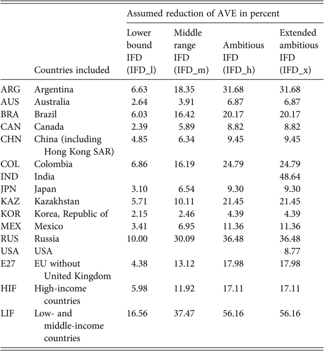
Following the detailed work on quantifying the current practice in investment facilitation as well as expected reforms due to an IFD Agreement by Berger, Dadkhah, and Olekseyuk,²² we use the country-level improvements in the IFI induced by different frameworks of the IFD Agreement as an assumption for the relative reductions in ad valorem equivalents (AVEs) of nontariff barriers (NTBs). Using this at an assumed scale, we are able to simulate several scenarios representing different depths and country coverage of the potential multilateral investment facilitation deal. The detailed assumptions about reductions of the AVEs are illustrated in Table 5.2.²³

Table 5.2 Policy shock assumptions under different IFD scenarios

	Countries included	Assumed reduction of AVE in percent
		Lower bound IFD (IFD_l)	Middle range IFD (IFD_m)	Ambitious IFD (IFD_h)	Extended ambitious IFD (IFD_x)
ARG	Argentina	6.63	18.35	31.68	31.68
AUS	Australia	2.64	3.91	6.87	6.87
BRA	Brazil	6.03	16.42	20.17	20.17
CAN	Canada	2.39	5.89	8.82	8.82
CHN	China (including Hong Kong SAR)	4.85	6.34	9.45	9.45
COL	Colombia	6.86	16.19	24.79	24.79
IND	India				48.64
JPN	Japan	3.10	6.54	9.30	9.30
KAZ	Kazakhstan	5.71	10.11	21.45	21.45
KOR	Korea, Republic of	2.15	2.46	4.39	4.39
MEX	Mexico	3.41	6.95	11.36	11.36
RUS	Russia	10.00	30.09	36.48	36.48
USA	USA				8.77
E27	EU without United Kingdom	4.38	13.12	17.98	17.98
HIF	High-income countries	5.98	11.92	17.11	17.11
LIF	Low- and middle-income countries	16.56	37.47	56.16	56.16

Source: Authors, cased on Berger, Dadkhah, and Olekseyuk (2021) and own calculations. The values for aggregate regions (CHN, E27, HIF, and LIF) are calculated as a GDP weighted average according to the mapping provided in Table 5.1 and using GTAP 10 data for weights.

Lower bound IFD (IFD_l): Investment facilitation measures are already, to some extent, included in different deep and comprehensive free trade agreements. Three recent FTAs, namely, The Comprehensive Economic and Trade Agreement (CETA) between the EU and Canada, the Comprehensive and Progressive Agreement for Trans-Pacific Partnership (CPTPP), and the United States–Mexico–Canada Agreement (UMCA), are reviewed in the initial IFI development.²⁴ In the agreements’ text, they identify commitments regarding investment facilitation such as horizontal transparency provisions (dissemination of regulations affecting foreign investment), digital signature, and protection of confidential information. These are mapped to the IFI and provide the improvements of index scores in accordance to each agreement. The results illustrate that the highest increase in the IFI score arises in case of a CPTPP-like IFD Agreement. For our lower-bound scenario, we use the percentage change in the IFI score according to the CPTPP agreement. Moreover, we assume that investment facilitation commitments covered by the regional treaty are multilateralized, so we apply them to all model-specific countries and regions that participated in structural discussions. Thus, a lower bound IFD simulation covers only a limited number of measures from the detailed IFI and suggests the lowest policy shocks ranging from a reduction of FDI barriers by 2.15 percent in South Korea to the highest reduction by 16.56 percent in low- and middle-income countries.

Middle range IFD (OFDM): We assume that commitments under the IFD Agreement follow closely Brazil’s circulated proposal for a possible WTO Agreement on investment facilitation (the “Model Agreement”),²⁵ which covers over 30 percent of investment facilitation measures included in the IFI (e.g., single window, focal point, and transparency provisions). Again, we map Brazil’s proposal from February 2018 and provide the change in IFI scores compared to the current practice, which is used in the simulation. We apply this policy shock to all included countries, except for India and the United States. Table 5.2 shows that the lowest decline of AVE occurs again in South Korea (2.46 percent), while the highest reduction of FDI barriers is assumed for the low- and middle-income countries (37.47 percent). Hereby, South Korea, Germany, and Australia will have the least changes in their investment facilitation rules since they have already adopted most of the commitments covered by this scenario.

Ambitious IFD (IFD_h): Given several submitted proposals during the structured discussions (by Brazil, Argentina, Russia, China, Kazakhstan, MIKTA, and FIFD),²⁶ we assume that commitments under the IFD include all mentioned investment facilitation measures, which strongly increases the coverage of measures included in the IFI (almost 50 percent of all measures) and reflects a much deeper reform potential. Most of the proposals have similar commitments in terms of transparency, predictability, fees and charges, and electronic governance. However, focal point commitments suggested by Argentina and Brazil and outward investment provisions suggested by China provide value added to the other proposals. In terms of magnitude, due to the broad coverage of measures, this scenario assumes the highest reduction of FDI barriers from 4.39 percent in South Korea up to 56.16 percent for the low- and middle-income countries (LIF region). In general, the low-income countries will gain most from implementation of investment facilitation provisions due to the low level of current practice and, consequently, the highest improvement in their IFI scores.

Extended IFD including United States and India (IFD_x): In this scenario, we also apply the highest reduction of FDI barriers following the ambitious scenario but extend the country coverage to India and the United States. For the United States, the shock is quite small (8.77 percent) since its practice in cooperation and electronic governance is even more advanced than the expected investment facilitation commitments. Only for focal point, application process, and transparency provisions, the IFI developers find some improvements in the IFI score. For India, in contrast, the ambitious IFD scenario would lead to significant improvements across all policy areas, with the highest increase by almost 70 percent for application process provisions. India’s overall shock for the ambitious scenario equals to 48.64 percent, the highest reduction of FDI barriers among all separately included countries (only for the aggregate LIF region, the value is higher with 56.16 percent).

5.4 Results

Conditional on the key assumptions, our model suggests significant gains from investment facilitation. Figure 5.1 reports the aggregated welfare²⁷ and Gross Domestic Product (GDP) impacts as percentage changes for the four scenarios. For the world as an aggregate, welfare increases range between 0.56 percent under the lower bound IFD and 1.74 percent under the ambitious scenario.²⁸ If India and the United States join the agreement, the potential gains would be even higher, with 2.46 percent. Consistently, the world GDP would also rise by 0.33 percent in case of lower bound IFD and over 1 percent in the ambitious scenarios (1.01 percent for IFD_h and 1.41 percent for IFD_x).

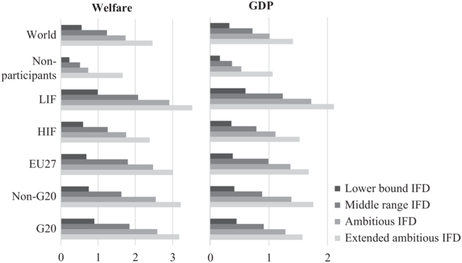
Figure 5.1 Aggregated regional welfare and GDP impact (percent).

Note: Table 5.1 provides country coverage for EU27, HIF, and LIF, which is identical with our model- specific regions. G20 covers all G20 countries involved in structured discussions (ARG, AUS, BRA, CAN, CHN, JPN, KOR, MEX, RUS). Non-G20 includes Columbia and Kazakhstan as participants of structured discussions. Nonparticipants include the United States, India, and the rest of the world.

Source: Authors.

In general, the results illustrate that the broader the coverage of the IFD Agreement and the higher the applied shocks, the higher are the gains. The benefits are concentrated among the regions participating in the negotiations,²⁹ with the highest proportional increase in welfare realized by the low- and middle-income countries (LIF) across all scenarios (0.99 percent for IFD_l and 2.91 percent for IFD_h). The other participating regions show somewhat lower welfare increases: In the middle range simulation (IFD_m), the values range between 1.26 percent for high-income countries (HIF) and 1.84 percent for G20 countries participating in the structured discussions. For the ambitious IFD scenario (IFD_h), the respective values equal to 1.75 percent (HIF) and 2.59 percent (G20). There are notable spillovers from applied investment facilitation reforms that accrue to regions not involved in the structured discussions. Their average welfare gains amount to 0.23 percent in case of IFD_l simulation and increase up to 0.73 percent in the IFD_h scenario. However, joining the agreement is beneficial not only for outsiders but also for all participating regions since they are able to generate higher gains (by approximately 0.6 percentage points), with the extended number of members in the IFD_x scenario.

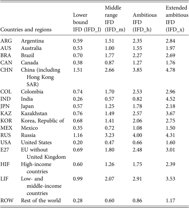
Table 5.3 reports the decomposition of the regional impacts for the individually modeled countries. We can see that China and Russia are the two countries gaining the most across all IFD scenarios. China’s welfare gains range between 1.51 percent in the lower bound simulation and 3.85 percent in case of ambitious IFD. Russia’s gains might be even higher, with 4 percent for the ambitious scenario, since this country starts with rather poor current practice, given the IFI score of 1.09. For the rest of individually included countries, the gains lie between 0.35 percent in Mexico (IFD_l) and 2.57 percent in Kazakhstan (IFD_h).

Table 5.3 Welfare impact (percent equivalent variation)

Countries and regions		Lower bound IFD (IFD_l)	Middle range IFD (IFD_m)	Ambitious IFD (IFD_h)	Extended ambitious IFD (IFD_x)
ARG	Argentina	0.59	1.51	2.35	2.84
AUS	Australia	0.53	1.00	1.55	1.97
BRA	Brazil	0.70	1.77	2.27	2.69
CAN	Canada	0.38	0.87	1.27	1.76
CHN	China (including Hong Kong SAR)	1.51	2.66	3.85	4.78
COL	Colombia	0.74	1.70	2.53	2.96
IND	India	0.26	0.57	0.82	4.52
JPN	Japan	0.57	1.25	1.78	2.18
KAZ	Kazakhstan	0.76	1.49	2.57	3.67
KOR	Korea, Republic of	0.68	1.41	2.06	2.75
MEX	Mexico	0.35	0.72	1.08	1.50
RUS	Russia	1.16	3.23	4.00	4.31
USA	United States	0.20	0.47	0.66	1.60
E27	EU without United Kingdom	0.69	1.80	2.48	3.01
HIF	High-income countries	0.60	1.26	1.75	2.39
LIF	Low- and middle-income countries	0.99	2.07	2.91	3.53
ROW	Rest of the world	0.28	0.60	0.86	1.17

Source: Authors.

Of particular interest is the fact that India, as a notable absentee in the structured discussions, has a lot to gain from investment facilitation reforms. Solely spillover gains reach 0.26 percent or even 0.82 percent under the IFD_l and IFD_h scenarios, which is comparable to some participating countries like Mexico or Canada in case of the IFD_m scenario. If India joins the agreement, welfare gains would rise strongly, with 4.52 percent under the IFD_x scenario. The United States, in contrast, does not show such a dramatic increase from participation: it is only moving from a spillover gain of 0.20 percent or 0.66 percent under the IFD_l and IFD_h scenarios to a 1.60 percent gain under the IFD_x simulation.

The reports of the percentage welfare changes are somewhat lower for larger developed regions (like the EU). This masks the value of an IFD Agreement in terms of dollars of benefits that accrue to these higher-income regions. Figure 5.2 reports the welfare increases in billions of dollars. We see that global welfare increases by more than US$250 billion under the lower bound scenario (IFD_l) and reaches more than US$1,120 billion in case of the extended ambitious IFD simulation. Hereby, substantial benefits accrue to the EU and other participating G20 countries. Participating G20 countries accrue 43–46 percent of the total global benefits across different IFD scenarios; for the EU, this share ranges between 24 percent (IFD_l) and 28 percent (IFD_m and IFD_h).

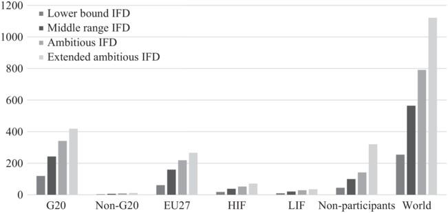
Figure 5.2 Aggregated regional welfare impact ($B).

Note: Table 5.1 provides country coverage for EU27, HIF, and LIF, which is identical with our model- specific regions. G20 covers all G20 countries involved in structured discussions (ARG, AUS, BRA, CAN, CHN, JPN, KOR, MEX, RUS). Non-G20 includes Columbia and Kazakhstan as participants of structured discussions. Nonparticipants include the United States, India, and the rest of the world.

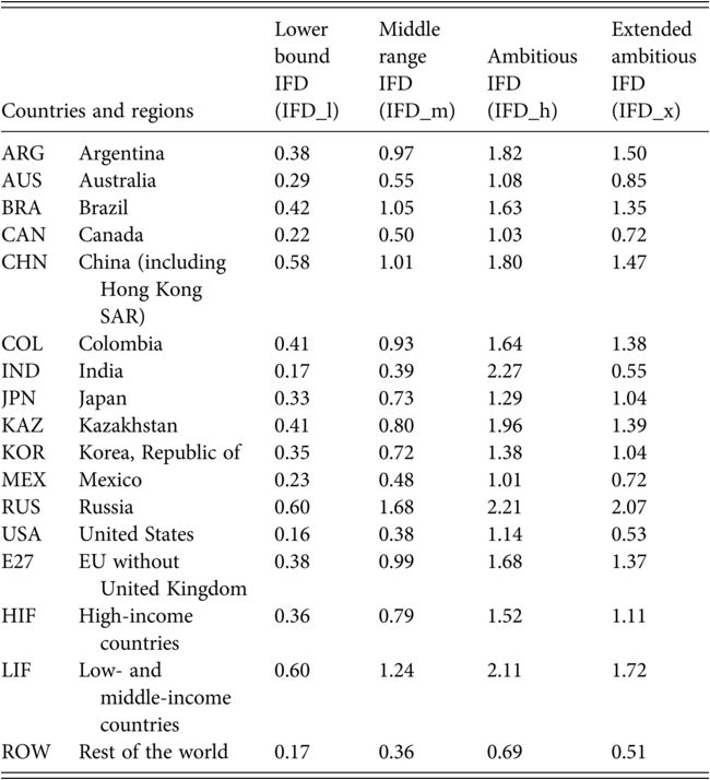
The model does report changes in GDP or regional incomes.³⁰ The country-specific GDP impact illustrated in Table 5.4 is generally consistent with the discussed welfare results. However, proportional changes in GDP tend to be somewhat smaller than welfare impacts because the basis is total income (including government spending and investment), whereas the basis for welfare is only private consumption. Table 5.4 and Figure 5.1 reflect this.

Table 5.4 GDP impact (percent)

Countries and regions		Lower bound IFD (IFD_l)	Middle range IFD (IFD_m)	Ambitious IFD (IFD_h)	Extended ambitious IFD (IFD_x)
ARG	Argentina	0.38	0.97	1.82	1.50
AUS	Australia	0.29	0.55	1.08	0.85
BRA	Brazil	0.42	1.05	1.63	1.35
CAN	Canada	0.22	0.50	1.03	0.72
CHN	China (including Hong Kong SAR)	0.58	1.01	1.80	1.47
COL	Colombia	0.41	0.93	1.64	1.38
IND	India	0.17	0.39	2.27	0.55
JPN	Japan	0.33	0.73	1.29	1.04
KAZ	Kazakhstan	0.41	0.80	1.96	1.39
KOR	Korea, Republic of	0.35	0.72	1.38	1.04
MEX	Mexico	0.23	0.48	1.01	0.72
RUS	Russia	0.60	1.68	2.21	2.07
USA	United States	0.16	0.38	1.14	0.53
E27	EU without United Kingdom	0.38	0.99	1.68	1.37
HIF	High-income countries	0.36	0.79	1.52	1.11
LIF	Low- and middle-income countries	0.60	1.24	2.11	1.72
ROW	Rest of the world	0.17	0.36	0.69	0.51

Source: Authors.

5.5 Critical Ad Hoc Assumptions

Computation of innovative models exploring new research questions like the impact of investment facilitation requires a substantial collection of data inputs. As this is a nascent attempt at quantification, we make some uncomfortable assumptions that will need to be addressed in future research. In the following, we present a set of critical assumptions made for the BRF calibration. Model results are conditional on (and sensitive to) these assumptions, which are not well informed by the data.

1. (1) Elasticity of substitution ($\sigma =3$): The elasticity of substitution across BRF varieties indicates the marginal value of a new variety. The lower is the elasticity, the more valuable is a new variety. Using the value adopted by Balistreri, Tarr, and Yonezawa³¹ for their FDI sectors, we assume an elasticity of three. This is generally on the lower end of many estimates, and so the expectation is that welfare impacts might be mitigated as the estimate is refined.

2. (2) The local supply elasticity of monopolistically competitive inputs ($\eta =1$): The supply elasticity indicates the degree to which firms can substitute away from the bilateral specific factor. The higher the elasticity, the more responsive output is, but the less revenues are allocated to the specific factor rents. The model is sensitive to this elasticity, with larger welfare gains for liberalizing regions under higher elasticities.

3. (3) For the SER (services) sector, we assume that 40 percent of observed cross-border provision is a specialized input for the associated multinational. That is, for example, an EU financial firm operating in Kenya will have specialized cross-border imports of financial services from the EU that are used to facilitate FDI supply. The specialized input formulation is developed by Markusen, Rutherford, and Tarr.³² While this parameter is necessary for an operational model, its measurement is difficult. Some limited information may be available from proprietary firm-level data.

4. (4) Since not all measures covered by the IFI induce costs to FDI firms, we make a scalar adjustment to the IFI of 0.05 to arrive at an actionable ad valorem model shock related to the IFD. Thus, we assume that 5 percent of the suggested reductions in investment barriers by the IFI (illustrated in Table 5.2) would lead to actual cost reductions for FDI firms. This scalar adjustment, by design, preserves the relative variation in the IFI across countries, but its level is uncertain. Conservatively, we consider at least 5 percent of the IFI as actionable under the adoption of an IFD. After applying the 5 percent adjustment, the FDI weighted average ad valorem shock across the participating countries under our middle range simulation (IFD_m) is 0.5 percent.

We consider other studies that have looked at FDI barriers to give some context to our conservative assumption that the actionable ad valorem model shock is derived by taking a fraction, 5 percent, of the reported IFI change. As a point of comparison, after applying the 5 percent adjustment, the FDI weighted average ad valorem shock across participating countries under our middle range simulation (IFD_m) is 0.5 percent. This is a small ad valorem shock in comparison to that observed in other quantitative studies of FDI liberalization. This gives us confidence that we are not exaggerating the economic impacts of the IFD. In the following section, we include a set of sensitivity runs that adopt a less conservative assumption by applying a scalar adjustment of 10 percent, effectively doubling the ad valorem shocks.

Other studies that investigated FDI barriers suggest much larger AVEs and often apply 25–50 percent of those as an actionable model shock. For example, based on information about regulatory regimes, Jafari and Tarr³³ develop a database on the barriers faced by foreign suppliers (discriminatory barriers) for 103 countries and 11 services sectors. They find that professional services (e.g., accounting, legal services) are among the sectors with the highest AVEs in high income countries (around 30 percent), but high-income countries have uniformly lower estimated AVEs than transition, developing or least developed countries. For instance, least developed countries (LDCs) exhibit the highest AVE in fixed line telephone services with an average of 764 percent (for thirteen countries in Sub-Saharan Africa and South Asia, the estimated AVE equals to 915 percent). For the rest of services sectors, the average AVEs for LDCs range between 3 percent for retail trade and 56 percent for rail transport.

There are also studies estimating the FDI barriers for single countries. For instance, Balistreri, Jensen, and Tarr³⁴ estimate and apply the AVEs of discriminatory and nondiscriminatory (apply equally to domestic and foreign firms) FDI barriers in services for Kenya. The values for nondiscriminatory barriers range between 2 percent for air transport and 57 percent for maritime transport. For discriminatory barriers, the upper bound is somewhat lower, with the highest AVE of 40 percent in maritime transport . For Belarus, Balistreri, Olekseyuk, and Tarr³⁵ use nondiscriminatory barriers between 5.3 percent in communications and 47.5 percent for water, rail, and other transport, while discriminatory barriers for the same sectors amount to 2.3 percent and 42.5 percent, respectively. Similar studies also exist for Armenia, Georgia, Kazakhstan, Malaysia, Tanzania, etc. and suggest a broad range for FDI barriers reaching over 90 percent (in Georgia and Kazakhstan) or even 100 percent (in Armenia).³⁶ Thus, assuming 25–50 percent of the described AVEs as an actionable model shock, our assumption seems to be quite conservative.

5.6 Sensitivity Analysis

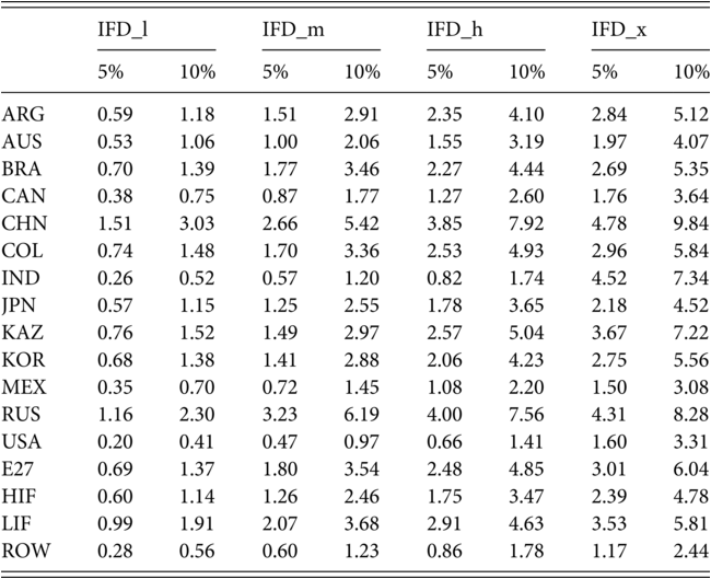
We proceed with a couple of exercises that illustrate the model’s sensitivity to our structural and parametric assumptions. Table 5.5 shows the comparison of welfare results under different assumptions of the scalar adjustment to the IFI, namely, 5 percent (our central assumption) and 10 percent. Since we prefer to be conservative in our central simulations, we would like to illustrate the magnitude of gains when we double the actionable ad valorem model shock related to the IFD. The results illustrate that a double scalar adjustment leads to welfare gains approximately twice as high as that in our central simulations. The global welfare increases by 1.11 percent under IFD_l and by 4.92 percent under IFD_x scenarios (compared to 0.56 percent and 2.46 percent in the central simulations, respectively). This corresponds to US$506 billion under the lower bound scenario and US$2,243 billion under the extended ambitious IFD.

Table 5.5 Sensitivity to different scalar adjustments to the IFI (percent equivalent variation)

	IFD_l		IFD_m		IFD_h		IFD_x
	5%	10%	5%	10%	5%	10%	5%	10%
ARG	0.59	1.18	1.51	2.91	2.35	4.10	2.84	5.12
AUS	0.53	1.06	1.00	2.06	1.55	3.19	1.97	4.07
BRA	0.70	1.39	1.77	3.46	2.27	4.44	2.69	5.35
CAN	0.38	0.75	0.87	1.77	1.27	2.60	1.76	3.64
CHN	1.51	3.03	2.66	5.42	3.85	7.92	4.78	9.84
COL	0.74	1.48	1.70	3.36	2.53	4.93	2.96	5.84
IND	0.26	0.52	0.57	1.20	0.82	1.74	4.52	7.34
JPN	0.57	1.15	1.25	2.55	1.78	3.65	2.18	4.52
KAZ	0.76	1.52	1.49	2.97	2.57	5.04	3.67	7.22
KOR	0.68	1.38	1.41	2.88	2.06	4.23	2.75	5.56
MEX	0.35	0.70	0.72	1.45	1.08	2.20	1.50	3.08
RUS	1.16	2.30	3.23	6.19	4.00	7.56	4.31	8.28
USA	0.20	0.41	0.47	0.97	0.66	1.41	1.60	3.31
E27	0.69	1.37	1.80	3.54	2.48	4.85	3.01	6.04
HIF	0.60	1.14	1.26	2.46	1.75	3.47	2.39	4.78
LIF	0.99	1.91	2.07	3.68	2.91	4.63	3.53	5.81
ROW	0.28	0.56	0.60	1.23	0.86	1.78	1.17	2.44

Source: Authors.

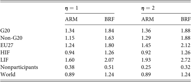
In Table 5.6, we consider the percentage welfare impact of the middle range scenario (IFD_m) under the central BRF monopolistic competition structure and under the full Armington treatment (under Armington, the MAN and SER sectors are treated as perfectly competitive).³⁷ The BRF structure does indicate substantially larger gains from the IFD. Across all regions, there are larger gains under the BRF structure, and even larger spillovers for the nonparticipating countries. On average, the gains are about 40 percent higher under BRF monopolistic competition. Our experience is that most of the added gains can be attributed to new variety gains. These extensive-margin gains are not available under the Armington formulation.

Table 5.6 Sensitivity across structural and parametric assumptions for the middle range IFD scenario (percent equivalent variation)

	$\eta =1$		$\eta =2$
	ARM	BRF	ARM	BRF
G20	1.34	1.84	1.36	1.88
Non-G20	1.15	1.63	1.29	1.88
EU27	1.24	1.80	1.45	2.12
HIF	0.94	1.26	0.92	1.26
LIF	1.60	2.07	1.93	2.72
Nonparticipants	0.38	0.51	0.25	0.32
World	0.89	1.24	0.89	1.24

Source: Authors

Calculating an exact attribution of the welfare gains from new varieties is challenging because in general equilibrium, the relative prices of varieties are in flux. The complex computation of variety gains, as suggested by Feenstra,³⁸ for example, applies in the context of a one-sector model without intermediate inputs. We can illustrate qualitative impacts, however, by reporting the weighted average change in entry of FDI varieties. In our central middle range scenario (IFD_m), the weighted average (across participating countries) increase in FDI manufacturing varieties is 0.3 percent, and the weighted average increase in FDI service varieties is 0.4 percent. This compares to no variety gains under the Armington treatment. New varieties in our central treatment translate directly into productivity and welfare gains by better fulfilling the needs of firms buying intermediates and consumption by households.³⁹

We emphasize that parametric sensitivity is also important. In Table 5.6, we also provide one example for the middle range scenario. Doubling the local supply elasticity (η = 2) increases the gains from the IFD for participants but mitigates the spillovers to nonparticipants (comparison of the BRF structure for $\eta =1$ and $\eta =2$). This is logically consistent. With a higher elasticity, the participants can take advantage of the liberalization, but it also means that nonparticipants can be more easily squeezed out of the market. Thus, competitive effects are exacerbated under higher elasticities.

5.7 Conclusion

In this chapter, we develop an innovative quantitative model for assessing the economic impacts of an IFD Agreement. We utilize the newly developed IFI⁴⁰ to inform model shocks and run scenarios consistent with the WTO structured discussions on investment facilitation. The model includes an innovative monopolistic competition structure and is calibrated to the GTAP 10 accounts. Our objective of including FDI in manufacturing and service sectors means that the data requirements exceed those available from GTAP. In particular, we need data that establish FDI stocks and the relationships between FDI firms and their home-country (specialized) inputs. A careful collection of these data is beyond the current scope of this chapter. Thus, our results rely on a set of key assumptions that will need to be addressed in future research.

Our model results generally illustrate that the deeper an IFD Agreement and the higher the applied shocks, the higher are the gains. For the world as an aggregate, welfare gains range between 0.56 percent under the lower bound IFD and 1.74 percent under the ambitious scenario. The benefits are concentrated among the countries that participated in structured discussions, with the highest increase in welfare realized by the low- and middle-income countries. Given their low level of current practice in investment facilitation and the highest policy shocks among all regions, these countries will be the biggest winners of a deep and comprehensive multilateral deal. In monetary terms, the expected gains of the low- and middle-income countries range between US$10 and US$30 billion depending on the depth of a potential IFD. Global gains may exceed US$790 billion, with substantial benefits for the EU (24–28 percent) and other participating G20 countries (43–46 percent).

Interestingly, there are notable spillover gains from applied investment facilitation reforms to countries taking no action under the agreement (between 0.20 percent and 0.82 percent). Joining a potential agreement is still very attractive to those countries with a low level of current practice in the field. Our extended ambitious IFD scenario with India and the United States among the members indicates significant benefits for India, with a welfare gain of 4.52 percent. The United States, in contrast, does not show such a dramatic increase from participation, with a welfare gain of 1.60 percent.

The presented results illustrate the potential impact of an IFD Agreement, which is closer to the lower bound for several reasons. First, even our ambitious scenario is still quite limited since it covers around a half of measures of IFI, which provides an in-depth concept of investment facilitation. If the IFD Agreement goes beyond measures covered in our policy shocks, the impact would increase. Second, a broader country coverage would also increase the global welfare gains. In this analysis, we focus on the list of countries that engaged in the structured discussions in the beginning of the process, while there are now over 100 countries taking part in the negotiations. Third, we prefer to be conservative in our central simulations, assuming a rather low ad valorem model shock. Our less conservative sensitivity runs (doubling the ad valorem shock) indicate much higher global welfare gains: 1.11 percent under the lower bound and 3.47 percent under the ambitious scenarios. This corresponds to US$506 billion under the lower bound scenario and almost US$1,580 billion under the ambitious IFD. Overall, our empirical results and, in general, the class of models employed suggest that the potential gains from an IFD significantly exceed those available from traditional tariff liberalization.

This analysis contributes to the very scarce research on investment facilitation and has the potential to provide policymakers with important information on the effects of the multilateral agreement. Applying the demonstrated model gives useful information on what instruments and the degree of investment facilitation commitments are needed to substantially enhance economic performance. It also provides a framework for considering the impacts and incentives for those countries that have chosen not to participate in the structured discussions.