1. Introduction
The length of life of individuals (longevity hereafter) is correlated with socio-demographic characteristics: on average women outlive men, and low-income individuals live, on average, significantly shorter lives than their better-endowed and wealthier peers (Olshansky et al., Reference Olshansky, Antonucci, Berkman, Binstock, Boersch-Supan, Cacioppo, Carnes, Carstensen, Fried, Goldman, Jackson, Kohli, Rother, Zheng and Rowe2012; Chetty et al., Reference Chetty, Stepner, Abraham, Lin, Scuderi, Turner, Bergeron and Cutler2016). Therefore, a pension system with a unique retirement age (or uniform contribution or replacement rates) is a priori problematic. Unaccounted longevity differences in contributory pension systems amount to taxing short-lived people and subsidising their long-lived peers (Ayuso et al., Reference Ayuso, Bravo and Holzmann2016), potentially distorting labour supply. Also, the social gradient in life expectancy reduces the progressivity of public pensions in those countries (e.g., the US) where the replacement rate is a negative function of earned income (Bommier et al., Reference Bommier, Leroux and Lozachmeur2011; Bosworth et al., Reference Bosworth, Burtless and Zhang2016). Some would even argue that longevity difference makes public pensions regressive (Piketty and Goldhammer, Reference Piketty and Goldhammer2015).
We show in this paper that unaccounted longevity differences violate the most basis definition of equity under both a Bismarckian (i.e., fully contributory) or a Beveridgian pension system.Footnote 1 One of the usual policy recommendations to address these problems is to differentiate the retirement age by socio-economic status (SES hereafter) (Leroux et al., Reference Leroux, Pestieau and Ponthière2015; Ayuso et al., Reference Ayuso, Bravo and Holzmann2016; Vandenberghe, Reference Vandenberghe2021). Related proposals recommend differentiating contributions or replacement rates (Bismarck) or the amount of the instalment (Beveridge) based on expected longevity differences. We explain later in the paper that these are functionally equivalent to retirement age differentiation. That is because, at its core, the problem of pension differentiation is an imperfect information problem. What is at stake is the difficulty/impossibility to fully individualize treatment (i.e., generate an almost infinite number of pension regimes) using a pension parameter (or a series of parameters) whose variation is intrinsically more limited than the realized longevity it is supposed to match. The degree of differentiation of pensions that can be achieved via pension parameters corresponds to what statisticians call the between-SES expected longevity differences. It leaves aside the (potentially very important) within-SES longevity heterogeneity. Given this imperfect information conundrum, we argue in this paper there might be another, possibly more effective, option to improve lifetime pension equity. We call it partial de-annuitization of public pensions.
Annuitization is a common (implicit) feature of most, if not all, public pension systems organized on a pay-as-you-go basis (PAYG).Footnote 2 But in principle, if we leave aside liquidity and transition issues,Footnote 3 nothing prevents imagining a public PAYG pension scheme where part of the sums earmarked for someone are paid upfront (i.e., at beginning of the retirement spell) as a lump sum.Footnote 4 In the universe of fully funded pensions systems, including public or publicly sponsored ones, that option is available, and sometimes explicitly related to the perspective of a short life. Examples that we are aware of comprise
• The Netherlands. From 2023 onward, the Dutch Government will allow lump sum payments equal to a maximum of 10% of the accumulated capital when reaching the retirement date, under occupational pension plans (Dillingh and Zumbuehl, Reference Dillingh and Zumbuehl2021).
• The US, State of New York where the public sector employees can upon retirement fill a form to receive a ‘Partial Lump Sum Payment’ corresponding to 5 to (max) 25% of the accumulated capital, with ‘a reduced lifetime monthly benefit based on the remainder’(New York State Government, 2022).
• The UK, you may be able to take all the money in your occupational pension as a tax-free lump sum, if (…) you're expected to live less than a year because of serious illness, you're under 75, and you do not have more than the lifetime allowance of £1,073,100 in pension savings (UK Government, 2022).
• Canada, British Columbia, with the Public Service Pension Plan you may receive a lump-sum payment in lieu of a monthly pension if you have an illness or disability that has shortened your life expectancy (British Columbia Government, 2022).
In what follows, partial de-annuitization will not be an option but considered as automatic and universal (i.e., applicable to all pensioners). But the key intuition will remain the same as in the above UK or Canadian examples: if longevity varies and is a source of inequality, paying part of the accrued pension rights when (all) prospective pensioners are still alive is a way to minimize pension-related lifetime inequalities. The idea is echoing the notion of reverse retirement introduced by Ponthiere (Reference Ponthiere2020) who considers a model where individuals start their life in retirement (and thus ‘all’ receive their pension) before moving to work. What follows should be seen as a milder, but more realistic, version of that thought-provoking idea. Ours is more related to the notion of front-loaded annuities or benefits in pension economics (Palmer, Reference Palmer2000; Brown, Reference Brown, Feldstein and Liebman2002).Footnote 5
Our realism also stems from the fact that we are not so much interested in the absolute level of lifetime equity gains that can be achieved via de-annuitization. It is almost tautological that full de-annuitization is very effective in dealing with longevity differences. But also that it would annihilate pensions' capacity to cover the longevity risk.Footnote 6 Our perspective in this paper is that of the relative performance of de-annuitization vs. retirement age differentiation (and by analogy, vs. differentiation policies targeting either the contributory phase or the payout phase of pensions (Sanchez-Romero et al., Reference Sanchez-Romero, Lee and Prskawetz2020)). The key question of this paper is how much de-annuitization is needed to match the equity gains delivered by retirement age differentiation?
Of course, for obvious budgetary reasons, introducing de-annuitization (and the upfront payment of a lump sum to all) implies a reduction of the value of the pension annuity. Answering the question of how much de-annuitization is needed is thus also a way to quantify the propensity of partial de-annuitization to come at the expense of one of the key objectives of annuitization, i.e., insuring individuals against the risk of longevity. That risk – and the underlying shortsightedness of individuals – is regularly mentioned in the literature as a justification for the State to impose a minimal degree of annuitization of the pension capital (Barr and Diamond, Reference Barr and Diamond2006).
The results presented in this paper show that the reduction of the monthly instalment needed to match the equity gains achieved via extensive retirement age differentiation (up to 200 different ages) is quite small. As far as we know such a result is a novelty and constitutes the key contribution of this paper to the economic literature on pensions and annuities.
Using US data assembled by Chetty et al. (Reference Chetty, Stepner, Abraham, Lin, Scuderi, Turner, Bergeron and Cutler2016), we estimate it to be about 4%, and the corresponding payment of an upfront lump sum to correspond to a bit less than a full year of benefits. The modest reduction of the annuity suggests a limited risk of significantly eroding pensions' monthly payment adequacyFootnote 7 and their capacity to insure the risk of longevity. Also, partial de-annuitization is administratively less costly to implement than retirement age differentiation. It does not require an upstream statistical analysis of the determinants of longevity. And it does not force civil servants to systematically verify pensioners' SES category (which, given the stakes for the retirees might be prone to misreporting). We also anticipate less legal challenges. De-annuitization amounts to treating everyone equally. By definition, this is not the case of retirement age differentiation. Just consider the idea of differentiating the age of retirement by gender to account for the well-documented gender longevity gap?Footnote 8 Would that be considered as legally acceptable? For instance, a look at the jurisprudence of the European Court of Justice suggests that the answer is simply no.
Note that throughout this paper will we consider that retirement age(s) or the degree of de-annuitization is decided paternalistically by the State. Such a perspective partially reflects the European context underpinning this paper, where retirement is still largely driven by State-edicted rules. This said, we also consider the political economy of the proposal, i.e., that of the number of people who could support it.
From a normative point of view, we will consider throughout the paper that all realized longevity differences matter. This means that we subscribe to ex post egalitarianism when it comes to dealing with longevity inequalities (Fleurbaey et al., Reference Fleurbaey, Leroux, Pestieau and Ponthière2016).
The rest of the paper is organized as follows. Section 2 exposes a simple framework to assess the gains from retirement age differentiation. Section 3 does the same thing for the idea of de-annuitization and exposes how the two approaches are logically related. Section 4 exposes the longevity data we use. Section 5 presents the key numerical results of the paper. Section 6 examines the political economy of partial de-annuitization considering the number of winners vs. losers. Section 7 concludes with a discussion of the policy context and feasibility of partial de-annuitization.
2. A simple framework to assess the equity gains of retirement age differentiation
We consider a world where longevity varies significantly across individuals forming a cohort (l i, i = 1…N) and in a way that is related with observable SES category j, with j = 1…k and n j the number of individuals forming category j. Logically we have that $\sum _{j = 1}^k n_j = N$![]() . The full distribution of longevity is unknown to the planner/pension minister. Her knowledge is limited to the correlation between SES and longevity. Equivalently, the planner can only differentiate treatment (retirement age) based on the j = 1…k SES group to which individuals belong.
. The full distribution of longevity is unknown to the planner/pension minister. Her knowledge is limited to the correlation between SES and longevity. Equivalently, the planner can only differentiate treatment (retirement age) based on the j = 1…k SES group to which individuals belong.
Throughout the paper, we consider the two canonical versions of PAYG public pensions: the fully contributory Bismarckian version where benefits are indexed on contributions, and the Beveridgian one where every individual receives the same pension.
2.1 Bismarckian contributory pension scheme
The problem of policymakers under such a regime is to equalize the actuarial fairness ratio (afr) of lifetime pension benefits to lifetime pension contributions.Footnote 9 Abstracting from education length differences, career breaks, wage growth, demographic changes or discount and indexation rates, and considering that retirement age is uniform, that actuarial fairness ratio writes,

Centrally defined reference retirement age is ra and lifetime benefits are equal to the time spent in retirement times the annuity δw i,j where δ is the replacement rate and w i,j is the individual level of earnings. Note that people can die before reaching retirement age. So we have the dummy variable S i,j(ra) = 0 if l i,j ≤ ra and S i,j(ra) = 1 otherwise. By definition of a Bismarckian system, lifetime contribution corresponds to the duration of the career (here, the retirement age) that multiplies the annual contributions at a rate η. We define θ ≡ (δ/η) as the (uniform) rate of replacement for each euro of contribution.Footnote 10
An alternative way of expressing reference retirement age is ra ≡ α l where l is the unique reference longevity and 0 ≤ α ≤ 1 is the share of life the reference person is supposed to spend working. Reference retirement age and reference longevity are thus isomorphic formulations in our setting.
The equalization of lifetime ratios across individuals ($\forall i, \;j\;\colon \;afr_{i, j} = afr$![]() ) can be achieved via the full individualization of the retirement age, or, equivalently, via the use of each individual's longevity l i,j when defining the retirement age.Footnote 11 For any value of α, if the retirement age is fully individualized (i.e., $ra_{i, j}\equiv \alpha \; l _{i, j}, \;\;\forall i, \;j$
) can be achieved via the full individualization of the retirement age, or, equivalently, via the use of each individual's longevity l i,j when defining the retirement age.Footnote 11 For any value of α, if the retirement age is fully individualized (i.e., $ra_{i, j}\equiv \alpha \; l _{i, j}, \;\;\forall i, \;j$![]() ), we verify
), we verify
Note that, by definition, if the retirement age is fully individualized, and if α < 1,Footnote 12 S i,j() is always equal to 1. In other words, nobody dies before reaching his fully individualized retirement age.
Using a uniform reference retirement age (i.e.,ra ≡ α l) introduces a gap between the fair ratio and the actual one
or equivalently when the reference retirement age is differentiated by SES category (i.e.,raj ≡ α lj), the (presumably smaller) gap is
A graphical representation of what happens under uniform vs. differentiated retirement age appears on Figure 1. The lower part of the graph represents the distribution of realized longevity, while the upper part depicts the (lifetime) actuarial fairness ratio (afr ij). The first-best situation amounts to ensuring that every person gets the same ratio corresponding to the horizontal dashed line. The achieved degree of actuarial fairness corresponds to the solid and doted rising lines. Under uniform retirement age (solid rising line), only those whose longevity coincides with reference longevity (l) get the first best. All the others get less or more than what lifetime equality commands. Those who reach that retirement age but die before the reference longevity l get less than what they should. And those whose longevity exceeds l get too much. Under differentiated retirement age (two different retirement ages are depicted in Figure 1 and correspond to the dotted rising lines), the number of people who get exactly what equity commands (i.e., those whose longevity corresponds to the intersection between the dashed and doted lines) rises. Also the integral of the distances between the doted lines and the dashed horizontal line become lower, reflecting a reduction of the inequity gaps in Equation (3). However, situations synonymous with afr i,j ‘undershooting’ or ‘overshooting’ still abound.
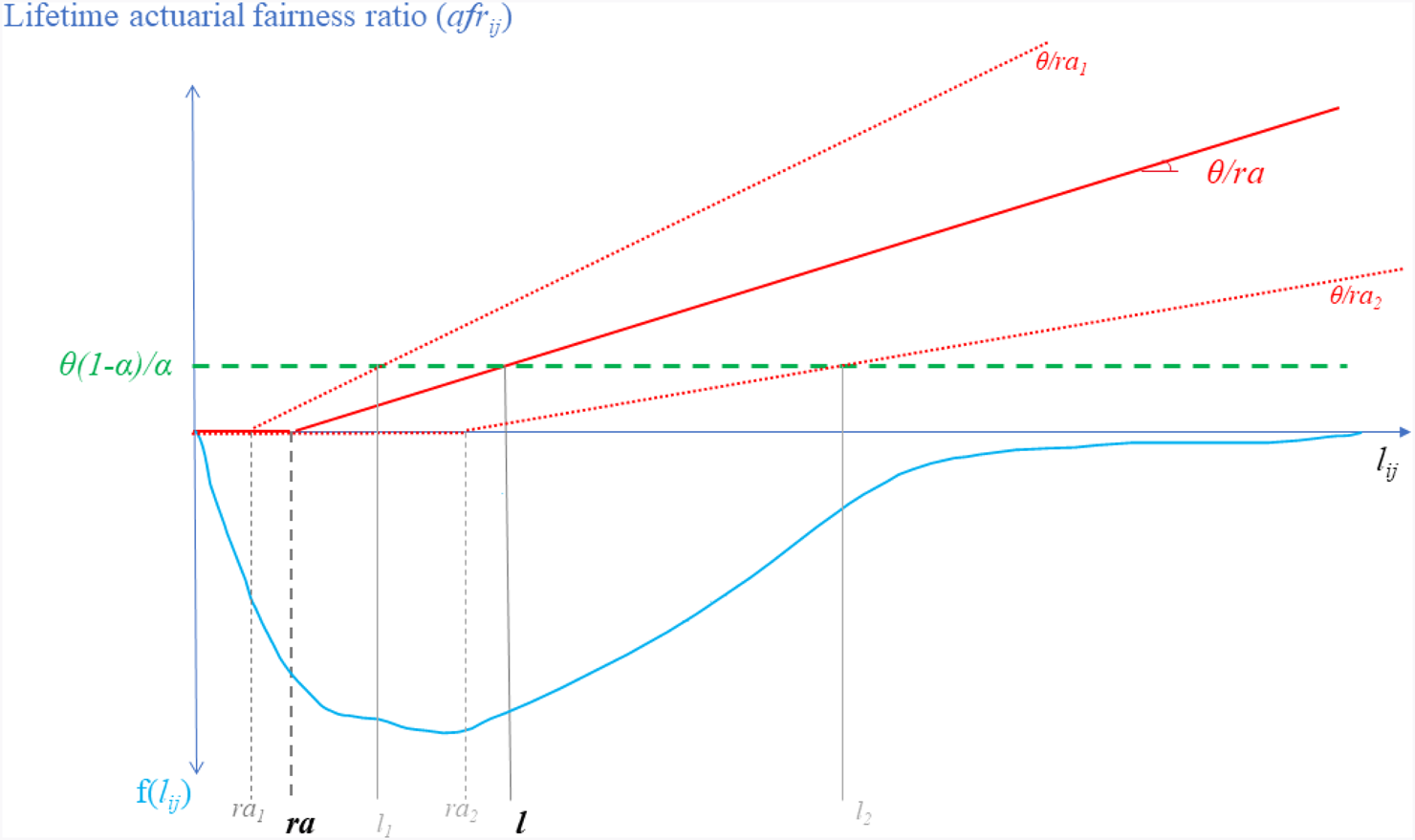
Figure 1. Bismarckian pension under uniform vs. diff. ret age.
Note that Figure 1 also reveals what would happen if, instead of differentiating the age or retirement, policy makers were to differentiate by SES either the contribution rate η or the replacement rate δ. That would amount to differentiating θ ≡ (δ/η), thus the slope of solid line, while keeping the retirement age unchanged (i.e., uniform). Instead of relying on raj to (try) to reflect realized longevity differences (i.e., any value on the horizontal axis), the planner would use θ j. More specifically, while here we explore what happens when raj becomes a positive function of expected longevity, in an alternative (but fairly equivalent approach) one could examine what happens were θ j to become a negative function of expected longevity. And echoing the point we raised in the introduction, it is likely that the outcome of that type of differentiation would not fundamentally change. That is because, at its core, the problem of pension differentiation is an imperfect information problem. How to fully individualize (and thus generate an almost infinite number of pension regimes), using only a limited number of values for the pension parameters (ra, θ, δ, η) mirroring the equally limited number of expected longevities (one for each SES j = 1…k) the policy maker knows? And combining several parameters of differentiation (i.e., simultaneously differentiating ra and θ for instance) would not bring much of change either, because the information used to implement that ‘hybrid’ approach of differentiation would still boil down to exploiting a mere correlation between SES category k and realized longevity.
Following Baurin (Reference Baurin2021), the overall reduction in the propensity of retirement policy to deviate from the full individualized first best can be expressed as an indexFootnote 13 ∈[0, 1] where the numerator aggregates the (absolute) values of the individual equity gaps under retirement age differentiation by SES j = 1…k, and the denominator does the same when there is no differentiation. Note that the index being a ratio, constant θ cancels out. In the numerical simulations underpinning results of Section 4.2 the differentiated reference retirement ages/longevities correspond to averages by SES category j.

Note finally that retirement age differentiation can generate budgetary savings (thus a surplus) in comparison with uniform retirement. This is because the overall (or average) time spent in retirement may go down. What is more, with a Bismarckian regime, the money not spent on those who live longer is likely to outweigh the cost of financing early retirement to the benefit of the short-lived individuals. In what follows we will assume that the planner absorbs the net budgetary surplus generated by the move from uniform to differentiated retirement age. An alternative is to enforce cohortal budget equivalence, i.e., to use the surplus to increase the replacement rate θ in the numerator of our (in)equity index Equation (6). We explore that alternative in detail in Appendix A2. But the key result is that the equity gains achievable via retirement age differentiation are likely to be lower. This is because the time component of the equity gaps (Equation (5)) – that inevitably still exists under retirement age differentiation – is priced at a higher rate.Footnote 14 Say differently, in the equity indexFootnote 15, the time component of the gaps in the numerator is now multiplied by a higher θ than in the denominator.Footnote 16 Thus the equity gains achieved in terms of years spent in retirement are eroded by the (remaining) year gaps weighing more in monetary terms.
2.2 Beveridgian pension scheme
By definition, a Beveridgian pension system would rather aim at equalizing lifetime pension benefits (B i,j).
In the above expression, b is the standard uniform annual/monthly pension (which is independent of earning w i,j and contributions) that multiplies the time spent in retirement. Again, people can die before reaching retirement age. So we have the dummy variable S i,j(ra) = 0 if l i,j ≤ ra and S i,j(ra) = 1 otherwise. Equalization of lifetime benefits ($\forall i, \;j\;\colon \;B_{i, j} = B$![]() ) can only be achieved via full-individualization of retirement age, or the corresponding reference longevity (ra ij ≡ l i,j − κ), where κ is the reference number of years spent in retirement.
) can only be achieved via full-individualization of retirement age, or the corresponding reference longevity (ra ij ≡ l i,j − κ), where κ is the reference number of years spent in retirement.
Note again that S i,j() = 1 if there is perfect individualization and if κ > 0. We logically assume κ is the time spent in retirement by the person whose longevity is equal to the reference longevity (l) under a uniform retirement policy (κ = l − ra = (1 − α)l).Footnote 17
Key is that the use of a uniform retirement age/longevity reference (ra) leads to lifetime benefit gaps
or equivalently when the reference retirement age is differentiated by SES category (raj), the (presumably smaller) gap is
Again, we can produce a graphical representation of what is at stake under uniform vs. differentiated retire. It is to be found in Appendix A1. In more analytical terms, the reduction in the overall propensity of retirement policy to deviate from the fully individualized first best can be expressed as the following index, where the constants b cancel out

Note again that, so far, we have assumed that the planner absorbs any net surplus/deficit generated by the move from uniform to differentiated retirement. The alternative policy would be to raise(reduce) b prorata in the numerator of the (in)equity index equation (11), and enforce cohortal budget equivalence. Under a Beveridgian regime, retirement age differentiation is likely to generate a surplus(deficit) if the overall time spent in retirement goes down(up). Not absorbing that surplus(deficit) means that policy makers raise(reduce) b. This again means that year equity gaps – that still exist under retirement age differentiation – are ‘priced’ differently. Thus the equity gains achieved in terms of years spent in retirement are eroded(amplified) by the (remaining) year gaps weighted differently. This translates into different equity gains than those reported in result Section 4.2. We analyse this cohortal-budget-equivalence alternative in detail in Appendix A2. Results, in short, suggest that under a Beveridgian regime retirement age differentiation could generate a (small) surplus, allowing for a (slightly) higher b.Footnote 18 Thus, again, our main results in Section 4.2 (derived without imposing cohort budgetary equivalence) should be seen as an upper bound of the achievable equity gains.
To sum up, minimizing both the Bismarckian and Beveridgian inequity indices (Equations (6) and (11)) depends on the social planner being able to match the full distribution of longevity across individuals l i,j, i.e., the different values of the horizontal axis forming the longevity distribution on the lower part of Figures 1 and A1. If she can only go for tagging (Akerlof, Reference Akerlof1978), i.e., use j = 1…k < N proxies lj that are simply correlated to realized longevity l i,j to differentiate treatment, and if unaccounted longevity differences are important and matter, then both policies should translate into values of our indices that are relatively close to 1. In Section 4.2, we will show simulation results illustrating this, using US data on longevity heterogeneity.
3. De-annuitization
We now consider Bismarckian and Beveridgian pension schemes with some de-annuitization: i.e., with an upfront lump-sum payment LS.Footnote 19 With the Bismarckian pension, the actuarially fair ratio becomes

with the (logically lower) annuity corresponding here to a lower replacement rate, i.e., δ ′ < δ, θ ′ ≡ (δ ′/η) < θ, and $\mu \equiv ( {LS_{i, j}/{\boldsymbol ra} \eta w_{i,\, j}} ) , \; \forall i, \;j$![]() . Note that the lump sum paid varies for each individual, but it is strictly proportional to lifetime contributions, guaranteeing that each individual achieves some positive uniform (up-front) ratio.Footnote 20 And it is that uniform μ that contributes to reducing equity gaps in Equation (14) below. In Appendix A3 we show that the value of μ that is compatible with the budget-equivalence constraint (i.e., same sums spent on a cohort with and without de-annuitization) is
. Note that the lump sum paid varies for each individual, but it is strictly proportional to lifetime contributions, guaranteeing that each individual achieves some positive uniform (up-front) ratio.Footnote 20 And it is that uniform μ that contributes to reducing equity gaps in Equation (14) below. In Appendix A3 we show that the value of μ that is compatible with the budget-equivalence constraint (i.e., same sums spent on a cohort with and without de-annuitization) is
where the term that post-multiplies (θ − θ ′) is the ratio of the (wage weighted) number of years spent in retirement to the (wage weighted) number of years spent contributing. As to the denominator remember that N is the size of the cohort of pensioners considered and $\bar{w}$![]() the average wage earned by the members of that cohort. Note finally that μ > 0 if θ ′ < θ.
the average wage earned by the members of that cohort. Note finally that μ > 0 if θ ′ < θ.
The interesting point is what happens with the inequity gap indices when θ is reduced to θ ′. The building blocks of the Bismarckian version of that index consist (to the numerator) of the gaps between the actuarially fair and the one achieved via the policy envisaged. With de-annuitization (assuming a unique retirement age), the gaps become

The index capturing the gains achieved via de-annuitization (the reference policy being one with no de-annuitization and uniform retirement age) now writes:

Crucial is that the gain achieved via de-annuitization is strictly proportional to the reduction of the annuity ((θ ′/θ) < 1).Footnote 21 Thus an interesting numerical exercise, based on actual longevity data, is to compute the gains that can be achieved via retirement age differentiation. This will provide a certain value of the index I Bismark < 1, from which we can infer the corresponding value of (θ ′/θ) (and thus also of μ) ensuring the same fairness improvement. Thus, quantifying the gains that can be achieved via retirement age differentiation – as we do in Section 4.2 – amounts to computing the degree de-annuitization that will provide exactly the same pension fairness gains.
A similar equivalence can be established between retirement age differentiation and partial de-annuitization of Beveridgian pensions. This time, the lump sum LS paid upfront is the same for every individual (hence the absence of subscripts i, j) and writes:
with a logically lower annuity b ′ < b. In Appendix A3 we show that the value of LS that is compatible with the budget-equivalence constraint (i.e., same sums spent on a given cohort with and without de-annuitization) is
where the term that post-multiplies (b − b ′) that is just the average number years spent in retirement. Note that LS > 0 if b ′ < b.
The key point is again to consider what happens with the indices exposed above when b is reduced to b ′. The building blocks of the Beveridgian version of that index consist (to the numerator) of the gaps between the fair annuity and the one actually achieved via the policy envisaged. With de-annuitization (assuming again a unique retirement age), the gaps become
Hence the index capturing the gains achieved via de-annuitization (the reference policy still being one with no de-annuitization and uniform retirement age) writes

So, paralleling the result for Bismarckian pensions in Equation (15), we see that the gains achieved here via de-annuitization are strictly proportional to the reduction of the annuity ((b ′/b) < 1).
4. Data and results
4.1 Data construction
The data used to analyse partial de-annuitization vs. retirement age differentiation are from the US. They consist of a simulation of the full distribution of longevity across a cohort of N individuals with different socio-demographic background (l i,j; i = 1…n j; j = 1…k) who have survived until prime age. As its core, the simulation rests on the (unavailable to us) mortality rates assembled by Chetty et al. (Reference Chetty, Stepner, Abraham, Lin, Scuderi, Turner, Bergeron and Cutler2016).
The underlying micro data comprise a sample of 1.4 billion observations from anonymized tax records, covering the years 1999–2014. Mortality data start at age 40 and are available either by gender, US state of residence and income quartile; or by gender and income percentile. We retain the gender × income version of the Chetty data. More precisely, we use the (publicly available) parameters of Gompertz functions they provide for each gender × income cell j, alongside the number of people in the US population belonging to these cells (n j, j = i…k).Footnote 22 The parameters of the Gompertz function capture the expected differences of mortality between categories j. Whereas the predicted values delivered by each Gompertz function j provides the ‘within’ category distribution of mortality rates for each (potential) age of death.Footnote 23 These mortality rates by age can then be multiplied by the number of individuals forming each cell j to know the number of individuals whose longevity is equal to 40, 41, …, 120.
In Figure 2 we display the Gompertz-generated distribution of longevity for men belonging to the lowest income percentile of the US male population vs. the equivalent distribution for women forming the highest income percentile of the female population. Expected/average longevity (corresponding to the dashed vertical lines) varies between the two groups: the expected longevity gap is larger than 16 years (88.7 vs. 71.9 years). Still, the solid curves capturing the full distribution of realized longevities within each group reveal that quite many women forming the upper income percentile die before the average age of 88.7 (and would deserve to retire early), while some for low-income men live beyond that age (and to not deserve to early retire).Footnote 24
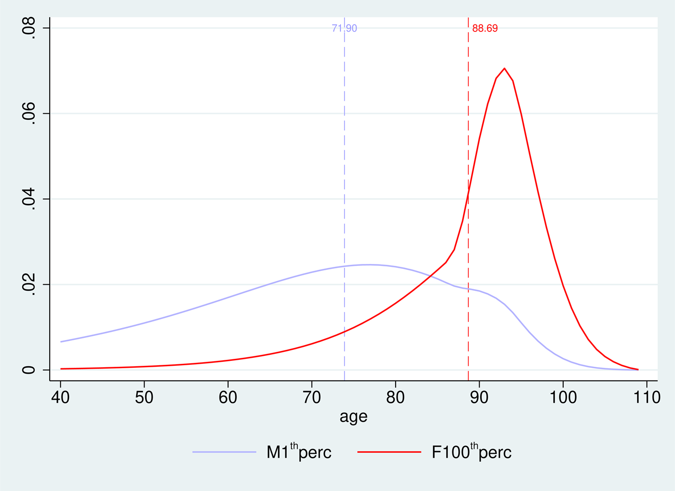
Figure 2. USA-[M]ale lowest income percentile and [F]emale highest percentile; expected/average longevity difference between the two groups vs. full distribution of realized longevities within these groups. Source: Chetty et al. (Reference Chetty, Stepner, Abraham, Lin, Scuderi, Turner, Bergeron and Cutler2016), based on mortality data beyond the age of 40.
4.2 Numerical simulation results
We start by assuming that our reference longevity (i.e., l) underpinning the uniform retirement policy is the average longevity in the Chetty data. Without loss of generality, and for the sake of clarity, the value of the share of life spent in employment α is chosen so that the corresponding uniform retirement age is equal to 65. Here after, the results for the retirement age policy are centred on that age of 65 (ra = 65).
Given the Chetty data documenting longevity differences only past the age of 40, the minimal retirement age under retirement age differentiation is 40. And with de-annuitization, the lump-sum payment is also assumed to intervene at 40. By definition, it consists of paying a lump-sum to all whose longevity is considered, and that is only feasible before the first individual dies, thus here at 40.Footnote 25 Also, given the data used, the two policies examined here (equally) ignore the problem of the very short-lived, i.e., those who don't survive up to the age of 40. Note that the hypothetical use of a data set documenting longevity only from the age of 50 or 55 would simply inflate the number of individuals who are de facto not compensated, but without affecting our key analytical results markedly. Remember that our prime interest is to assess de-annuitization needed to match whatever can be achieved via retirement age differentiation, and by that we also mean the extent to which that policy ignores some short-lived. Remember also that the major factor driving our results is the (in)ability of the planner to match the full distribution of longevity using a few proxies. Whether it is the post 40, 50 or 55 distribution does not matter much.
Our results consist of the simulated values of the gains generated by retirement age differentiation in terms of inequity gap indexes exposed in Equations (15) and (19), one for the Bismarckian system and one for the Beveridgian one. In both cases we estimate numerically the gains achieved by resorting to 200 different reference retirement ages/longevities (i.e., j = 1…200, corresponding to 2 genders × 100 income percentiles). The differentiated retirement ages we use are visible in Figures 3 and 4. They correspond to each of our SES categoryj's average longevity (multiplied by α with Bismarck, or minus κ with Beveridge).
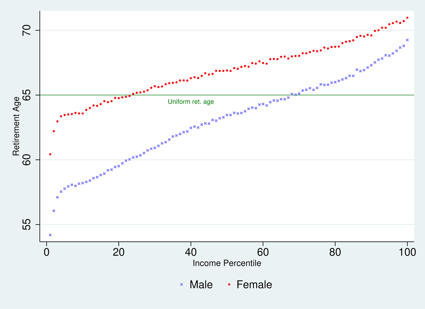
Figure 3. Bismarckian differentiated pension ages.
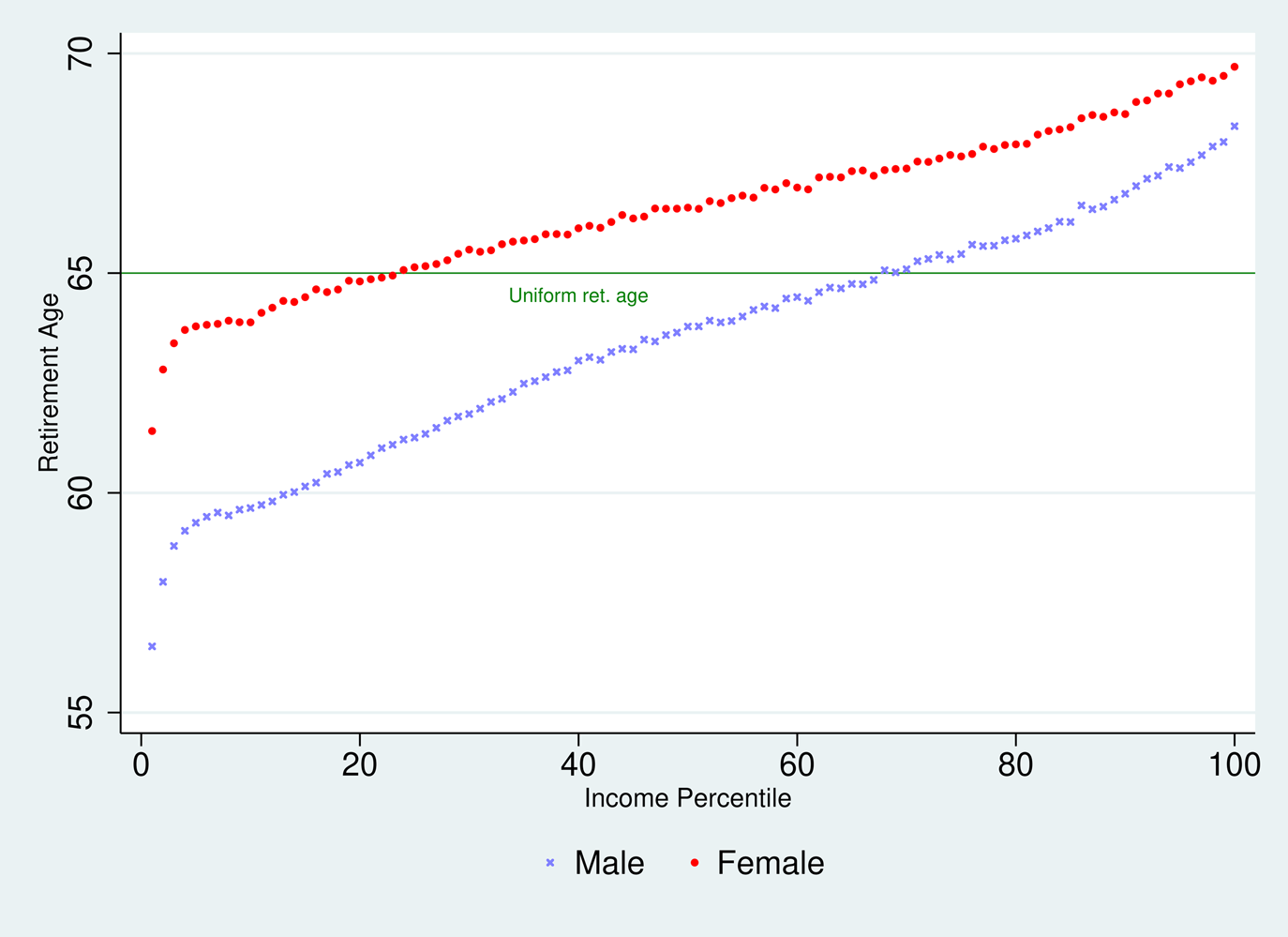
Figure 4. Beveridgian differentiated pension ages.
The key result is the one about the equity gains achieved via differentiation. It is reported on top of Table 1. We see values of 0.963 and 0.964 for (respectively) the Bismarckian and Beveridgian schemes. These are our best estimates of how much inequity indices can be brought down via retirement age differentiation. Remember that these indices are equal to (θ ′/θ); (b ′/b) as stated in Equations (15) and (19). Thus 1 − 0.963 or 1 − 0.964 tell us about the % reduction of pension instalmentFootnote 26 required to generate an equivalent gain in terms of pension fairness. We see it is relatively limited: less than 4% points of reduction of θ (Bismarck) or of the basic pension b (Beveridge) would be enough to generate the same equity gains as extensive retirement age differentiation across 200 gender × income categories; with retirement ages ranging from 56.5 to 69.7 (Bismarckian) or 54.2 to 71 (Beveridge) displayed in the lower part of Table 1. Also, one can get an idea of what the above results imply for the importance of the lump-sum paid upfront. Assuming that the (by 4%) reduced pension instalments are paid from the age of 65 to retirees with a 20-year life expectancy, following Equation (17), in a Beveridgian system, the lump-sum would represent approximately 0.004 × 20 × 12 = 9.6 month-equivalents of the current pension instalment. The calculus is less straightforward for Bismarckian system but results are similar.
Table 1. Numeric results: values of the equity gap indexa achieved via retirement age differentiation and the degree of de-annuitization needed to match these gains [without cohortal budget equivalenceb]
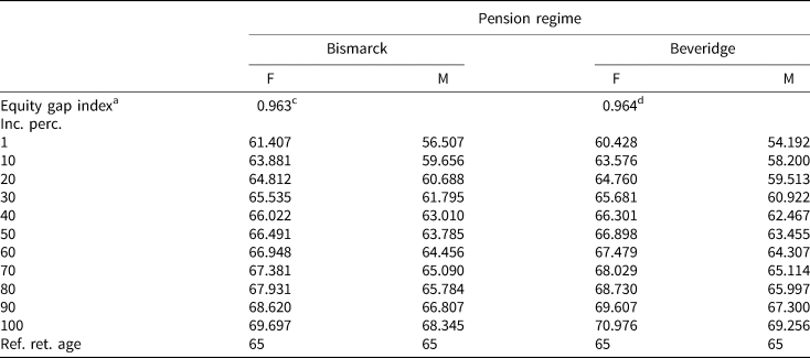
a The simulated values of equity gap indexes exposed in Equations (15) and (19). The propensity of these indices to be below 1 tells us simultaneously about (i) the equity gains that can be achieved via retirement age differentiation and (ii) the degree of de-annuitization required to generate an equivalent gain in terms of pension fairness. We report here the gains achieved by resorting to 200 different reference retirement ages/longevities (i.e., j = 1…200, corresponding to 2 genders × 100 income percentiles). The differentiated retirement ages we use are those visible in Figures 3 and 4. In the lower part of this table we report only a sample of them.
b Meaning that we assume that the planner ‘absorbs’ the net budgetary surplus(deficit) generated by the move from uniform to differentiated retirement age. Thus the move does not translate into higher(lower) value of θ and b to guarantee that the same total budget is spent on the cohort of pensioners.
c I Bismarck ∈ [0, 1] as defined by Equation (15).
d I Beveridge ∈ [0, 1] as defined by Equation (19).
4.3 Winners, losers
In this section, we explore the question of the support/opposition that partial de-annuitization might encounter. Our approach is quite simple. We consider that the support for de-annuitization depends on the share of short-lived individuals who get a higher lifetime actuarial fairness ratio (or benefits with a Beveridgian system). In Figure 5, it corresponds to all the individuals whose longevity is inferior to l*.
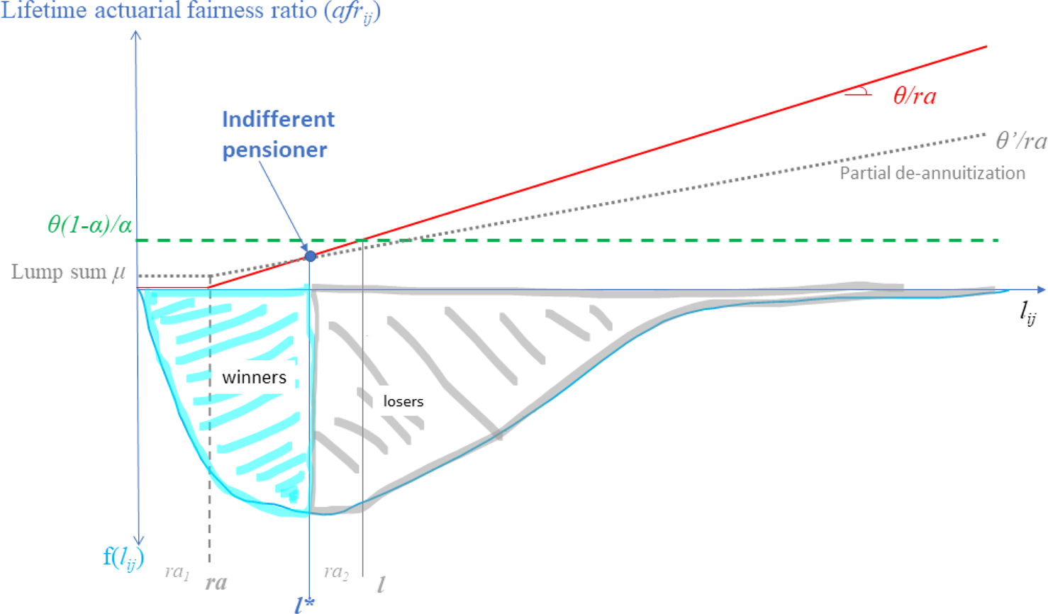
Figure 5. Partial de-annuitization: winners vs. losers.
Algebraically and numerically, one can show that the ‘indifferent’ pensioner is not influenced by the degree of de-annuitization. The point of indifference in Figure 5 and the corresponding longevity l* are fixed. Whatever the intensity of de-annuitization, there is always the same share of pensioners who gain from de-annuitization vs. uniform retirement age. Proof of this is in Appendix A4.Footnote 27
This said, it is important to stress that the value l* varies with the reference retirement age (ra). In Figure 6 we report simulation results on the share of (relatively short-lived) pensioners who would gain from de-annuitization. It is clearly a rising function of the reference retirement age. In policy terms this means that the support for de-annuitization is likely to rise the more policy makers increase the (unique) retirement age.
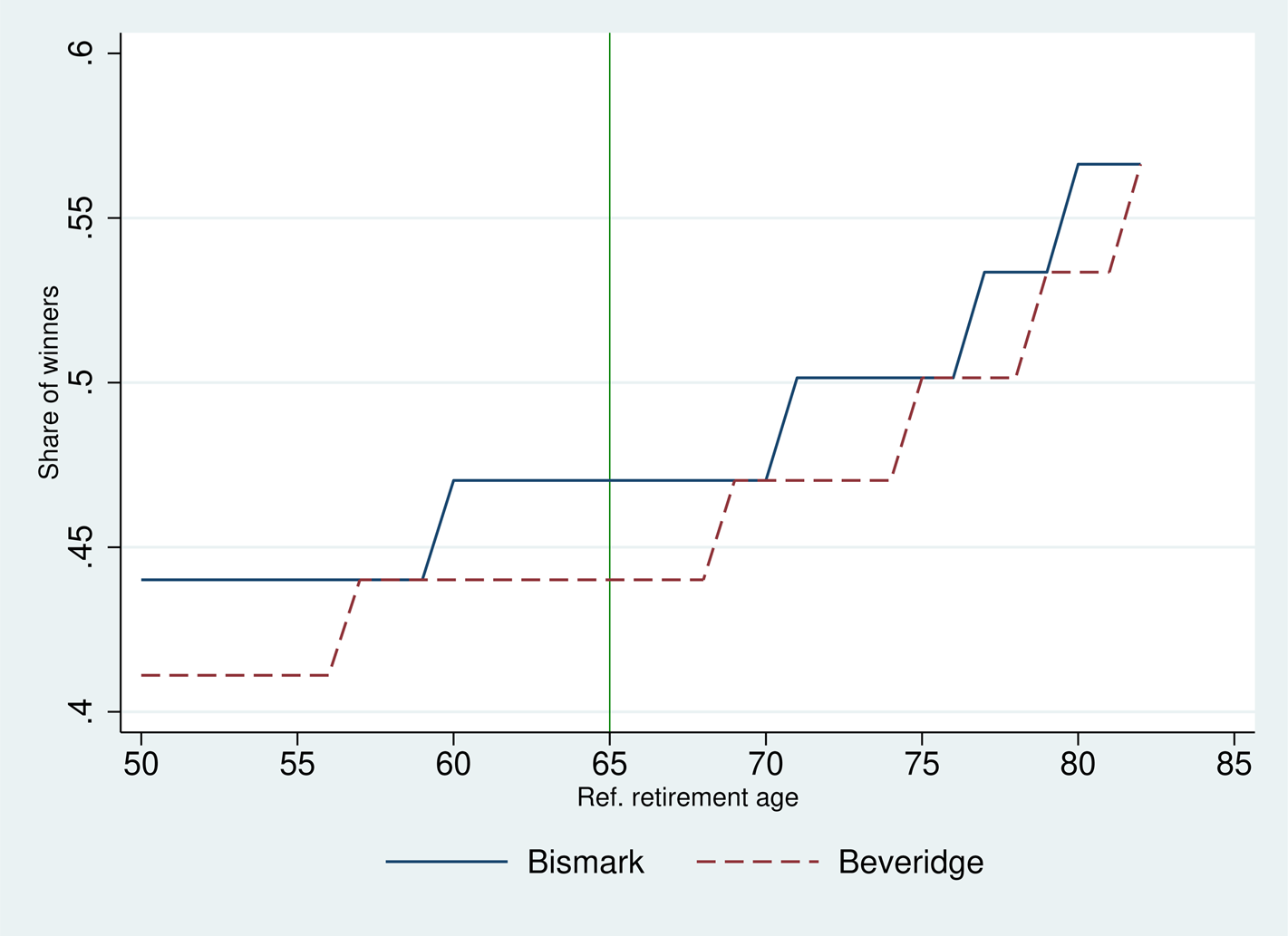
Figure 6. Partial de-annuitization: share of winners and ref. retirement age.
5. Context and policy feasibility
In the US context, and among economists who work on private/funded pensions, the dominant view is that people are ‘under-annuitized’ for their privately provided and funded pension. By that, our colleagues mean they are underinsured against the risk of outliving their pension capital (Yaari, Reference Yaari1965; Diamond and Mirrlees, Reference Diamond and Mirrlees1985; Diamond and Sheshinski, Reference Diamond and Sheshinski1995; Brown, Reference Brown2007). And one challenge is to understand the so-called annuity puzzle, i.e., the fact that annuities are rarely purchased (voluntarily) despite the longevity insurance they provide. One of the problem seems to be that people are too pessimistic about their longevity (O'Dea and Sturrock, Reference O'Dea and Sturrock2020; Benartzi et al., Reference Benartzi, Previtero and Thaler2021). A lot of recent effort has been made to understand the public's rejection of full-annuitization (Vidal-Meliá and Lejárraga-García, Reference Vidal-Meliá and Lejárraga-García2006; Clark et al., Reference Clark, Hammond and Vanderweide2019; Brown et al., Reference Brown, Kepteyn, Luttmer, Mitchell and Samek2021) and its preference for partial de-annuitization (Beshears et al., Reference Beshears, Choi, Laibson, Madrian and Zeldes2014; Dillingh and Zumbuehl, Reference Dillingh and Zumbuehl2021). These authors, for instance, find that allowing individuals to annuitize a fraction of their wealth increases their support for annuitization relative to a situation where annuitization is an ‘all or nothing’ decision.
The take-home message of this paper is also that pensions should be partially de-annuitized, even PAYG public ones. But the underlying context is quite different. In Europe and for public pensions organized on a PAYG basis, full and mandatory annuitization is the (unquestioned) rule. Also our key argument in favour of partial de-annuitization is not so much that the public prefers it, but that it is a simple and effective way of addressing the problem of the short-lived individuals. In contrast with the US/private and funded pension debate our starting point is not the risk of poverty at (very) old age but the risk of inequality inherent to full annuitization when the length of life varies a lot across individuals; what a burgeoning literature calls the risk of early death (Fleurbaey et al., Reference Fleurbaey, Leroux, Pestieau and Ponthière2016, Reference Fleurbaey, Leroux, Pestieau, Ponthière and Zuber2022; Leroux and Ponthiere, Reference Leroux and Ponthiere2018; Ponthiere, Reference Ponthiere2020).
The latter problem, and also evidence of a resurgent gap in life expectancy (Chetty et al., Reference Chetty, Stepner, Abraham, Lin, Scuderi, Turner, Bergeron and Cutler2016; Auerbach et al., Reference Auerbach, Charles, Coile, Gale, Goldman, Lee, Lucas and Orszag2017), is getting more and more attention among pension economists (Gustman and Steinmeier, Reference Gustman and Steinmeier2001; Bommier et al., Reference Bommier, Leroux and Lozachmeur2011; Haan et al., Reference Haan, Kemptner and Lüthen2019), but the focus is only on differentiation of treatment based on expected longevity differences across socio-demographic groups (Ayuso et al., Reference Ayuso, Bravo and Holzmann2016; Holzmann et al., Reference Holzmann, Alonso-García, Labit-Hardy and Villegas2017; Vandenberghe, Reference Vandenberghe2021) or occupations (Vermeer et al., Reference Vermeer, Mastrogiacomo and Van Soest2016). The parameters of differentiation investigated in that literature comprise the retirement age, and also the replacement rate or the contribution rate during the pension build-up phase (Bismarckian pensions), or simply the amount of the basic pension (Beveridgian pensions).
What we show in this paper is that partial de-annuitization of PAYG pensions would be as effective at addressing the inequalities and inefficiencies generated by longevity differences. And as far as we know this result is a novelty in the literature on pensions. If all (or most) longevity differences matter from a normative point of view,Footnote 28 for both the Bismarckian and Beverigdian versions of public PAGY pensions, we show that a modest de-annuitization – 4% point reduction of the monthly pension and the corresponding payment of an upfront lump sum – would be enough to match the equality gains recorded via extensive retirement differentiation.
Finally, the partial de-annuitization we propose here appears feasible from both a technical/financial and political point of view. First, being limited in magnitude it is unlikely to generate insurmountable liquidity and transition difficulties. We show that the lump-sums that would be paid correspond (on average) to less than one year of annuity payments (less than 12 monthly instalments). These sums could be borrowed from the market and financed by the savings corresponding to the stream of reduced monthly instalments. Also we do not a priori detect ‘cohabitation’ problems: older generations could stick to full annuitization, while the next ones would get partial de-annuitization. Second, partial de-annuitization as we model it in this paper is unlikely to significantly compromise the longevity insurance role of public pensions; the very one that pushes our US colleagues to recommend more annuitization, and correspond to the historical role of pensions that the general public probably still support to a large extent. Third, administratively, it is much less costly and easier to implement than retirement age differentiation.Footnote 29 It does not require upstream analysis of the determinants of longevity or the verification of pensioner's category as would, by definition, be the case with retirement age differentiation.Footnote 30 Fourth, unlike retirement age differentiation, de-annuitization is not prone to legal challenges. It amounts to treating everyone equally. By definition, this is not the case of differentiation. Would differentiating retirement age by gender be legal? Probably not in the US and in Europe. The European Court of justice bans any form of difference of treatment between women and men as to the legal age of retirement. Finally, it is also exempt of the risk of misreporting or moral hazard. De-annuitization amounts to paying a lump sum at a certain age to everyone. As shown repeatedly in public economics, these types of payments are exempt from risk of misreporting or disincentive to perform (here earn a lower wage conducive to a lower income percentile to get classified as a short-lived persons entitled to early retirement).
Acknowledgements
This research was financially supported by the convention ARC No 18-23-088. We would like to thank anonymous referees, UCLouvain colleagues and the audience of the SAS-Pension workshop for their helpful comments on earlier versions of this text.
Appendix A
A1 Graphical representation of Beveridge pensions
The first-best situation amounts to ensuring that every person receives the horizontal dashed line in terms of (lifetime) benefits ($b \kappa$![]() ) where κ is the number of years spent in retirement by the reference pensioner with longevity l. Actual/realized lifetime benefits correspond to the solid/doted rising lines. People who die before the retirement age receive no benefits. Beyond that point, lifetime benefits rise at a rate b.Footnote 31 Under uniform retirement age (solid rising line), only individuals whose longevity coincides with reference l get the first best. Under differentiated retirement age (doted rising lines, only two different retirement ages are depicted in Figure A1), the number of people who get on the green line a priori rises. But note again that situations synonymous with ‘undershooting’ or ‘overshooting’ are still very frequent.
) where κ is the number of years spent in retirement by the reference pensioner with longevity l. Actual/realized lifetime benefits correspond to the solid/doted rising lines. People who die before the retirement age receive no benefits. Beyond that point, lifetime benefits rise at a rate b.Footnote 31 Under uniform retirement age (solid rising line), only individuals whose longevity coincides with reference l get the first best. Under differentiated retirement age (doted rising lines, only two different retirement ages are depicted in Figure A1), the number of people who get on the green line a priori rises. But note again that situations synonymous with ‘undershooting’ or ‘overshooting’ are still very frequent.
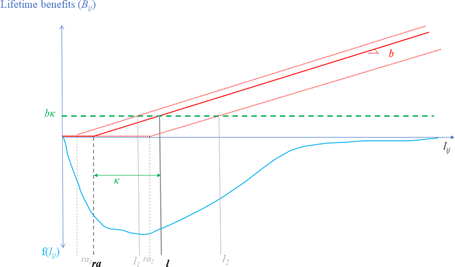
Figure A1. Beveridgian pension under uniform vs. diff. ret age.
A2 Cohortal budget equivalence under retirement age differentiation
Retirement age differentiation can generate budgetary savings in comparison with uniform retirement. This is because the overall (or average) time spent in retirement may go down. What is more, with a Bismarckian regime, the money not spent on those who live longer is likely to outweigh the cost of financing early retirement to the benefit of the short-lived individuals. If these budgetary savings are used to increase b (Beveridge) or θ (Bismarck) and so achieve cohortal budget equivalence, then the equity gaps (Equation (5)) – that inevitably still exist under retirement age differentiation – will be ‘priced’ at a higher rate. Say differently, in our (in)equity index, the time component of the gaps will be multiplied by a higher ‘price’ b (Beveridge) or θ (Bismarck). Thus the equity gains achieved in terms of years spent in retirement will be eroded by the (remaining) year gaps weighing more in monetary terms.
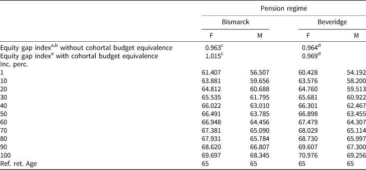
The algebra below identifies b (Beveridge) or θ (Bismarck) ensuring cohortal budget equivalence and discusses their determinants. But the key take-home result is visible in Table A1. The second line of the table reports the equity gains achieved by retirement age differentiation when cohortal budget equivalence is imposed. We see that, in particular for Bismarckian pensions, equity gains are lower and potentially negative, suggesting that the negative effect of higher ‘prices’ applicable to persistent gaps dominates the gains achieved by reducing the (time) magnitude of these gaps.
Table A1. Numeric results: values of the equity gap indexa achieved via retirement age differentiation (without and with cohortal budget equivalence)
Now we turn the algebra. To ensure strict budgetary equivalence, the Beveridgian planner should use an annuity b rad such that

The budget balancing b rad is thus inversely proportional to the change (possibly reduction) of aggregate time spent in retirement due to introducing different retirement ages.
The Bismarckian planner's equivalent problem is a bit more complex. She needs the ratio of benefits to contribution to be equivalent to what it is under uniform retirement. Formally we need
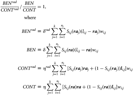
or equivalently
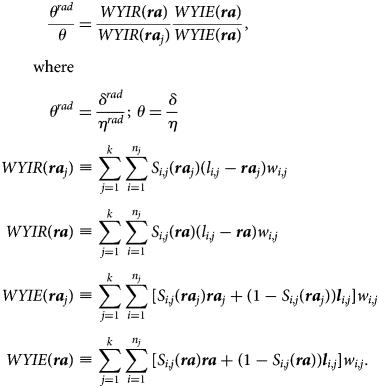
So θ rad should be inversely proportional to the change of the (wage-weighted)Footnote 32 years spent in retirement (WYIR(raj)) and proportional to the change in the (wage-weighted) years spent in employment (WYIE(raj)). If retirement age differentiation leads to fewer wage-weighted years spent in retirementFootnote 33 (fraction 1 to the rhs of Equation (A.3) is >1) and simultaneously more (wage-weighted) years spent working (fraction 2 >1) than the planner can finance θ rad > θ. This means that each years-in-retirement gap in Equation (6) are ‘priced’ at a higher rate, contributing to the erosion of the equity gains generated by retirement age differentiation.
A3 Cohortal budget equivalence under de-annuitization
Here, we identify the conditions for de-annuitization to generate, for a cohort, overall benefits matching what is spent under uniform retirement age.
We start with partial de-annuitization of Bismarckian pensions, where a uniform fraction ($\mu \equiv ( {LS_{i, j}/{\boldsymbol ra} \eta w_{i, j}} )$![]() ) of lifetime contributions (i.e., the ‘guaranteed’ part of the ratio) is handed over to every retiree. For a cohort, budget equivalence is achieved if the lump-sum payment LS i,j and the reduced annuity, calculated with a lower replacement rateδ ′, verify
) of lifetime contributions (i.e., the ‘guaranteed’ part of the ratio) is handed over to every retiree. For a cohort, budget equivalence is achieved if the lump-sum payment LS i,j and the reduced annuity, calculated with a lower replacement rateδ ′, verify
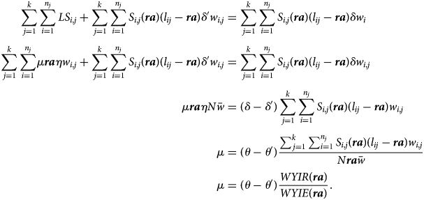
To move from line 2 to line 3, we regroup expressions with δ to the right-hand side. Considering that μ, ra, η are constant, we are left with $\mu {\boldsymbol ra} \eta \sum _{j = 1}^k \sum _{i = 1}^{n_j} w_{i, j}$![]() or equivalently $\mu {\boldsymbol ra} \eta N\bar{w}$
or equivalently $\mu {\boldsymbol ra} \eta N\bar{w}$![]() where Nis the size of the cohort and $\bar{w}$
where Nis the size of the cohort and $\bar{w}$![]() its average wage. On line 5 we have that WYIR(ra) is the overall (wage-weighted) number of years spent in retirement and WYIR(ra) is the overall (wage-weighted) number of years spent in employment.Footnote 34
its average wage. On line 5 we have that WYIR(ra) is the overall (wage-weighted) number of years spent in retirement and WYIR(ra) is the overall (wage-weighted) number of years spent in employment.Footnote 34
In a Beveridgian scheme, the uniform lump-sum payment LS and the reduced annuity b ′ must verify
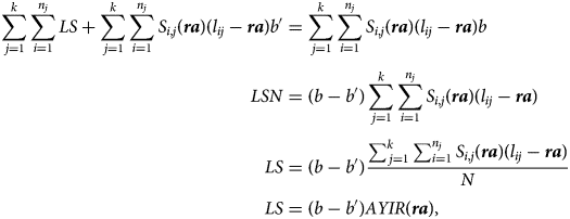
where AYIR(ra) is the average number of years spent in retirement.
A4 De-annuitization and the indifferent pensioner
Here we characterize algebraically the indifferent retiree (Figure 5). This is the person who is (or should be) indifferentFootnote 35 between what he gets under partial de-annuitization and under uniform retirement. With a Bismarckian system, that person has longevity l* such that
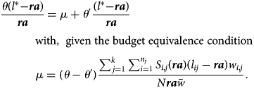
After some simple algebraic transformations we get

In other words, l* is independent of de-annuitization parameters μ and θ ′ < θ. So the intensity of de-annuitization has no impact on the longevity identifying the indifferent retiree. Note, however, that l* is a function of (uniform) retirement age (ra).
Similarly, with Beveridgian pension system, the indifferent pensioner has longevity l* that verifies

After some simple algebraic transformations we get

where, again, l* turns out to be independent of de-annuitization parameters LF and b ′ < b. So the intensity of de-annuitization has no impact on the longevity identifying the indifferent retiree. But note again that l* is a function of (uniform) retirement age (ra).

