


1. Introduction
This paper concerns the three-dimensional stationary incompressible Navier–Stokes equations
 \begin{equation} \left.
\begin{array}{@{}c@{}} \boldsymbol{v}\boldsymbol{\cdot}
\boldsymbol{\nabla} \boldsymbol{v} + p = \nu {\rm \Delta} \boldsymbol{v},\\
\boldsymbol{\nabla} \boldsymbol{\cdot}\boldsymbol{v} = 0,
\end{array}\right\}
\end{equation}
\begin{equation} \left.
\begin{array}{@{}c@{}} \boldsymbol{v}\boldsymbol{\cdot}
\boldsymbol{\nabla} \boldsymbol{v} + p = \nu {\rm \Delta} \boldsymbol{v},\\
\boldsymbol{\nabla} \boldsymbol{\cdot}\boldsymbol{v} = 0,
\end{array}\right\}
\end{equation}
where  $\boldsymbol{v} = \boldsymbol{v}(x) = (v_1(x),v_2(x),v_3(x))$ is the velocity vector,
  $p = p(x)$ denotes the scalar pressure and
  $\nu > 0$ is the viscosity constant. For the Navier–Stokes equations (1.1) in the whole space
  $\mathbb {R}^3$, it has been an open problem whether
  $\boldsymbol{v} \equiv 0$ is the only solution under the conditions that
  $\boldsymbol{v}$ has finite Dirichlet integral and vanishes at spatial infinity (see Galdi Reference Galdi2011, remark X.9.4). Seregin (Reference Seregin2018) reformulated the problem in such a way that any bounded solution
  $\boldsymbol{v}$ must be constant. There are many partial answers to this problem and, for instance, we refer readers to Carrillo, Pan & Zhang (Reference Carrillo, Pan and Zhang2020), Chae (Reference Chae2014), Chae & Wolf (Reference Chae and Wolf2016), Chamorro, Jarrín & Lemarié-Rieusset (Reference Chamorro, Jarrín and Lemarié-Rieusset2021), Koch et al. (Reference Koch, Nadirashvili, Seregin and Sverak2009) and Kozono, Terasawa & Wakasugi (Reference Kozono, Terasawa and Wakasugi2017) and references therein.
Recently, the Liouville-type theorems in non-compact domains in  $\mathbb {R}^3$ have also been studied. Carrillo et al. (Reference Carrillo, Pan, Zhang and Zhao2020) showed that a smooth solution with the finite Dirichlet integral to the Navier–Stokes equations (1.1) in a slab domain
  $\mathbb {R}^2 \times [0,1]$ with the no-slip boundary condition must be zero. Among other results, they also treated the axially symmetric case with the periodic boundary condition and proved the Liouville-type result under the finite Dirichlet integral. The assumption of the finite Dirichlet integral was relaxed by Tsai (Reference Tsai2021) and Bang et al. (Reference Bang, Gui, Wang and Xie2023). In particular, Bang et al. (Reference Bang, Gui, Wang and Xie2023) obtained the Liouville-type theorem on the Poiseuille flow of the Navier–Stokes equations (1.1) in a slab domain
  $\mathbb {R}^2 \times [0,1]$ with no-slip boundary condition. Indeed, they showed that if
  $(\boldsymbol{v},p)$ is a smooth solution satisfying
  $\| \boldsymbol{v} \|_{L^{\infty }} < {\rm \pi}$, then
  $\boldsymbol{v}$ must be the Poiseuille flow like
  $\boldsymbol{v} = (ax_3(1-x_3), bx_3(1-x_3), 0)$ with some constants
  $a,b \in \mathbb {R}$. Their result may be regarded as the generalized Liouville-type theorem on non-trivial flow.
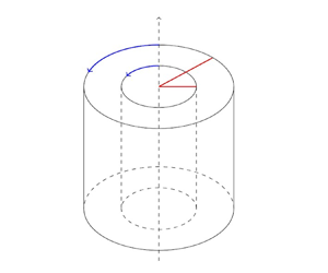
Motivated by these results, we have reached a natural question as to whether Liouville-type theorems hold for other non-trivial exact solutions of the Navier–Stokes equations. In this paper, we study the Liouville-type theorem on the Taylor–Couette–Poiseuille flow in a region between two rotating concentric cylinders. We also compare our mathematical uniqueness result with stability in the fluid mechanics in terms of Reynolds number and Taylor number in the case when the ratio of the radii of the two cylinders is sufficiently close to one.
1.1. Axially symmetric case
Let  $0 < R_1 < R_2$ be constants and let
  $\varOmega = \{ (x_1,x_2,x_3) \in \mathbb {R}^3 ; R_1 < \sqrt {x_1^2+x_2^2} < R_2 \}$, that is, a region between two concentric cylinders. In
  $\varOmega$, we consider the axially symmetric incompressible stationary Navier–Stokes equations in cylindrical coordinates:
 \begin{equation} \left.\begin{array}{@{}c@{}} \displaystyle ( v^r \partial_r + v^z \partial_z ) v^r - \dfrac{(v^{\theta})^2}{r} + \partial_r p =\nu \left( \partial_r^2 + \dfrac{1}{r} \partial_r + \partial_z^2 - \dfrac{1}{r^2} \right) v^r,\\ \displaystyle ( v^r \partial_r + v^z \partial_z ) v^{\theta} + \dfrac{v^r v^{\theta}}{r} =\nu \left( \partial_r^2 + \dfrac{1}{r} \partial_r + \partial_z^2 - \dfrac{1}{r^2} \right) v^{\theta},\\ \displaystyle ( v^r \partial_r + v^z \partial_z ) v^z + \partial_z p =\nu \left( \partial_r^2 + \dfrac{1}{r} \partial_r + \partial_z^2 \right) v^z,\\ \dfrac{1}{r} \partial_r (r v^r) + \partial_z v^z = 0, \end{array}\right\} \end{equation}
where  $r \in (R_1,R_2)$,
  $z \in \mathbb {R}$,
  $\boldsymbol{v} = \boldsymbol{v}(r,z) = v^r \boldsymbol {e}_r + v^{\theta } \boldsymbol {e}_{\theta } + v^z \boldsymbol {e}_z$ with
  $\boldsymbol {e}_r = (\cos \theta, \sin \theta, 0)$,
  $\boldsymbol {e}_{\theta } = (-\sin \theta, \cos \theta, 0)$,
  $\boldsymbol {e}_z = (0,0,1)$ denoting the basis of the cylindrical coordinate and
  $p = p(r,z)$. Moreover, we impose on
  $\boldsymbol{v}$ the boundary conditions
 \begin{equation} \left.\begin{array}{@{}c@{}} v^r(R_j,z) = v^z (R_j,z) = 0 \quad (j=1,2),\\ v^{\theta}(R_1,z) = R_1 \omega_1, \quad v^{\theta}(R_2,z) = R_2 \omega_2 , \end{array}\right\} \end{equation}
with some  $\omega _1, \omega _2 \in \mathbb {R}$, that is, the inner and outer cylinders rotate with angular velocities
  $\omega _1$ and
  $\omega _2$, respectively.
It is well known that there exists an exact solution to (1.2) called the Taylor–Couette flow:
 \begin{equation} \boldsymbol{v} = (0,v^{\theta},0) \quad \text{with } v^{\theta} =Ar + B\frac 1r, \end{equation}
where
 \begin{equation} A = \left\{ \begin{array}{@{}ll@{}} \displaystyle{ \dfrac{\mu - \eta^2}{1-\eta^2}\omega_1 }, & \omega_1 \ne 0, \\ \displaystyle{ \dfrac{1}{1-\eta^2}\omega_2 }, & \omega_1 = 0, \end{array}\right. \quad B = \left\{ \begin{array}{@{}ll@{}} \displaystyle{ \dfrac{1-\mu}{1-\eta^2}\omega_1 R_1^2 }, & \omega_1 \ne 0, \\ \displaystyle{ -\dfrac{1}{1-\eta^2}\omega_2 R_1^2 }, & \omega_1 = 0 , \end{array} \right. \end{equation}
with non-dimensional quantities  $\mu$ and
  $\eta$ given by
 \begin{equation} \mu = { \frac{\omega_2}{\omega_1} } \quad \mbox{for } \omega_1\ne 0, \quad \eta = { \frac{R_1}{R_2} }. \end{equation}
It is also known that the Taylor–Couette flow is stable if  $\omega _1$ is sufficiently small. However, if
  $\omega _1$ exceeds a certain critical value, then the Taylor–Couette flow becomes unstable and a fluid motion called the Taylor vortex appears (see e.g. Kirchgässner & Sorger Reference Kirchgässner and Sorger1969; Chossat & Iooss Reference Chossat and Iooss1994). For a recent result on the compressible fluid motion, we refer to Kagei & Teramoto (Reference Kagei and Teramoto2020).
In this paper, we show a Liouville-type theorem on the more generalized Taylor–Couette–Poiseuille flow including (1.4), provided that the velocity is not too large. Although the Taylor–Couette–Poiseuille flow below (equation (1.9)) is not altogether new (see e.g. Ma & Wang Reference Ma and Wang2009; Guy Raguin & Georgiadis Reference Guy Raguin and Georgiadis2024), our derivation itself seems to be new, because it is obtained from the fact that  $\partial _z \boldsymbol{v} \equiv 0$. The first main theorem reads as follows.
Theorem 1.1 Let  $(\boldsymbol{v},p)$ be an axially symmetric smooth solution of (1.2) in
  $\varOmega$ with the boundary conditions (1.3). There exists a constant
  $C_1(\nu,R_1,R_2)>0$ such that if
  $\omega _1, \omega _2$ and
  $\| \boldsymbol{v} \|_{L^{\infty }}$ satisfy
 \begin{equation} \max\{ R_1 |\omega_1|, R_2 |\omega_2| \} < C_1(\nu,R_1,R_2) \end{equation}
and
 \begin{equation} \| \boldsymbol{v} \|_{L^{\infty}(\varOmega)} < C_1(\nu,R_1,R_2), \end{equation}
respectively, then  $(\boldsymbol{v},p)$ must be the generalized Taylor–Couette–Poiseuille flow:
 \begin{equation} \left.\begin{array}{@{}c@{}} v^r\equiv0,\\ \displaystyle v^{\theta}=Ar + B\dfrac{1}{r},\\ \displaystyle v^z=\dfrac{a}{4\nu} R_{1}^{2} \left[ \left(\dfrac{r}{R_{1}}\right)^{2} - 1 + \dfrac{1-\eta^{2}}{\eta^{2}\log \eta} \log \left( \dfrac{r}{R_1} \right) \right],\\ \displaystyle p = az + b + \dfrac{A^2}{2} r^2 + 2AB \log r - \dfrac{B^2}{2}\dfrac {1}{r^2}, \end{array}\right\} \end{equation}
with some constants  $a, b \in \mathbb {R}$, where the constants
  $A$ and
  $B$ are the same as in ( 1.5 a,b). In particular, if the pressure
  $p$ is bounded or periodic in
  $z$, then the constant
  $a$ in (1.9) must be zero, and hence we have
  $v^z \equiv 0$, which means that
  $\boldsymbol{v}$ coincides with the well-known canonical Taylor–Couette flow given by (1.4).
Remark 1.1
(i) Since the boundary condition (1.3) implies
 $\max \{ R_1 |\omega _1|, R_2|\omega _2| \} \le \| \boldsymbol{v} \|_{L^{\infty }}$, the condition (1.7) is necessary for (1.8).
(ii) From the proof of theorem 1.1, we may take
$C_1(\nu,R_1,R_2)$ as
(1.10)where\begin{equation} C_1(\nu,R_1,R_2) = \frac{\nu}{2\sqrt{C_P}}, \end{equation}$C_P := {R_2(R_2-R_1)^2}/{R_1{\rm \pi} ^2}$ is related to the Poincaré inequality. This implies that if the viscosity $\nu$ is large in comparison with the radii $R_1$ and $R_2$, then the fluid motion remains as laminar flow, i.e. the generalized Taylor–Couette–Poiseuille flow (1.9). It should be noted that our assumptions (1.7) and (1.8) do not need to impose any smallness on the pressure $p$ of (1.2).(iii) Taylor (Reference Taylor1923) introduced a Taylor number
$Ta$ in a thin gap $\eta \approx 1$ defined by
(1.11)There is a critical value\begin{equation} Ta \equiv{-}\frac{2A\omega_1R_2^4}{\nu^2}(1-\eta)^4(1 + \mu). \end{equation}$Ta_{c}$ such that if $Ta < Ta_{c}$, then the Taylor–Couette flow (1.4) is stable. For simplicity, we consider the case when $\omega _2 =0$, i.e. $\mu =0$. Then it holds that
(1.12)By (1.7) and (1.10) we have\begin{equation} Ta = \frac{2}{\nu^2}\omega_1^2R_2^4 \frac{\eta^2}{1+\eta}(1-\eta)^3 = \frac{2}{\nu^2}R_2^2(R_1\omega_1)^2\frac{1}{1+\eta}(1-\eta)^3. \end{equation}(1.13)Hence it follows from theorem 1.1 that under hypotheses of (1.13) and (1.8), the Taylor–Couette–Poiseuille flow (1.9) is the unique solution of (1.2) with (1.3). On the other hand, Taylor (Reference Taylor1923) showed that\begin{equation} Ta < \frac{{\rm \pi}^2}{2}\frac{\eta}{1+\eta}(1-\eta). \end{equation}$Ta_c = 1708$, from which the Taylor–Couette flow (1.4) is stable under the condition that
(1.14)In comparison with (1.13) and (1.14), our uniqueness result seems to be quite restrictive from the viewpoint of the Taylor number\begin{equation} Ta < 1708. \end{equation}$Ta$. However, we should emphasize that uniqueness of solutions necessarily requires more restrictive conditions than those of stability.(iv) In the non-dimensional form of the (1.2), the Reynolds numbers
$Re_j$ are defined by
(1.15)Then, (1.10) implies that the assumption (1.7) is written as\begin{equation} Re_j = \frac{R_j\omega_j(R_2-R_1)}{\nu} \quad (j=1,2). \end{equation}(1.16)Namely, theorem 1.1 implies that if the Reynolds numbers of the inner and outer cylinders and the velocity are bounded by a certain constant determined only by means of radii\begin{equation} \max\{ Re_1, Re_2 \} < \frac{R_2-R_1}{\nu}C_1(\nu,R_1,R_2) = \frac{{\rm \pi} \sqrt{R_1}}{2\sqrt{R_2}} = \frac{\rm \pi}{2}\sqrt{\eta}. \end{equation}$R_1$ and $R_2$, then the axisymmetric flow must be necessarily the generalized Taylor–Couette–Poiseuille flow (1.9). Matsukawa & Tsukahara (Reference Matsukawa and Tsukahara2022) performed direct numerical simulation for $\eta = 0.833$, and showed that in the set $(Re_1, Re_2) = (400, -1000)$, the Taylor–Couette–Poiseuille flow becomes turbulent. For such an $\eta$, we have $\frac {{\rm \pi} }{2}\sqrt {\eta } = 1.476$ and, hence, under the hypothesis $\max \{ Re_1, Re_2 \} < 1.476$ with (1.8) the Taylor–Couette–Poiseuille flow (1.9) is the unique solution of (1.2) with (1.3). Since our result is on uniqueness of solutions, it may be reasonable that the Reynolds numbers are by far the smaller in comparison with occurrence of instability.(v) Kagei & Nishida (Reference Kagei and Nishida2015) and Kagei & Nishida (Reference Kagei and Nishida2019) investigated the plane Poiseuille flow for the compressible Navier–Stokes equations, and gave a mathematical proof of its instability for Reynolds numbers much less than the critical Reynolds number when the Mach number is suitably large.
(vi) The assumption that the pressure
$p$ is bounded or periodic in $z$ seems physically reasonable, and hence in a possible physical situation, the laminar axially symmetric flow $\boldsymbol{v}$ in the two rotating concentric cylinder is necessarily the canonical Taylor–Couette flow (1.4).(vii) Temam (Reference Temam1977, ch. II, § 4) studied the uniqueness and the non-uniqueness of the problem (1.2) in the case of
$\omega _2 = 0$ provided that the flow $\boldsymbol{v}$ of (1.2) is periodic in $z$. Introducing the disturbance $\boldsymbol{u}=(u^r, u^\theta, u^z)$ such that $\boldsymbol{v}$ has the form $\boldsymbol{v} = \boldsymbol{v}_0 + \boldsymbol{u}$ with $\boldsymbol{v}_0$ denoting the Taylor–Couette flow (1.4), he reduced such a question on uniqueness as to whether $\boldsymbol{u}\equiv 0$ in $\varOmega$. It was proved in Temam (Reference Temam1977, ch. II, proposition 4.2) that, under smallness hypotheses of the Reynolds number, $\boldsymbol{u} \equiv 0$ provided that $(u^r, u^z)$ is written by the stream function $\psi$ in the coordinate $(r, z)$ satisfying $\partial _r\psi (r_1, z)=\partial _r\psi (r_2, z)=0$. In comparison with Temam's result, we remove the assumption of periodicity in $z$ and avoid making use of such a stream function, although we impose on $\boldsymbol{v}$ the smallness condition (1.8).


1.2. General case
Next, we treat the general case in which axial symmetry is not necessarily assumed. Consider the same region  $\varOmega$ as in § 1.1, and the incompressible stationary Navier–Stokes equations in cylindrical coordinates in
  $\varOmega$:
 \begin{equation}
\left.\begin{array}{@{}c@{}} \displaystyle (
\boldsymbol{v}\boldsymbol{\cdot}\boldsymbol{\nabla} ) v^r -
\dfrac{(v^{\theta})^2}{r} + \partial_r p =\nu \left(
{\rm \Delta} - \dfrac{1}{r^2} \right) v^r - \nu \dfrac{2}{r^2}
\partial_{\theta} v^{\theta},\\
\displaystyle (\boldsymbol{v}\boldsymbol{\cdot}\boldsymbol{\nabla} )
v^{\theta} + \dfrac{v^r v^{\theta}}{r} + \dfrac{1}{r}
\partial_{\theta} p =\nu \left( {\rm \Delta} - \dfrac{1}{r^2}
\right) v^{\theta} + \nu \dfrac{2}{r^2}\partial_{\theta}
v^r,\\
\displaystyle (\boldsymbol{v}\boldsymbol{\cdot}\boldsymbol{\nabla} ) v^z +
\partial_z p=\nu {\rm \Delta} v^z,\\
\displaystyle \dfrac{1}{r} \partial_r (r v^r) +
\dfrac{1}{r} \partial_{\theta} v^{\theta} + \partial_z v^z=
0, \end{array}\right\}
\end{equation}
\begin{equation}
\left.\begin{array}{@{}c@{}} \displaystyle (
\boldsymbol{v}\boldsymbol{\cdot}\boldsymbol{\nabla} ) v^r -
\dfrac{(v^{\theta})^2}{r} + \partial_r p =\nu \left(
{\rm \Delta} - \dfrac{1}{r^2} \right) v^r - \nu \dfrac{2}{r^2}
\partial_{\theta} v^{\theta},\\
\displaystyle (\boldsymbol{v}\boldsymbol{\cdot}\boldsymbol{\nabla} )
v^{\theta} + \dfrac{v^r v^{\theta}}{r} + \dfrac{1}{r}
\partial_{\theta} p =\nu \left( {\rm \Delta} - \dfrac{1}{r^2}
\right) v^{\theta} + \nu \dfrac{2}{r^2}\partial_{\theta}
v^r,\\
\displaystyle (\boldsymbol{v}\boldsymbol{\cdot}\boldsymbol{\nabla} ) v^z +
\partial_z p=\nu {\rm \Delta} v^z,\\
\displaystyle \dfrac{1}{r} \partial_r (r v^r) +
\dfrac{1}{r} \partial_{\theta} v^{\theta} + \partial_z v^z=
0, \end{array}\right\}
\end{equation}where we have used the notations
 $$\begin{gather} (\boldsymbol{v}\boldsymbol{\cdot}\boldsymbol{\nabla} ) = v^r \partial_r + \frac{v^{\theta}}{r} \partial_{\theta} + v^z \partial_z, \end{gather}$$
 $$\begin{gather}\varDelta = \partial_r^2 + \frac{1}{r} \partial_r + \frac{1}{r^2} \partial_{\theta}^2 + \partial_z^2. \end{gather}$$
Moreover, we also impose on  $\boldsymbol{v}$ the same boundary conditions as (1.3), that is,
 \begin{equation} \left.\begin{array}{@{}c@{}} v^r(R_j,\theta,z) = v^z (R_j,\theta,z) = 0 \quad (j=1,2),\\ v^{\theta}(R_1,\theta,z) = R_1 \omega_1, \quad v^{\theta}(R_2,\theta,z) = R_2 \omega_2, \end{array}\right\} \end{equation}
with some  $\omega _{1}, \omega _{2} \in \mathbb {R}$.
For the general case, under similar assumptions to (1.7) and (1.8), we have the following Liouville-type theorem for  $(\partial _{\theta }\boldsymbol{v},\partial _{\theta }p)$ which shows axial symmetry of the solutions to (1.17).
Theorem 1.2 Let  $(\boldsymbol{v},p)$ be a smooth solution of (1.17) in
  $\varOmega$ with the boundary conditions (1.20). There exists a constant
  $C_2(\nu,R_1,R_2)>0$ such that if
  $\omega _1, \omega _2$ and
  $\| \boldsymbol{v} \|_{L^{\infty }}$ satisfy
 \begin{equation} \max\{ R_1 |\omega_1|, R_2 |\omega_2| \} < C_2(\nu,R_1,R_2) \end{equation}
and
 \begin{equation} \| \boldsymbol{v} \|_{L^{\infty}(\varOmega)} < C_2(\nu,R_1,R_2), \end{equation}
respectively, then it holds that  $\partial _{\theta }\boldsymbol{v} \equiv 0$ and
  $\partial _{\theta }p \equiv 0$ in
  $\varOmega$, that is,
  $(\boldsymbol{v},p)$ is axially symmetric.
Remark 1.2 From the proof of theorem 1.2, we may take the constant  $C_2(\nu, R_1, R_2)$ as
 \begin{equation} C_2(\nu, R_1, R_2) = \nu \left( \sqrt{C_P} \left( 2 + \frac{C_P}{R_1^2} \right) + \frac{3C_P}{2R_1} \right)^{{-}1}, \end{equation}
where  $C_P := {R_2(R_2-R_1)^2}/{R_1{\rm \pi} ^2}$. We should emphasize that any assumption on smallness of the pressure
  $p$ of (1.17) is redundant.
Combining theorems 1.1 and 1.2, we immediately reach the following Liouville-type theorem for the general case.
Corollary 1.3 Let  $(\boldsymbol{v},p)$ be a smooth solution of (1.17) in
  $\varOmega$ with the boundary conditions (1.20). Let
  $C_1(\nu,R_1,R_2)$ and
  $C_2(\nu,R_1,R_2)$ be the same constants as in theorems 1.1 and 1.2, respectively. We set
  $C_\ast (\nu,R_1,R_2) \equiv \min \{ C_1(\nu,R_1,R_2), C_2(\nu,R_1,R_2) \}$. Suppose that
  $(\boldsymbol{v},p)$ is a smooth solution of (1.17) in
  $\varOmega$ with the boundary conditions (1.20). If
  $\omega _1, \omega _2$ and
  $\boldsymbol{v}$ satisfy
 \begin{equation} \max\{ R_1 |\omega_1|, R_2 |\omega_2| \} < C_\ast(\nu,R_1,R_2) \end{equation}
and
 \begin{equation} \| \boldsymbol{v} \|_{L^{\infty}(\varOmega)} < C_\ast(\nu,R_1,R_2), \end{equation}
respectively, then  $(\boldsymbol{v},p)$ is axially symmetric and coincides with the generalized Taylor–Couette–Poiseuille flow given by (1.9). In particular, if
  $p$ is bounded or periodic in
  $z$, then
  $\boldsymbol{v}$ is necessarily the canonical Taylor–Couette flow (1.4).
Remark 1.3 It is easy to see that the generalized Taylor–Couette–Poiseuille flow (1.9) is also a solution of the Stokes equations in  $\varOmega$ with the same boundary condition (1.3). Hence without any assumption on smallness of
  $\|\boldsymbol{v}\|_{L^\infty (\varOmega )}$ as in (1.7) it holds that any bounded smooth solution
  $\boldsymbol{v}$ of the Stokes equations uniquely coincides with the generalized Taylor–Couette–Poiseuille flow (1.9) . In particular, if the pressure
  $p$ is bounded or periodic in
  $z$, then
  $\boldsymbol{v}$ is necessarily the canonical Taylor–Couette flow (1.4). This may be regarded as the Liouville-type theorem on the Stokes equations.
2. Preliminaries
In what follows,  $C$ denotes generic constants which may change from line to line. Also, the operators
  $\nabla _{r,z}$ and
  $\nabla _{r,\theta,z}$ stand for
  $\nabla _{r,z}\, f(r,z) = (\partial _r\, f, \partial _z\, f)(r,z)$ and
  $\nabla _{r,\theta,z}\,f(r,\theta,z) = (\partial _r f, \partial _{\theta } f, \partial _z\, f)(r,\theta,z)$, respectively.
We first state the boundedness of derivatives of solutions. This can be proved in the same way as in Bang et al. (Reference Bang, Gui, Wang and Xie2023, lemma 2.3) in which the three-dimensional slab domain is treated, since all estimates in the proof are local and do not depend on the shape of  $\varOmega$.
Lemma 2.1 Let  $(\boldsymbol{v},p)$ be a smooth solution of the Navier–Stokes equations (1.1) in
  $\varOmega$ with the boundary conditions (1.3). Assume that
  $v$ is bounded. Then,
  $\nabla _{r,\theta,z} \boldsymbol{v}, \nabla _{r,\theta,z}^2 \boldsymbol{v}$ and
  $\nabla _{r,\theta,z}p$ are also bounded.
Next, we prepare the test function used in this paper. Let  $L>1$ and define
 \begin{equation} \varphi_L(z) = \begin{cases} 1 & (|z| < L-1),\\ L-|z| & (L-1 \le |z| \le L),\\ 0 & (|z| > L). \end{cases} \end{equation}
Also, we put
 \begin{equation} \varSigma_L = \{ x \in \varOmega \mid L-1 \le |z| \le L\}. \end{equation}
Note that  $\textrm {supp} \partial _z \varphi _L \subset \varSigma _L$.
Finally, we prove a Poincaré-type inequality for the  $r$ direction in
  $\varOmega$ and
  $\varSigma _L$, which will be used for
  $\partial _z \boldsymbol{v}$ and
  $\partial _{\theta } \boldsymbol{v}$.
Lemma 2.2 Let  $f = f(r,\theta,z)$ be a smooth function on
  $\bar {\varOmega }$ satisfying the boundary condition
  $f(R_j, \theta, z) = 0$ (
 $\,j=1,2$). Let
  $L > 1$. Then, we have
 \begin{equation} \|\, f \sqrt{\varphi_L} \|_{L^2(D)} \le \sqrt{C_P} \| \partial_r f \sqrt{\varphi_L} \|_{L^2(D)}, \end{equation}
where  $D$ denotes
  $\varOmega$ or
  $\varSigma _L$ and
 \begin{equation} C_P = \frac{R_2(R_2-R_1)^2}{R_1 {\rm \pi}^2}. \end{equation}
Proof. When  $D = \varOmega$, using cylindrical coordinates and applying the Poincaré inequality in the
  $r$ direction, we calculate
 \begin{align} \|\, f \sqrt{\varphi_L} \|_{L^2(\varOmega)}^2 &=\int_{\mathbb{R}} \int_0^{2{\rm \pi}} \|\, f \sqrt{r} \|_{L^2(R_1,R_2)}^2 \varphi_L(z) \,{\rm d} \theta \, {\rm d} z \nonumber\\ &\le R_2 \int_{\mathbb{R}} \int_0^{2{\rm \pi}} \|\, f \|_{L^2(R_1,R_2)}^2 \varphi_L(z) \,{\rm d} \theta \, {\rm d} z \nonumber\\ &\le R_2 \frac{(R_2-R_1)^2}{{\rm \pi}^2} \int_{\mathbb{R}} \int_0^{2{\rm \pi}} \| \partial_r f\|_{L^2(R_1,R_2)}^2 \varphi_L(z) \,{\rm d} \theta \, {\rm d} z \nonumber\\ &\le \frac{R_2(R_2-R_1)^2}{R_1 {\rm \pi}^2} \int_{\mathbb{R}} \int_0^{2{\rm \pi}} \| \partial_r f \sqrt{r} \|_{L^2(R_1,R_2)}^2 \varphi_L(z) \,{\rm d} \theta \, {\rm d} z \nonumber\\ &=C_P\| \partial_r f \sqrt{\varphi_L} \|_{L^2(\varOmega)}^2. \end{align}
The case  $D = \varSigma _L$ can be proved in completely the same way.
3. Proof of theorem 1.1
Let us prove theorem 1.1. Assume that  $(\boldsymbol{v},p)$ is an axially symmetric smooth solution of (1.2) in
  $\varOmega$. Following the argument of Bang et al. (Reference Bang, Gui, Wang and Xie2023), we first show
 \begin{equation} \partial_z \boldsymbol{v} \equiv 0. \end{equation}
To this end, we differentiate (1.2) with respect to  $z$ and obtain
 \begin{equation}
\left.\begin{array}{@{}l@{}} ( \partial_z v^r \partial_r +
\partial_z v^z \partial_z ) v^r + ( v^r \partial_r + v^z
\partial_z ) \partial_z v^r - \dfrac{2v^{\theta} \partial_z
v^{\theta}}{r} + \partial_z \partial_r p\\
\qquad\qquad =\nu \left(
\partial_r^2 + \dfrac{1}{r} \partial_r + \partial_z^2 -
\dfrac{1}{r^2} \right) \partial_z v^r,\\
( \partial_z v^r \partial_r + \partial_z v^z \partial_z ) v^{\theta} + ( v^r
\partial_r + v^z \partial_z ) \partial_z v^{\theta} +
\dfrac{v^{\theta} \partial_z v^r + v^r \partial_z
v^{\theta} }{r}\\
\qquad\qquad =\nu \left( \partial_r^2 + \dfrac{1}{r}
\partial_r + \partial_z^2 - \dfrac{1}{r^2} \right)
\partial_z v^{\theta},\\
( \partial_z v^r \partial_r +
\partial_z v^z \partial_z ) v^z + ( v^r \partial_r + v^z
\partial_z ) \partial_z v^z + \partial_z^2 p= \nu \left(
\partial_r^2 + \dfrac{1}{r} \partial_r + \partial_z^2
\right) \partial_z v^z,\\
\qquad\qquad\qquad\qquad \qquad\partial_z \partial_r v^r +
\dfrac{\partial_z v^r}{r} + \partial_z^2 v^z = 0.
\end{array}\right\}
\end{equation}
\begin{equation}
\left.\begin{array}{@{}l@{}} ( \partial_z v^r \partial_r +
\partial_z v^z \partial_z ) v^r + ( v^r \partial_r + v^z
\partial_z ) \partial_z v^r - \dfrac{2v^{\theta} \partial_z
v^{\theta}}{r} + \partial_z \partial_r p\\
\qquad\qquad =\nu \left(
\partial_r^2 + \dfrac{1}{r} \partial_r + \partial_z^2 -
\dfrac{1}{r^2} \right) \partial_z v^r,\\
( \partial_z v^r \partial_r + \partial_z v^z \partial_z ) v^{\theta} + ( v^r
\partial_r + v^z \partial_z ) \partial_z v^{\theta} +
\dfrac{v^{\theta} \partial_z v^r + v^r \partial_z
v^{\theta} }{r}\\
\qquad\qquad =\nu \left( \partial_r^2 + \dfrac{1}{r}
\partial_r + \partial_z^2 - \dfrac{1}{r^2} \right)
\partial_z v^{\theta},\\
( \partial_z v^r \partial_r +
\partial_z v^z \partial_z ) v^z + ( v^r \partial_r + v^z
\partial_z ) \partial_z v^z + \partial_z^2 p= \nu \left(
\partial_r^2 + \dfrac{1}{r} \partial_r + \partial_z^2
\right) \partial_z v^z,\\
\qquad\qquad\qquad\qquad \qquad\partial_z \partial_r v^r +
\dfrac{\partial_z v^r}{r} + \partial_z^2 v^z = 0.
\end{array}\right\}
\end{equation}
Moreover, we have the boundary conditions for  $\partial _z v$:
 \begin{equation} \partial_z v (R_j, z) = 0 \quad (j=1,2). \end{equation}
Let  $L > 1$ and take the test function
  $\varphi _L$ and the region
  $\varSigma _L$ defined by (2.1) and (2.2), respectively. We multiply the equations of
  $v^r, v^{\theta }, v^z$ in (3.2) by
  $\partial _z v^r \varphi _L(z)$,
  $\partial _z v^{\theta } \varphi _L(z)$,
  $\partial _z v^z \varphi _L(z)$, respectively, and sum them and integrate them over
  $\varOmega$. Then, we have the integral identity
 \begin{equation} I = II + III + IV + V. \end{equation}
Here,  $I = I^r + I^{\theta } + I^z$ is the sum related to the viscous terms of the right-hand side of (3.2) defined by
 $$\begin{gather} I^{\lambda} =\nu \int_{\varOmega} \left( \partial_r^2 + \frac{1}{r} \partial_r + \partial_z^2 - \frac{1}{r^2} \right) \partial_z v^{\lambda} \partial_z v^{\lambda} \varphi_L(z) \,{{\rm d}\kern 0.06em x}\quad (\lambda = r,\theta), \end{gather}$$
 $$\begin{gather}I^z=\nu \int_{\varOmega} \left( \partial_r^2 + \frac{1}{r} \partial_r + \partial_z^2 \right) \partial_z v^{z} \partial_z v^z \varphi_L(z) \,{{\rm d}\kern 0.06em x}. \end{gather}$$
Terms  $II$,
$II$,  $III$ and
  $IV$ are related to the nonlinear terms of the left-hand side of (3.2) defined by
 \begin{align} II&= \sum_{\lambda=r,\theta,z} II^{\lambda} = \sum_{\lambda=r,\theta,z} \int_{\varOmega} \left( \partial_z v^r \partial_r + \partial_z v^z \partial_z \right) v^{\lambda} \partial_z v^{\lambda} \varphi_L(z) \,{{\rm d}\kern 0.06em x}, \end{align}
 \begin{align} III&= \sum_{\lambda=r,\theta,z} III^{\lambda} =\sum_{\lambda=r,\theta,z} \int_{\varOmega} \left( v^r \partial_r + v^z \partial_z \right) \partial_z v^{\lambda} \partial_z v^{\lambda} \varphi_L(z) \,{{\rm d}\kern 0.06em x}, \end{align}
 \begin{align} IV&={-}2 \int_{\varOmega} \frac{v^{\theta} \partial_z v^{\theta}}{r} \partial_z v^r \varphi_L(z) \,{{\rm d}\kern 0.06em x} + \int_{\varOmega} \frac{v^{\theta} \partial_z v^r + v^r \partial_z v^{\theta} }{r} \partial_z v^{\theta} \varphi_L(z) \,{{\rm d}\kern 0.06em x} \nonumber\\&= \int_{\varOmega} \frac{1}{r} \left( v^r \partial_z v^{\theta} - v^{\theta} \partial_z v^r \right) \partial_z v^{\theta} \varphi_L(z) \,{{\rm d}\kern 0.06em x}, \end{align}
respectively. Finally, term  $V$ is the sum related to the pressure terms of (3.2) defined by
 \begin{equation} V = \int_{\varOmega} ( \partial_z\partial_r p \partial_z v^r + \partial_z^2 p \partial_z v^z ) \varphi_L(z) \,{{\rm d}\kern 0.06em x}. \end{equation}
First, we compute the viscous terms  $I$. For
  $\lambda = r, \theta$, integration by parts with noting that
  $r(\partial _r^2 + ({1}/{r})\partial _r) = \partial _r (r \partial _r)$ implies
 \begin{align} I^{\lambda}&= \nu \int_{\varOmega} \left( \partial_r^2 + \frac{1}{r} \partial_r + \partial_z^2 - \frac{1}{r^2} \right) \partial_z v^{\lambda} \partial_z v^{\lambda} \varphi_L(z) \,{{\rm d}\kern 0.06em x} \nonumber\\ &={-} 2{\rm \pi} \nu \int_{\mathbb{R}} \int_{R_1}^{R_2} \left(|\partial_r \partial_z v^{\lambda} |^2 + | \partial_z^2 v^{\lambda} |^2 + \frac{|\partial_z v^{\lambda}|^2}{r^2} \right) \varphi_L(z) r \,{\rm d} r\, {\rm d} z \nonumber\\ &\quad- 2{\rm \pi} \nu \int_{\mathbb{R}} \int_{R_1}^{R_2} \partial_z^2 v^{\lambda} \partial_z v^{\lambda} \partial_z \varphi_L(z) r \,{\rm d} r\, {\rm d} z \nonumber\\ &=: I_1^{\lambda} + I_2^{\lambda}. \end{align}
In the same way, for  $I^z$, we have
 \begin{align} I^z&=\nu \int_{\varOmega} \left( \partial_r^2 + \frac{1}{r} \partial_r + \partial_z^2 \right) \partial_z v^{z} \partial_z v^z \varphi_L(z) \,{{\rm d}\kern 0.06em x} \nonumber\\ &={-} 2{\rm \pi} \nu \int_{\mathbb{R}} \int_{R_1}^{R_2} (|\partial_r \partial_z v^{z} |^2 + | \partial_z^2 v^{z} |^2 ) \varphi_L(z) r\,{\rm d} r\, {\rm d} z \nonumber\\ &\quad- 2{\rm \pi} \nu \int_{\mathbb{R}} \int_{R_1}^{R_2} \partial_z^2 v^{z} \partial_z v^{z} \partial_z \varphi_L(z) r \,{\rm d} r\, {\rm d} z \nonumber\\ &=: I_1^z + I_2^z. \end{align}
Now, for a later purpose, we express the sum of good terms by  $Y(L)$:
 \begin{align} Y(L)&:={-} (I_1^{r} + I_1^{\theta} + I_1^z) \nonumber\\ &=\nu \left( \| \partial_r \partial_z \boldsymbol{v} \sqrt{\varphi_L} \|_{L^2(\varOmega)}^2 + \| \partial_z^2 \boldsymbol{v} \sqrt{\varphi_L} \|_{L^2(\varOmega)}^2 + \sum_{\lambda=r,\theta} \| r^{{-}1} \partial_z v^{\lambda} \sqrt{\varphi_L} \|_{L^2(\varOmega)}^2 \right). \end{align}
We remark that the definition of  $\varphi _L(z)$ (see (2.1)) implies
 \begin{equation} Y'(L)=\nu \left( \| \partial_r \partial_z \boldsymbol{v} \|_{L^2(\varSigma_L)}^2 + \| \partial_z^2 \boldsymbol{v} \|_{L^2(\varSigma_L)}^2 + \sum_{\lambda=r,\theta} \| r^{{-}1} \partial_z v^{\lambda} \|_{L^2(\varSigma_L)}^2 \right). \end{equation}
By using this  $Y(L)$, term
  $I$ can be written as
 \begin{equation} I ={-} Y(L) + \sum_{\lambda=r,\theta,z} I_2^{\lambda}. \end{equation}
Let us estimate the remainder terms  $I_2^{\lambda }$ for
  $\lambda = r,\theta,z$. Since
  $\partial _z v^{\lambda } \in L^{\infty }(\varOmega )$ by lemma 2.1 and
  $|\varSigma _L| \le C$ with some constant
  $C$ independent of
  $L$, we estimate
 \begin{equation} |I_2^{\lambda}| \le C \| \partial_z^2 v^{\lambda} \|_{L^2(\varSigma_L)} \| \partial_z v^{\lambda} \|_{L^2(\varSigma_L)} \le C \| \partial_z^2 \boldsymbol{v} \|_{L^2(\varSigma_L)} \le C \sqrt{Y'(L)}, \end{equation}
where the constant  $C$ is independent of
  $L$.
$L$.
Next, we consider the nonlinear term  $II$. By integration by parts and the divergence-free condition
  $\partial _r (r \partial _z v^r) + \partial _z (r \partial _z v^z) = 0$, terms
  $II^{\lambda }$ for
  $\lambda = r,\theta,z$ are written as
 \begin{align} II^{\lambda} &={-} 2{\rm \pi} \int_{\mathbb{R}} \int_{R_1}^{R_2} (\partial_z v^r \partial_r + \partial_z v^{z} \partial_z ) \partial_z v^{\lambda} v^{\lambda} \varphi_L(z) r \,{\rm d} r\, {\rm d} z \nonumber\\ &\quad - 2{\rm \pi}\int_{\mathbb{R}} \int_{R_1}^{R_2} \partial_z v^{z} v^{\lambda} \partial_z v^{\lambda } \partial_z \varphi_L(z) r \,{\rm d} r\, {\rm d} z \nonumber\\ &=: II_1^{\lambda} + II_2^{\lambda}. \end{align}
The Hölder inequality implies
 \begin{align} |II^{\lambda}_{1}| &\le\| \partial_z v^r \sqrt{\varphi_L} \|_{L^2(\varOmega)} \| \partial_r \partial_z v^{\lambda} \sqrt{\varphi_L} \|_{L^2(\varOmega)} \| \boldsymbol{v} \|_{L^{\infty}(\varOmega)} \nonumber\\ &\quad + \| \partial_z v^z \sqrt{\varphi_L} \|_{L^2(\varOmega)} \| \partial_z^2 v^{\lambda} \sqrt{\varphi_L} \|_{L^2(\varOmega)} \| \boldsymbol{v} \|_{L^{\infty}(\varOmega)}. \end{align}
Moreover, by noting the boundary condition (3.3) and applying lemma 2.2, we further estimate
 \begin{align} |II_1^{\lambda}| &\le \| \boldsymbol{v} \|_{L^{\infty}(\varOmega)} \sqrt{C_P} ( \| \partial_r \partial_z v^r \sqrt{\varphi_L} \|_{L^2(\varOmega)} \| \partial_r \partial_z v^{\lambda} \sqrt{\varphi_L} \|_{L^2(\varOmega)}\nonumber\\ &\quad+ \| \partial_r\partial_z v^z \sqrt{\varphi_L} \|_{L^2(\varOmega)} \| \partial_z^2 v^{\lambda} \sqrt{\varphi_L} \|_{L^2(\varOmega)}). \end{align}
Hence, to term  $II_1 := II_1^{r} + II_1^{\theta } + II_1^z$, we apply the Schwarz inequality to conclude
 \begin{align} |II_1| &\le \| \boldsymbol{v} \|_{L^{\infty}(\varOmega)} \sqrt{C_P} \left( 2 \| \partial_r \partial_z v^r \sqrt{\varphi_L} \|_{L^2(\varOmega)}^2 + \frac{1}{2} \sum_{\lambda=r,\theta,z} \| \partial_r\partial_z v^{\lambda} \sqrt{\varphi_L} \|_{L^2(\varOmega)}^2 \right. \nonumber\\ & \quad +\left. 2 \| \partial_r \partial_z v^z \sqrt{\varphi_L} \|_{L^2(\varOmega)}^2 + \frac{1}{2} \sum_{\lambda=r,\theta,z} \| \partial_z^2 v^{\lambda} \sqrt{\varphi_L} \|_{L^2(\varOmega)}^2 \right). \end{align}
Note that the terms in parentheses are members of  $Y(L)$. Similarly to (3.16) we have by lemma 2.1 that
 \begin{equation} \|\partial_z\boldsymbol{v}\|_{L^2(\varSigma_L)} \le \|\partial_z\boldsymbol{v}\|_{L^\infty(\varOmega)}|\varSigma_L|^{1/2} \le C, \end{equation}
with the constant  $C$ independent of
  $L$. Hence, applying the Poincáre inequality in
  $\varSigma _L$ with the aid of (3.3) to the estimate for term
  $II_2 := II_2^r + II_2^{\theta } + II_2^z$, we have by the Hölder inequality that
 \begin{equation} |II_2| \le C \| \partial_z \boldsymbol{v} \|_{L^2(\varSigma_L)}^2 \| \boldsymbol{v} \|_{L^{\infty}(\varOmega)} \le C \| \partial_r \partial_z \boldsymbol{v} \|_{L^{2}(\varSigma_L)} \le C\sqrt{Y'(L)}. \end{equation}
 Let us estimate term  $III$. For
  $\lambda = r, \theta, z$, we write
  $III^{\lambda }$ as
 \begin{equation} III^{\lambda} = 2{\rm \pi} \int_{\mathbb{R}} \int_{R_1}^{R_2} ( v^r \partial_r + v^z \partial_z ) \left( \frac{1}{2} |\partial_z v^{\lambda} |^2 \right) \varphi_L(z) r \,{\rm d} r\, {\rm d} z. \end{equation}
Since the divergence-free condition means that  $\partial _r (r v^r) + \partial _z (r v^z) = 0$, we have by integration by parts with the aid of (3.3) that
 \begin{equation} III^{\lambda} ={-} {\rm \pi}\int_{\mathbb{R}} \int_{R_1}^{R_2} v^z \partial_z \varphi_L(z) |\partial_z v^{\lambda} |^2 r \,{\rm d} r\, {\rm d} z. \end{equation}
Then, in the same way as for term  $II_2$, we obtain
 \begin{equation} |III| \le C \| \partial_r \partial_z \boldsymbol{v} \|_{L^{2}(\varSigma_L)} \le C \sqrt{Y'(L)}. \end{equation}
 The remaining nonlinear term  $IV$ can be treated similarly to
  $I$. Indeed, using the Hölder inequality and lemma 2.2, we have
 \begin{align} |IV| &\le \| r^{{-}1}
\partial_z v^{r} \sqrt{\varphi_L} \|_{L^2(\varOmega)} \|
\partial_z v^{\theta} \sqrt{\varphi_L} \|_{L^2(\varOmega)}
\| \boldsymbol{v} \|_{L^{\infty}(\varOmega)} \nonumber\\
&\quad+ \| r^{{-}1} \partial_z v^{\theta} \sqrt{\varphi_L}
\|_{L^2(\varOmega)} \| \partial_z v^{\theta}
\sqrt{\varphi_L} \|_{L^2(\varOmega)} \| \boldsymbol{v}
\|_{L^{\infty}(\varOmega)} \nonumber\\
&\le\| \boldsymbol{v} \|_{L^{\infty}(\varOmega)} \sqrt{C_P} ( \| r^{{-}1}
\partial_z v^{r} \sqrt{\varphi_L} \|_{L^2(\varOmega)} + \|
r^{{-}1} \partial_z v^{\theta} \sqrt{\varphi_L}
\|_{L^2(\varOmega)}) \nonumber\\
&\quad \times \| \partial_r \partial_z v^{\theta} \sqrt{\varphi_L}
\|_{L^2(\varOmega)} \nonumber\\
&\le \| \boldsymbol{v} \|_{L^{\infty}(\varOmega)} \sqrt{C_P} \nonumber\\
&\quad \times \left( \frac{1}{2} \sum_{\lambda=r,\theta} \|
r^{{-}1} \partial_z v^{\lambda} \sqrt{\varphi_L}
\|_{L^2(\varOmega)}^2 + \| \partial_r \partial_z v^{\theta}
\sqrt{\varphi_L} \|_{L^2(\varOmega)}^2 \right).
\end{align}
\begin{align} |IV| &\le \| r^{{-}1}
\partial_z v^{r} \sqrt{\varphi_L} \|_{L^2(\varOmega)} \|
\partial_z v^{\theta} \sqrt{\varphi_L} \|_{L^2(\varOmega)}
\| \boldsymbol{v} \|_{L^{\infty}(\varOmega)} \nonumber\\
&\quad+ \| r^{{-}1} \partial_z v^{\theta} \sqrt{\varphi_L}
\|_{L^2(\varOmega)} \| \partial_z v^{\theta}
\sqrt{\varphi_L} \|_{L^2(\varOmega)} \| \boldsymbol{v}
\|_{L^{\infty}(\varOmega)} \nonumber\\
&\le\| \boldsymbol{v} \|_{L^{\infty}(\varOmega)} \sqrt{C_P} ( \| r^{{-}1}
\partial_z v^{r} \sqrt{\varphi_L} \|_{L^2(\varOmega)} + \|
r^{{-}1} \partial_z v^{\theta} \sqrt{\varphi_L}
\|_{L^2(\varOmega)}) \nonumber\\
&\quad \times \| \partial_r \partial_z v^{\theta} \sqrt{\varphi_L}
\|_{L^2(\varOmega)} \nonumber\\
&\le \| \boldsymbol{v} \|_{L^{\infty}(\varOmega)} \sqrt{C_P} \nonumber\\
&\quad \times \left( \frac{1}{2} \sum_{\lambda=r,\theta} \|
r^{{-}1} \partial_z v^{\lambda} \sqrt{\varphi_L}
\|_{L^2(\varOmega)}^2 + \| \partial_r \partial_z v^{\theta}
\sqrt{\varphi_L} \|_{L^2(\varOmega)}^2 \right).
\end{align}
We again note that the terms in parentheses are members of  $Y(L)$.
Finally, we estimate the pressure term  $V$. Since the divergence-free condition yields
  $\partial _r (r \partial _z v^r) + \partial _z (r\partial _z v^z) = 0$, we have by integration by parts with (3.3) that
 \begin{align} V&=2{\rm \pi} \int_{\mathbb{R}}\int_{R_1}^{R_2} (\partial_z\partial_r p \partial_z v^r + \partial_z^2 p \partial_z v^z ) \varphi_L(z) r \,{\rm d} r \, {\rm d} z \nonumber\\ &={-} \int_{\mathbb{R}} \int_{R_1} \partial_z p \partial_z v^z \partial_z \varphi_L (z) r \,{\rm d} r\, {\rm d} z. \end{align}
By  $\partial _z p \in L^{\infty }(\varOmega )$, which follows from lemma 2.1,
  $|\varSigma _L| \le C$ with some constant
  $C$ independent of
  $L$ and lemma 2.2, we obtain
 \begin{equation} |V| \le C \| \partial_z p \|_{L^2(\varSigma_L)} \| \partial_z \boldsymbol{v} \|_{L^2(\varSigma_L)} \le C \| \partial_r \partial_z \boldsymbol{v} \|_{L^2(\varSigma_L)} \le C \sqrt{Y'(L)}. \end{equation}
Putting the estimates (3.15)–(3.26) and (3.28) together into the original integral identity (3.4), we have
 \begin{equation} Y(L) \le \frac{2\sqrt{C_P}}{\nu} \| \boldsymbol{v} \|_{L^{\infty}(\varOmega)} Y(L) + C \sqrt{Y'(L)}. \end{equation}
Therefore, putting  $C_1(\nu,R_1,R_2) := {\nu }/{2\sqrt {C_P}}$ and using the assumption (1.8) on
  $\|\boldsymbol{v} \|_{L^{\infty }(\varOmega )}$, we see that the first term on the right-hand side can be absorbed to the left-hand side. Hence, we conclude
 \begin{equation} Y(L) \le C \sqrt{Y'(L)}. \end{equation}
Note that the constant  $C$ on the right-hand side is independent of
  $L$.
$L$.
The differential inequality (3.30) enables us to reach the first goal (3.1). Indeed, by (3.30) it holds that
 \begin{equation} Y(L) = 0\quad \text{for all $L>1$}. \end{equation}
Suppose the contrary. Then there exists some  $L_0 > 1$ such that
  $Y(L_0) > 0$. Since
  $Y(L)$ is a non-decreasing function of
  $L$, we have
  $Y(L) > 0$ for all
  $L \ge L_0$. Thus, from (3.30), we deduce for
  $L > L_0$ that
 \begin{equation} 1 \le C^2Y(L)^{{-}2} Y'(L) = C^2 ( - Y(L)^{{-}1} )'. \end{equation}
Integrating it over  $[L_0,L]$ leads to
 \begin{equation} L-L_0 \le C^2 ({-}Y(L)^{{-}1} + Y(L_0)^{{-}1} ) \le C^2 Y(L_0)^{{-}1}. \end{equation}
However, letting  $L$ be sufficiently large, we reach a contradiction to conclude that
  $Y(L) = 0$ for all
  $L > 1$. Now, we have that
  $\nabla _{r,z} \partial _z \boldsymbol{v} \equiv 0$, which means that the function
  $\partial _z \boldsymbol{v}$ is a constant vector. Combining this with the boundary condition (3.3) implies that
  $\partial _z \boldsymbol{v} \equiv 0$. Thus, we have (3.1).
Finally, we show that the solution  $(\boldsymbol{v},p)$ has the form described in the statement of the theorem. First, by
  $\partial _z v \equiv 0$ and the divergence-free condition, we have
 \begin{equation} \partial_r v^r + \frac{v^r}{r} = \frac{1}{r} \partial_r (r v^r) = 0, \end{equation}
which shows  $\partial _r (r v^r) \equiv 0$, that is,
  $r v^r$ is a constant. However, the boundary condition
  ${v^r = 0}$ on
  $\partial \varOmega$ again implies
  $v^r \equiv 0$.
Going back to the system (3.2), we have
 \begin{equation} \partial_z \partial_r p = \partial_z^2 p = 0, \end{equation}
which implies that  $\partial _z p = a$ with some constant
  $a \in \mathbb {R}$. Integrating it gives
 \begin{equation} p(r,z) = a z + h(r), \end{equation}
with some smooth function  $h(r)$.
We further go back to the original system (1.2) and determine  $v^{\theta }, v^{z}$ and
  $h(r)$. First, by noting that
  $v^r = 0$ and
  $\boldsymbol{v}$ is independent of
  $z$, the second equation of (1.2) yields that
  $v^{\theta }$ is subject to the equation
 \begin{equation} \left( \partial_r^2 + \frac{1}{r} \partial_r - \frac{1}{r^2} \right) v^{\theta} = 0. \end{equation}
This is the Euler–Cauchy equation and we find the general solution of the form
 \begin{equation} v^{\theta} = Ar + \frac{B}{r}. \end{equation}
The boundary condition gives
 \begin{align} R_2\omega_2 = v^{\theta}(R_2) = AR_2 + \frac{B}{R_2}, \end{align}
 \begin{align} R_1\omega_1 = v^{\theta} (R_1) = AR_1+ \frac{B}{R_1}. \end{align}
Solving this, we determine the constants  $A, B$ and obtain
 \begin{equation} v^{\theta} (r) = \frac{R_2^2\omega_2 - R_1^2\omega_1}{R_2^2-R_1^2} r + \frac{R_1^2R_2^2(-\omega_2+\omega_1)}{R_2^2-R_1^2} \frac{1}{r}. \end{equation}
Next, from the third equation of (1.2) and the formula (3.36), we have the equation of  $v^{z}$:
 \begin{equation} \nu \left( \partial_r^2 + \frac{1}{r} \partial_r \right) v^z = a, \end{equation}
that is,
 \begin{equation} \frac{1}{r} \partial_r \left( r \partial_r v^z \right) = \frac{a}{\nu}. \end{equation}
This implies
 \begin{equation} r \partial_r v^z(r) = D + \frac{a}{2\nu}r^2, \end{equation}
with some constant  $D$. Integrating it over
  $[R_1, r]$ and using the boundary condition
  $v^z(R_1) = 0$ by (1.3), we have
 \begin{equation} v^z(r) = D\log \frac{r}{R_1} + \frac{a}{4\nu}(r^2-R_1^2). \end{equation}
From the boundary condition  $v^z(R_2)=0$ by (1.3), the constant
  $D$ is determined as
 \begin{equation} D ={-} \frac{a}{4\nu} \frac{R_2^2-R_1^2}{\log R_2/R_1}. \end{equation}
Thus, we conclude that
 \begin{equation} v^{z}(r) = \frac{a}{4\nu} \left[ (r^2 - R_1^2) - \frac{R_2^2-R_1^2}{\log (R_2/R_1)} \log \frac{r}{R_1} \right]. \end{equation}
Finally, from the first equation of (1.2), we deduce
 \begin{equation} {-}\frac{(v^{\theta})^2}{r} + \partial_r p = 0. \end{equation}
This and the formulas (3.36) and (3.41) lead to
 \begin{align} h'(r)&=\frac{1}{r} \left[\frac{R_2^2\omega_2-R_1^2\omega_1}{R_2^2-R_1^2} r + \frac{R_1^2R_2^2(-\omega_2+\omega_1)}{R_2^2-R_1^2} \frac{1}{r} \right]^2 \nonumber\\ &= \left(\frac{R_2^2\omega_2-R_1^2\omega_1}{R_2^2-R_1^2} \right)^2 r + \frac{2 R_1^2 R_2^2(-\omega_2+\omega_1)(R_2^2\omega_2-R_1\omega_1)}{(R_2^2-R_1^2)^2} \frac{1}{r} \nonumber\\ &\quad + \left(\frac{R_1^2R_2^2(-\omega_2+\omega_1)}{R_2^2-R_1^2} \right)^2 \frac{1}{r^3}. \end{align}
Integrating it, we have
 \begin{align} h(r)&= b + \frac{1}{2} \left( \frac{R_2^2\omega_2-R_1^2\omega_1}{R_2^2-R_1^2} \right)^2 r^2 + \frac{2 R_1^2 R_2^2(-\omega_2+\omega_1)(R_2^2\omega_2-R_1^2\omega_1)}{(R_2^2-R_1^2)^2} \log r \nonumber\\ &\quad-\frac{1}{2} \left( \frac{R_1^2R_2^2(-\omega_2+\omega_1)}{R_2^2-R_1^2} \right)^2 \frac{1}{r^2}, \end{align}
with some constant  $b \in \mathbb {R}$, that is, the pressure is given by
 \begin{align} p(r,z)&= az + b + \frac{1}{2} \left( \frac{R_2^2\omega_2-R_1^2\omega_1}{R_2^2-R_1^2} \right)^2 r^2 + \frac{2 R_1^2 R_2^2(-\omega_2+\omega_1)(R_2^2\omega_2-R_1^2\omega_1)}{(R_2^2-R_1^2)^2} \log r \nonumber\\ &\quad-\frac{1}{2} \left( \frac{R_1^2R_2^2(-\omega_2+\omega_1)}{R_2^2-R_1^2} \right)^2 \frac{1}{r^2}. \end{align}
Rewriting (3.41), (3.47) and (3.51) by using  $\mu$ and
  $\eta$ defined by (1.5a,b) completes the proof of theorem 1.1.
4. Proof of theorem 1.2
Let us prove theorem 1.2. Assume that  $(\boldsymbol{v},p)$ is a smooth solution to (1.17). We differentiate (1.17) with respect to
  $\theta$ to obtain
 \begin{equation}
\left.\begin{array}{@{}l@{}} \displaystyle (
\partial_{\theta} \boldsymbol{v}\boldsymbol{\cdot}\boldsymbol{\nabla}
) v^r +(\boldsymbol{v}\boldsymbol{\cdot}\boldsymbol{\nabla} )
\partial_{\theta} v^r - \dfrac{2v^{\theta}
\partial_{\theta}v^{\theta}}{r} + \partial_{\theta}
\partial_r p\\
\qquad =\nu \left( {\rm \Delta} - \dfrac{1}{r^2} \right)
\partial_{\theta} v^r - \nu \dfrac{2}{r^2}
\partial_{\theta}^2 v^{\theta},\\
\displaystyle ( \partial_{\theta} \boldsymbol{v}\boldsymbol{\cdot}\boldsymbol{\nabla}
) v^{\theta} + (\boldsymbol{v}\boldsymbol{\cdot}\boldsymbol{\nabla}
) \partial_{\theta} v^{\theta} + \dfrac{v^r
\partial_{\theta} v^{\theta} + v^{\theta} \partial_{\theta}
v^r}{r} + \dfrac{1}{r} \partial_{\theta}^2 p\\
\qquad =\nu \left( {\rm \Delta} - \dfrac{1}{r^2} \right) \partial_{\theta}
v^{\theta} + \nu \dfrac{2}{r^2} \partial_{\theta}^2 v^r,\\
\displaystyle ( \partial_{\theta} \boldsymbol{v}\boldsymbol{\cdot}
\boldsymbol{\nabla} ) v^z + (\boldsymbol{v}\boldsymbol{\cdot}
\boldsymbol{\nabla} ) \partial_{\theta} v^z +
\partial_{\theta} \partial_z p =\nu {\rm \Delta}
\partial_{\theta} v^z,\\
\qquad \displaystyle \dfrac{1}{r}
\partial_r (r \partial_{\theta} v^r) + \dfrac{1}{r}
\partial_{\theta}^2 v^{\theta} + \partial_{z}
\partial_\theta v^z= 0. \end{array}\right\}
\end{equation}
\begin{equation}
\left.\begin{array}{@{}l@{}} \displaystyle (
\partial_{\theta} \boldsymbol{v}\boldsymbol{\cdot}\boldsymbol{\nabla}
) v^r +(\boldsymbol{v}\boldsymbol{\cdot}\boldsymbol{\nabla} )
\partial_{\theta} v^r - \dfrac{2v^{\theta}
\partial_{\theta}v^{\theta}}{r} + \partial_{\theta}
\partial_r p\\
\qquad =\nu \left( {\rm \Delta} - \dfrac{1}{r^2} \right)
\partial_{\theta} v^r - \nu \dfrac{2}{r^2}
\partial_{\theta}^2 v^{\theta},\\
\displaystyle ( \partial_{\theta} \boldsymbol{v}\boldsymbol{\cdot}\boldsymbol{\nabla}
) v^{\theta} + (\boldsymbol{v}\boldsymbol{\cdot}\boldsymbol{\nabla}
) \partial_{\theta} v^{\theta} + \dfrac{v^r
\partial_{\theta} v^{\theta} + v^{\theta} \partial_{\theta}
v^r}{r} + \dfrac{1}{r} \partial_{\theta}^2 p\\
\qquad =\nu \left( {\rm \Delta} - \dfrac{1}{r^2} \right) \partial_{\theta}
v^{\theta} + \nu \dfrac{2}{r^2} \partial_{\theta}^2 v^r,\\
\displaystyle ( \partial_{\theta} \boldsymbol{v}\boldsymbol{\cdot}
\boldsymbol{\nabla} ) v^z + (\boldsymbol{v}\boldsymbol{\cdot}
\boldsymbol{\nabla} ) \partial_{\theta} v^z +
\partial_{\theta} \partial_z p =\nu {\rm \Delta}
\partial_{\theta} v^z,\\
\qquad \displaystyle \dfrac{1}{r}
\partial_r (r \partial_{\theta} v^r) + \dfrac{1}{r}
\partial_{\theta}^2 v^{\theta} + \partial_{z}
\partial_\theta v^z= 0. \end{array}\right\}
\end{equation}
Here, we recall that the operators  $(\boldsymbol{v}\boldsymbol{\cdot} \boldsymbol {\nabla })$ and
  ${\rm \Delta}$ are defined by (1.18) and (1.19), respectively. We also have the boundary conditions
 \begin{equation} \partial_{\theta} \boldsymbol{v} (R_j, \theta, z) = 0 \quad (j=1,2). \end{equation}
Let  $L>1$ and take the test function
  $\varphi _L(z)$ and the region
  $\varSigma _L$ defined by (2.1) and (2.2), respectively. Similarly to the previous section, we multiply the equations of
  $v^r, v^{\theta }, v^z$ in (4.1) by
  $\partial _{\theta } v^r \varphi _L(z), \partial _{\theta } v^{\theta } \varphi _L(z), \partial _{\theta } v^z \varphi _L(z)$, respectively, and sum up and integrate them over
  $\varOmega$. As a result, we have the integral identity
 \begin{equation} I = II + III + IV + V. \end{equation}
Here,  $I = I^r + I^{\theta } + I^z$ is the sum of the viscous term defined by
 $$\begin{gather} I^r=\nu \int_{\varOmega} \left[ \left( {\rm \Delta} - \frac{1}{r^2} \right) \partial_{\theta} v^r \partial_{\theta} v^r - \frac{2}{r^2} \partial_{\theta}^2 v^{\theta} \partial_{\theta} v^r \right] \varphi_{L}(z) \,{{\rm d}\kern 0.06em x}, \end{gather}$$
 $$\begin{gather}I^{\theta}= \nu \int_{\varOmega} \left[ \left( {\rm \Delta} - \frac{1}{r^2} \right) \partial_{\theta} v^{\theta} \partial_{\theta} v^{\theta} + \frac{2}{r^2} \partial_{\theta}^2 v^r \partial_{\theta} v^{\theta} \right] \varphi_{L}(z) \,{{\rm d}\kern 0.06em x}, \end{gather}$$
 $$\begin{gather}I^z=\nu \int_{\varOmega} {\rm \Delta} \partial_{\theta} v^z \partial_{\theta} v^z \varphi_L(z) \,{{\rm d}\kern 0.06em x}. \end{gather}$$
Also,  $II$,
$II$,  $III$ and
  $IV$ are the nonlinear terms defined by
 \begin{align} II&= \sum_{\lambda=r,\theta,z} II^{\lambda} = \sum_{\lambda=r,\theta,z} \int_{\varOmega} ( \partial_{\theta} \boldsymbol{v} \boldsymbol{\cdot}\boldsymbol{\nabla} ) v^{\lambda} \partial_{\theta} v^{\lambda} \varphi_L(z) \,{{\rm d}\kern 0.06em x}, \end{align}
 \begin{align} III&= \sum_{\lambda=r,\theta,z} III^{\lambda} = \sum_{\lambda=r,\theta,z} \int_{\varOmega} (\boldsymbol{v}\boldsymbol{\cdot}\boldsymbol{\nabla} )\partial_{\theta} v^{\lambda} \partial_{\theta} v^{\lambda} \varphi_L(z) \,{{\rm d}\kern 0.06em x}, \end{align}
 \begin{align} IV&= \int_{\varOmega} \left( - \frac{2v^{\theta}\partial_{\theta} v^{\theta} }{r} \partial_{\theta}v^r + \frac{v^r\partial_{\theta} v^{\theta} + v^{\theta} \partial_{\theta} v^r}{r} \partial_{\theta} v^{\theta} \right) \varphi_L(z)\,{{\rm d}\kern 0.06em x} \nonumber\\&=\int_{\varOmega} \frac{1}{r} ( v^r \partial_{\theta} v^{\theta} - v^{\theta} \partial_{\theta} v^r) \partial_{\theta} v^{\theta} \varphi_L(z) \,{{\rm d}\kern 0.06em x}. \end{align}
Finally,  $V$ is the sum of the pressure terms defined by
 \begin{equation} V=\int_{\varOmega} \left( \partial_{\theta} \partial_r p \partial_{\theta} v^r + \frac{1}{r} \partial_{\theta}^2 p \partial_{\theta} v^{\theta} + \partial_{\theta} \partial_z p \partial_{\theta} v^z \right) \varphi_L(z) \,{{\rm d}\kern 0.06em x}. \end{equation}
First, we consider term  $I$. By integration by parts with the aid of the boundary condition
  $\partial _\theta \boldsymbol{v}(R_j, \theta, z)=0$ for
  $j=1, 2$, we infer that
 \begin{align} I^r + I^{\theta} &={-} \nu
\int_{\varOmega} \left[ |\partial_r \partial_{\theta}
v^r|^2 + \frac{1}{r^2} |\partial_{\theta}^2 v^r|^2 +
|\partial_z \partial_{\theta} v^r|^2 + \frac{1}{r^2}
|\partial_{\theta} v^r|^2 + \frac{2}{r^2}
\partial_{\theta}^2 v^{\theta} \partial_{\theta} v^r \right. \nonumber\\
&\quad +\left. |\partial_r
\partial_{\theta} v^{\theta} |^2 + \frac{1}{r^2}
|\partial_{\theta}^2 v^{\theta} |^2 + |\partial_z
\partial_{\theta} v^{\theta}|^2 + \frac{1}{r^2}
|\partial_{\theta} v^{\theta} |^2 - \frac{2}{r^2}
\partial_{\theta}^2 v^r \partial_{\theta} v^{\theta}
\right] \varphi_L(z) \,{{\rm d}\kern 0.06em x} \nonumber\\
&\quad -\nu \int_{\varOmega} ( \partial_z \partial_{\theta} v^r
\partial_{\theta} v^r + \partial_z \partial_{\theta}
v^{\theta} \partial_{\theta} v^{\theta} )
\partial_z\varphi_L(z) \,{{\rm d}\kern 0.06em x} \nonumber\\
&={-}\nu \int_{\varOmega} \left[ |\partial_r \partial_{\theta}
v^r|^2 + |\partial_z \partial_{\theta} v^r |^2 +
|\partial_r \partial_{\theta} v^{\theta} |^2 + |\partial_z
\partial_{\theta} v^{\theta} |^2 \vphantom{\frac{1}{r^2}} \right. \nonumber\\
&\quad + \left.\frac{1}{r^2}
|\partial_{\theta}^2 v^{\theta} + \partial_{\theta} v^r |^2
+ \frac{1}{r^2} |\partial_{\theta}^2 v^r -
\partial_{\theta} v^{\theta} |^2 \right] \varphi_L(z)
\,{{\rm d}\kern 0.06em x} \nonumber\\
&\quad-\nu \int_{\varOmega}
(\partial_z \partial_{\theta} v^r \partial_{\theta} v^r +
\partial_z \partial_{\theta} v^{\theta} \partial_{\theta}
v^{\theta} ) \partial_z\varphi_L(z) \,{{\rm d}\kern 0.06em x} \nonumber\\
&=:I_1^{r,\theta} + I_2^{r,\theta}
\end{align}
\begin{align} I^r + I^{\theta} &={-} \nu
\int_{\varOmega} \left[ |\partial_r \partial_{\theta}
v^r|^2 + \frac{1}{r^2} |\partial_{\theta}^2 v^r|^2 +
|\partial_z \partial_{\theta} v^r|^2 + \frac{1}{r^2}
|\partial_{\theta} v^r|^2 + \frac{2}{r^2}
\partial_{\theta}^2 v^{\theta} \partial_{\theta} v^r \right. \nonumber\\
&\quad +\left. |\partial_r
\partial_{\theta} v^{\theta} |^2 + \frac{1}{r^2}
|\partial_{\theta}^2 v^{\theta} |^2 + |\partial_z
\partial_{\theta} v^{\theta}|^2 + \frac{1}{r^2}
|\partial_{\theta} v^{\theta} |^2 - \frac{2}{r^2}
\partial_{\theta}^2 v^r \partial_{\theta} v^{\theta}
\right] \varphi_L(z) \,{{\rm d}\kern 0.06em x} \nonumber\\
&\quad -\nu \int_{\varOmega} ( \partial_z \partial_{\theta} v^r
\partial_{\theta} v^r + \partial_z \partial_{\theta}
v^{\theta} \partial_{\theta} v^{\theta} )
\partial_z\varphi_L(z) \,{{\rm d}\kern 0.06em x} \nonumber\\
&={-}\nu \int_{\varOmega} \left[ |\partial_r \partial_{\theta}
v^r|^2 + |\partial_z \partial_{\theta} v^r |^2 +
|\partial_r \partial_{\theta} v^{\theta} |^2 + |\partial_z
\partial_{\theta} v^{\theta} |^2 \vphantom{\frac{1}{r^2}} \right. \nonumber\\
&\quad + \left.\frac{1}{r^2}
|\partial_{\theta}^2 v^{\theta} + \partial_{\theta} v^r |^2
+ \frac{1}{r^2} |\partial_{\theta}^2 v^r -
\partial_{\theta} v^{\theta} |^2 \right] \varphi_L(z)
\,{{\rm d}\kern 0.06em x} \nonumber\\
&\quad-\nu \int_{\varOmega}
(\partial_z \partial_{\theta} v^r \partial_{\theta} v^r +
\partial_z \partial_{\theta} v^{\theta} \partial_{\theta}
v^{\theta} ) \partial_z\varphi_L(z) \,{{\rm d}\kern 0.06em x} \nonumber\\
&=:I_1^{r,\theta} + I_2^{r,\theta}
\end{align}and
 \begin{align} I^z&= \nu \int_{\varOmega} {\rm \Delta} \partial_{\theta} v^z \partial_{\theta} v^z \varphi_L(z) \,{{\rm d}\kern 0.06em x} \nonumber\\ &={-}\nu \int_{\varOmega} \left[ | \partial_r \partial_{\theta} v^z |^2 + \frac{1}{r^2} | \partial_{\theta}^2 v^z |^2 + |\partial_z \partial_{\theta} v^z |^2 \right] \varphi_L(z) \,{{\rm d}\kern 0.06em x} \nonumber\\ &\quad- \nu \int_{\varOmega} \partial_z \partial_{\theta} v^z \partial_{\theta} v^z \partial_z\varphi_L(z) \,{{\rm d}\kern 0.06em x} \nonumber\\ &=:I_1^z + I_2^z. \end{align}
Similarly to the previous section, we define
 \begin{align} Y(L)&:={-} (I_1^{r,\theta}
+ I_1^z) \nonumber\\
&=\nu \left( \| \partial_r\partial_{\theta} \boldsymbol{v} \sqrt{\varphi_L}
\|_{L^2(\varOmega)}^2 + \| \partial_z \partial_{\theta} \boldsymbol{v}
\sqrt{\varphi_L} \|_{L^2(\varOmega)}^2
\vphantom{\frac{1}{r}}+ \left\| \frac{1}{r}
(\partial_{\theta}^2 v^{\theta} + \partial_{\theta} v^r)
\sqrt{\varphi_L}\right\|_{L^2(\varOmega)}^2
\right.\nonumber\\ &\left. \quad + \left\| \frac{1}{r}
(\partial_{\theta}^2 v^r - \partial_{\theta} v^{\theta} )
\sqrt{\varphi_L} \right\|_{L^2(\varOmega)}^2 + \left\|
\frac{1}{r} \partial_{\theta}^2 v^z \sqrt{\varphi_L}
\right\|_{L^2(\varOmega)}^2 \right).
\end{align}
\begin{align} Y(L)&:={-} (I_1^{r,\theta}
+ I_1^z) \nonumber\\
&=\nu \left( \| \partial_r\partial_{\theta} \boldsymbol{v} \sqrt{\varphi_L}
\|_{L^2(\varOmega)}^2 + \| \partial_z \partial_{\theta} \boldsymbol{v}
\sqrt{\varphi_L} \|_{L^2(\varOmega)}^2
\vphantom{\frac{1}{r}}+ \left\| \frac{1}{r}
(\partial_{\theta}^2 v^{\theta} + \partial_{\theta} v^r)
\sqrt{\varphi_L}\right\|_{L^2(\varOmega)}^2
\right.\nonumber\\ &\left. \quad + \left\| \frac{1}{r}
(\partial_{\theta}^2 v^r - \partial_{\theta} v^{\theta} )
\sqrt{\varphi_L} \right\|_{L^2(\varOmega)}^2 + \left\|
\frac{1}{r} \partial_{\theta}^2 v^z \sqrt{\varphi_L}
\right\|_{L^2(\varOmega)}^2 \right).
\end{align}
We remark that the definition of  $\varphi _L(z)$ (see (2.1)) implies
 \begin{align}
Y'(L)&:=\nu \left(\vphantom{\frac{1}{r}} \| \partial_r\partial_{\theta} \boldsymbol{v}
\|_{L^2(\varSigma_L)}^2 + \| \partial_z \partial_{\theta} \boldsymbol{v}
\|_{L^2(\varSigma_L)}^2 \vphantom{\left\| \frac{1}{r}
(\partial_{\theta}^2 v^{\theta} + \partial_{\theta} v^r)
\right\|_{L^2(\varSigma_L)}^2}\right.\nonumber\\
&\quad + \left. \left\| \frac{1}{r}
(\partial_{\theta}^2 v^{\theta} + \partial_{\theta} v^r)
\right\|_{L^2(\varSigma_L)}^2 + \left\| \frac{1}{r}
(\partial_{\theta}^2 v^r - \partial_{\theta} v^{\theta} )
\right\|_{L^2(\varSigma_L)}^2 + \left\| \frac{1}{r}
\partial_{\theta}^2 v^z \right\|_{L^2(\varSigma_L)}^2
\right).
\end{align}
\begin{align}
Y'(L)&:=\nu \left(\vphantom{\frac{1}{r}} \| \partial_r\partial_{\theta} \boldsymbol{v}
\|_{L^2(\varSigma_L)}^2 + \| \partial_z \partial_{\theta} \boldsymbol{v}
\|_{L^2(\varSigma_L)}^2 \vphantom{\left\| \frac{1}{r}
(\partial_{\theta}^2 v^{\theta} + \partial_{\theta} v^r)
\right\|_{L^2(\varSigma_L)}^2}\right.\nonumber\\
&\quad + \left. \left\| \frac{1}{r}
(\partial_{\theta}^2 v^{\theta} + \partial_{\theta} v^r)
\right\|_{L^2(\varSigma_L)}^2 + \left\| \frac{1}{r}
(\partial_{\theta}^2 v^r - \partial_{\theta} v^{\theta} )
\right\|_{L^2(\varSigma_L)}^2 + \left\| \frac{1}{r}
\partial_{\theta}^2 v^z \right\|_{L^2(\varSigma_L)}^2
\right).
\end{align}
Using the above  $Y(L)$, we have
 \begin{equation} I ={-}Y(L) + I_2^{r,\theta} + I_{2}^{z}. \end{equation}
Since  $|\varSigma _L| = 2{\rm \pi} (R_2^2 - R_1^2)$ is independent of
  $L$, it follows from the the Schwarz inequality and lemma 2.1 that the remainder term
  $I_2^{z}$ is estimated as
 \begin{align} |I_2^{z}| &\le\nu\|
\partial_z \partial_{\theta} v^{z} \|_{L^2(\varSigma_L)} \|
\partial_{\theta} v^{z} \|_{L^2(\varSigma_L)} \nonumber\\
& \le\nu\|\boldsymbol{\nabla}
\boldsymbol{v}\|_{L^\infty(\varOmega)}|\varSigma_L|^{1/2} \| \partial_z
\partial_{\theta} \boldsymbol{v} \|_{L^2(\varSigma_L)} \nonumber\\ & \le
C\|\partial_z \partial_{\theta} \boldsymbol{v} \|_{L^2(\varSigma_L)} \nonumber\\
&\le C \sqrt{Y'(L)},
\end{align}
\begin{align} |I_2^{z}| &\le\nu\|
\partial_z \partial_{\theta} v^{z} \|_{L^2(\varSigma_L)} \|
\partial_{\theta} v^{z} \|_{L^2(\varSigma_L)} \nonumber\\
& \le\nu\|\boldsymbol{\nabla}
\boldsymbol{v}\|_{L^\infty(\varOmega)}|\varSigma_L|^{1/2} \| \partial_z
\partial_{\theta} \boldsymbol{v} \|_{L^2(\varSigma_L)} \nonumber\\ & \le
C\|\partial_z \partial_{\theta} \boldsymbol{v} \|_{L^2(\varSigma_L)} \nonumber\\
&\le C \sqrt{Y'(L)},
\end{align}
with some constant  $C>0$ independent of
  $L$. Similarly, it is easy to see that
  $I_{2}^{r,\theta }$ has the same bound:
 \begin{equation} |I_2^{r,\theta}| \le C \sqrt{Y'(L)}. \end{equation}
 We next estimate the nonlinear term  $II$. For
  $\lambda = r,\theta,z$, integration by parts and the divergence-free condition imply
 \begin{align} II^{\lambda} &={-}
\int_{\varOmega} ( \partial_{\theta} \boldsymbol{v} \boldsymbol{\cdot}
\boldsymbol{\nabla} ) \partial_{\theta} v^{\lambda}
v^{\lambda} \varphi_L(z) \,{{\rm d}\kern 0.06em x} -
\int_{\varOmega} \partial_{\theta} v^z v^{\lambda}
\partial_{\theta} v^{\lambda} \partial_z \varphi_L(z)
\,{{\rm d}\kern 0.06em x} \nonumber\\ &=: II_1^{\lambda} +
II_2^{\lambda}.
\end{align}
\begin{align} II^{\lambda} &={-}
\int_{\varOmega} ( \partial_{\theta} \boldsymbol{v} \boldsymbol{\cdot}
\boldsymbol{\nabla} ) \partial_{\theta} v^{\lambda}
v^{\lambda} \varphi_L(z) \,{{\rm d}\kern 0.06em x} -
\int_{\varOmega} \partial_{\theta} v^z v^{\lambda}
\partial_{\theta} v^{\lambda} \partial_z \varphi_L(z)
\,{{\rm d}\kern 0.06em x} \nonumber\\ &=: II_1^{\lambda} +
II_2^{\lambda}.
\end{align}
By the Hölder inequality, term  $II_1^{\lambda }$ is estimated as
 \begin{align} |II_1^{\lambda}|&\le \|
\partial_{\theta} v^r \sqrt{\varphi_L} \|_{L^2(\varOmega)}
\| \partial_r \partial_{\theta} v^{\lambda}
\sqrt{\varphi_L} \|_{L^2(\varOmega)} \| \boldsymbol{v}
\|_{L^{\infty}(\varOmega)} \nonumber\\
&\quad+ \| \partial_{\theta} v^{\theta} \sqrt{\varphi_L}
\|_{L^2(\varOmega)} \left\| \frac{\partial_{\theta}^2
v^{\lambda}}{r} \sqrt{\varphi_L} \right\|_{L^2(\varOmega)}
\| \boldsymbol{v} \|_{L^{\infty}(\varOmega)} \nonumber\\
&\quad+ \| \partial_{\theta} v^z \sqrt{\varphi_L} \|_{L^2(\varOmega)}
\| \partial_z \partial_{\theta} v^{\lambda}
\sqrt{\varphi_L} \|_{L^2(\varOmega)} \| \boldsymbol{v}
\|_{L^{\infty}(\varOmega)}.
\end{align}
\begin{align} |II_1^{\lambda}|&\le \|
\partial_{\theta} v^r \sqrt{\varphi_L} \|_{L^2(\varOmega)}
\| \partial_r \partial_{\theta} v^{\lambda}
\sqrt{\varphi_L} \|_{L^2(\varOmega)} \| \boldsymbol{v}
\|_{L^{\infty}(\varOmega)} \nonumber\\
&\quad+ \| \partial_{\theta} v^{\theta} \sqrt{\varphi_L}
\|_{L^2(\varOmega)} \left\| \frac{\partial_{\theta}^2
v^{\lambda}}{r} \sqrt{\varphi_L} \right\|_{L^2(\varOmega)}
\| \boldsymbol{v} \|_{L^{\infty}(\varOmega)} \nonumber\\
&\quad+ \| \partial_{\theta} v^z \sqrt{\varphi_L} \|_{L^2(\varOmega)}
\| \partial_z \partial_{\theta} v^{\lambda}
\sqrt{\varphi_L} \|_{L^2(\varOmega)} \| \boldsymbol{v}
\|_{L^{\infty}(\varOmega)}.
\end{align}
Let us further estimate the right-hand side. From lemma 2.2, we obtain for  $\kappa = r,\theta,z$ that
 \begin{equation} \| \partial_{\theta} v^{\kappa} \sqrt{\varphi_L} \|_{L^2(\varOmega)} \le\sqrt{C_P} \| \partial_r \partial_{\theta} v^{\kappa} \sqrt{\varphi_L} \|_{L^2(\varOmega)}. \end{equation}
Moreover, for the term  $\|({\partial _{\theta }^2 v^{\lambda }}/{r}) \sqrt {\varphi _L} \|_{L^2(\varOmega )}$, by lemma 2.2, we have, for the case
  $\lambda = r$,
 \begin{align} \left\| \frac{\partial_{\theta}^2 v^{r}}{r} \sqrt{\varphi_L} \right\|_{L^2(\varOmega)} &\le \left\| \frac{1}{r} ( \partial_{\theta}^2 v^r - \partial_{\theta} v^{\theta} ) \sqrt{\varphi_L} \right\|_{L^2(\varOmega)} + \left\| \frac{1}{r} \partial_{\theta} v^{\theta} \sqrt{\varphi_L} \right\|_{L^2(\varOmega)} \nonumber\\ &=\left\| \frac{1}{r} ( \partial_{\theta}^2 v^r - \partial_{\theta} v^{\theta} ) \sqrt{\varphi_L} \right\|_{L^2(\varOmega)} + \frac{\sqrt{C_P}}{R_1} \| \partial_r \partial_{\theta} v^{\theta} \sqrt{\varphi_L} \|_{L^2(\varOmega)}; \end{align}
and for the case  $\lambda = \theta$,
 \begin{equation} \left\| \frac{\partial_{\theta}^2 v^{\theta}}{r} \sqrt{\varphi_L} \right\|_{L^2(\varOmega)} \le \left\| \frac{1}{r} ( \partial_{\theta}^2 v^{\theta} + \partial_{\theta} v^{r} ) \sqrt{\varphi_L} \right\|_{L^2(\varOmega)} + \frac{\sqrt{C_P}}{R_1} \| \partial_r \partial_{\theta} v^{r} \sqrt{\varphi_L} \|_{L^2(\varOmega)}. \end{equation}
Therefore, combining (4.19)–(4.22), and applying the Schwarz inequality, we deduce
 \begin{align} |II_1^r| &\le\frac{ \| \boldsymbol{v} \|_{L^{\infty}(\varOmega)} \sqrt{C_P}}{2} \left\{2 \| \partial_r \partial_{\theta} v^r \sqrt{\varphi_L} \|_{L^2(\varOmega)}^2 + \left( 1 + \frac{2C_P}{R_1^2} \right) \| \partial_r \partial_{\theta} v^{\theta} \sqrt{\varphi_L} \|_{L^2(\varOmega)}^2\right. \nonumber\\ &\quad + \left. \| \partial_r \partial_{\theta} v^{z} \sqrt{\varphi_L} \|_{L^2(\varOmega)}^2 + 2 \left\| \frac{1}{r} (\partial_{\theta}^2 v^r - \partial_{\theta} v^{\theta} )\sqrt{\varphi_L} \right\|_{L^2(\varOmega)}^2 + \| \partial_z \partial_{\theta} v^r \sqrt{\varphi_L} \|_{L^2(\varOmega)}^2 \right\}, \end{align}
 \begin{align} |II_1^{\theta}| &\le \frac{ \| \boldsymbol{v} \|_{L^{\infty}(\varOmega)} \sqrt{C_P}}{2} \left\{ \left( 1 + \frac{2C_P}{R_1^2} \right) \| \partial_r \partial_{\theta} v^r \sqrt{\varphi_L} \|_{L^2(\varOmega)}^2 + 2 \| \partial_r \partial_{\theta} v^{\theta} \sqrt{\varphi_L} \|_{L^2(\varOmega)}^2 \right. \nonumber\\ &\quad + \| \partial_r \left. \partial_{\theta} v^{z} \sqrt{\varphi_L} \|_{L^2(\varOmega)}^2 + 2 \left\| \frac{1}{r} (\partial_{\theta}^2 v^{\theta} + \partial_{r} v^{\theta} )\sqrt{\varphi_L} \right\|_{L^2(\varOmega)}^2 + \| \partial_z \partial_{\theta} v^{\theta} \sqrt{\varphi_L} \|_{L^2(\varOmega)}^2 \right\}, \end{align}
 \begin{align} |II_1^{z}|&\le \frac{ \|
\boldsymbol{v} \|_{L^{\infty}(\varOmega)} \sqrt{C_P}}{2}
\left\{\| \partial_r \partial_{\theta} v^r \sqrt{\varphi_L}
\|_{L^2(\varOmega)}^2 + \| \partial_r \partial_{\theta}
v^{\theta} \sqrt{\varphi_L} \|_{L^2(\varOmega)}^2
\vphantom{\left\| \frac{1}{r}
\partial_{\theta}^2 v^{z} \sqrt{\varphi_L}
\right\|_{L^2(\varOmega)}^2} \right.\nonumber\\& \quad + \left. 2\| \partial_r
\partial_{\theta} v^{z} \sqrt{\varphi_L}
\|_{L^2(\varOmega)}^2 + \left\| \frac{1}{r}
\partial_{\theta}^2 v^{z} \sqrt{\varphi_L}
\right\|_{L^2(\varOmega)}^2 + \| \partial_z
\partial_{\theta} v^{z} \sqrt{\varphi_L}
\|_{L^2(\varOmega)}^2 \right\}.
\end{align}
\begin{align} |II_1^{z}|&\le \frac{ \|
\boldsymbol{v} \|_{L^{\infty}(\varOmega)} \sqrt{C_P}}{2}
\left\{\| \partial_r \partial_{\theta} v^r \sqrt{\varphi_L}
\|_{L^2(\varOmega)}^2 + \| \partial_r \partial_{\theta}
v^{\theta} \sqrt{\varphi_L} \|_{L^2(\varOmega)}^2
\vphantom{\left\| \frac{1}{r}
\partial_{\theta}^2 v^{z} \sqrt{\varphi_L}
\right\|_{L^2(\varOmega)}^2} \right.\nonumber\\& \quad + \left. 2\| \partial_r
\partial_{\theta} v^{z} \sqrt{\varphi_L}
\|_{L^2(\varOmega)}^2 + \left\| \frac{1}{r}
\partial_{\theta}^2 v^{z} \sqrt{\varphi_L}
\right\|_{L^2(\varOmega)}^2 + \| \partial_z
\partial_{\theta} v^{z} \sqrt{\varphi_L}
\|_{L^2(\varOmega)}^2 \right\}.
\end{align}
Finally, adding the above estimates, we conclude that term  $II_1 := II_1^{r} + II_1^{\theta } + II_1^{z}$ satisfies the estimate
 \begin{equation} |II_1| \le \| \boldsymbol{v} \|_{L^{\infty}(\varOmega)} \frac{C_{II}}{\nu} Y(L), \end{equation}
with
 \begin{equation} C_{II}:= \sqrt{C_P} \left( 2 + \frac{C_P}{R_1^2} \right). \end{equation}
By lemma 2.1 and the Poincáre inequality in  $\varSigma _L$, we see that the remainder term
  $II_2^{\lambda }$ can be estimated as
 \begin{align} |II_2^{\lambda}|&\le \|
\partial_{\theta} \boldsymbol{v} \|_{L^2(\varSigma_L)}^2 \| \boldsymbol{v}
\|_{L^{\infty}(\varSigma_L)} \nonumber\\
&\le \|\partial_\theta \boldsymbol{v}
\|_{L^\infty(\varOmega)}|\varSigma_L|^{1/2}\|\boldsymbol{v}\|_{L^\infty(\varOmega)}
\|\partial_\theta \boldsymbol{v}\|_{L^2(\varSigma_L)} \nonumber\\
&\le C \|\partial_r\partial_\theta \boldsymbol{v}\|_{L^2(\varSigma_L)} \nonumber\\
& \le C \sqrt{Y'(L)},
\end{align}
\begin{align} |II_2^{\lambda}|&\le \|
\partial_{\theta} \boldsymbol{v} \|_{L^2(\varSigma_L)}^2 \| \boldsymbol{v}
\|_{L^{\infty}(\varSigma_L)} \nonumber\\
&\le \|\partial_\theta \boldsymbol{v}
\|_{L^\infty(\varOmega)}|\varSigma_L|^{1/2}\|\boldsymbol{v}\|_{L^\infty(\varOmega)}
\|\partial_\theta \boldsymbol{v}\|_{L^2(\varSigma_L)} \nonumber\\
&\le C \|\partial_r\partial_\theta \boldsymbol{v}\|_{L^2(\varSigma_L)} \nonumber\\
& \le C \sqrt{Y'(L)},
\end{align}
for  $\lambda = r,\theta,z$, where
  $C$ is a constant independent of
  $L$.
$L$.
Thirdly, we consider the nonlinear term  $III$. Integration by parts and the divergence-free condition lead to
 \begin{equation} III^{\lambda} =\int_{\varOmega} (\boldsymbol{v}\boldsymbol{\cdot}\boldsymbol{\nabla}) \left( \frac{1}{2} |\partial_{\theta} v^{\lambda}|^2 \right) \varphi_L(z) \,{{\rm d}\kern 0.06em x} ={-}\frac{1}{2} \int_{\varOmega} v^z |\partial_{\theta} v^{\lambda}|^2 \partial_z \varphi_L(z) \,{{\rm d}\kern 0.06em x}, \end{equation}
for  $\lambda = r,\theta,z$. Moreover, similarly to (4.28) we have that
 \begin{equation} |III^{\lambda}| \le C \| \partial_{\theta} \boldsymbol{v} \|_{L^{2}(\varSigma_L)}^2 \| \boldsymbol{v} \|_{L^{\infty}(\varSigma_L)} \le C \sqrt{Y'(L)}, \end{equation}
for  $\lambda = r,\theta,z$, where
  $C$ is a constant independent of
  $L$. Next, we treat the remaining nonlinear term
  $IV$. By lemma 2.2 and the Schwarz inequality, we have
 \begin{align} |IV|&\le R_1^{{-}1} ( \|
\partial_{\theta} v^r \sqrt{\varphi_L} \|_{L^2(\varOmega)}
+ \| \partial_{\theta} v^{\theta} \sqrt{\varphi_L}
\|_{L^2(\varOmega)} )\nonumber\\
&\quad \times \| \partial_{\theta} v^{\theta} \sqrt{\varphi_L}
\|_{L^2(\varOmega)} \| \boldsymbol{v} \|_{L^{\infty}(\varOmega)} \nonumber\\
&\le\| \boldsymbol{v} \|_{L^{\infty}(\varOmega)}
\frac{C_P}{R_1} \left( \frac{1}{2} \| \partial_r
\partial_{\theta} v^r \sqrt{\varphi_L}
\|_{L^2(\varOmega)}^2 + \frac{3}{2} \| \partial_r
\partial_{\theta} v^{\theta} \sqrt{\varphi_L}
\|_{L^2(\varOmega)}^2 \right) \nonumber\\
&\le \| \boldsymbol{v} \|_{L^{\infty}(\varOmega)} \frac{C_{IV}}{\nu} Y(L),
\end{align}
\begin{align} |IV|&\le R_1^{{-}1} ( \|
\partial_{\theta} v^r \sqrt{\varphi_L} \|_{L^2(\varOmega)}
+ \| \partial_{\theta} v^{\theta} \sqrt{\varphi_L}
\|_{L^2(\varOmega)} )\nonumber\\
&\quad \times \| \partial_{\theta} v^{\theta} \sqrt{\varphi_L}
\|_{L^2(\varOmega)} \| \boldsymbol{v} \|_{L^{\infty}(\varOmega)} \nonumber\\
&\le\| \boldsymbol{v} \|_{L^{\infty}(\varOmega)}
\frac{C_P}{R_1} \left( \frac{1}{2} \| \partial_r
\partial_{\theta} v^r \sqrt{\varphi_L}
\|_{L^2(\varOmega)}^2 + \frac{3}{2} \| \partial_r
\partial_{\theta} v^{\theta} \sqrt{\varphi_L}
\|_{L^2(\varOmega)}^2 \right) \nonumber\\
&\le \| \boldsymbol{v} \|_{L^{\infty}(\varOmega)} \frac{C_{IV}}{\nu} Y(L),
\end{align}where
 \begin{equation} C_{IV} := \frac{3C_P}{2R_1}. \end{equation}
Finally, we estimate the pressure terms  $V$. Integration by parts and the divergence-free condition lead to
 \begin{equation} V ={-} \int_{\varOmega} \partial_{\theta} p \partial_{\theta} v^z \partial_z \varphi_L(z) \,{{\rm d}\kern 0.06em x}. \end{equation}
Therefore, from lemma 2.1 and the Poincáre inequality in  $\varSigma _L$, we obtain
 \begin{equation} |V|\le C \| \partial_{\theta} p \|_{L^2(\varSigma_L)} \| \partial_{\theta} v^z \|_{L^2(\varSigma_L)} \le C \| \partial_r \partial_{\theta} v^z \|_{L^2(\varSigma_L)} \le C \sqrt{Y'(L)}. \end{equation}
Now we put the estimates (4.15), (4.16), (4.17), (4.26), (4.28), (4.30), (4.31) and (4.34) together into (4.3) and conclude that
 \begin{equation} Y(L)\le\| \boldsymbol{v} \|_{L^{\infty}(\varOmega)} \frac{C_{II} + C_{IV} }{\nu} Y(L) + C\sqrt{Y'(L)}. \end{equation}
We define
 \begin{equation} C_2(\nu,R_1,R_2) := \left[ \frac{C_{II} + C_{IV} }{\nu} \right]^{{-}1}. \end{equation}
Then, by the assumption  $\| \boldsymbol{v} \|_{L^{\infty }(\varOmega )} < C_2(\nu, R_1, R_2)$, we reach the differential inequality
 \begin{equation} Y(L) \le C \sqrt{Y'(L)}. \end{equation}
Therefore, with completely the same argument as in the previous section, we have  $Y(L) = 0$ for all
  $L>1$. This implies that
  $\partial _r \partial _{\theta } \boldsymbol{v} \equiv 0$, that is,
  $\partial _{\theta } \boldsymbol{v}$ is independent of
  $r \in [R_1, R_2]$. However, the boundary condition requires
  $\partial _{\theta } \boldsymbol{v} (R_j, \theta, z) = 0$ (
 $\,j=1,2$) for any
  $(\theta, z) \in [0,2{\rm \pi} ] \times \mathbb {R}$. Thus,
  $\partial _{\theta } \boldsymbol{v}$ must be identically zero. Then, by (4.1), we see that
  $\partial _r \partial _{\theta } p = \partial _{\theta }^2 p = \partial _z \partial _{\theta } p = 0$, that is,
  $\partial _{\theta } p \equiv c$ in
  $\varOmega$ with some constant
  $c \in \mathbb {R}$. However, since
  $p$ must be periodic in
  $\theta$, we conclude
  $c = 0$, that is,
  $\partial _{\theta } p \equiv 0$. This completes the proof of theorem 1.2.
Acknowledgements
The authors would like to express their sincere gratitude to the referees for their valuable comments. They are also indebted to Professor Y. Kagei for an interactive discussion with him.
Funding
This work was supported by JSPS Grant-in-Aid for Scientific Research (A) grant number JP21H04433.
Declaration of interests
The authors declare no conflicts of interest.
Data availability statement
Data sharing is not applicable to this article as no data were created or analysed in this study.


 Open access