Turbulence modulation by charged inertial particles in channel flow

Abstract

Large amounts of small inertial particles embedded in a turbulent flow are known to modify the turbulent statistics and structures, a phenomenon referred to as turbulence modulation. While particle electrification is ubiquitous in particle-laden turbulence and significantly alters particle behaviour, the effects of inter-particle electrostatic forces on turbulence modulation and the underlying physical mechanisms remain unclear. To fill this gap, we perform a series of point-particle direct numerical simulations of turbulent channel flows at a friction Reynolds number of approximately 540, laden with uncharged and charged bidisperse particles. The results demonstrate that, compared to flows laden with uncharged particles, the presence of inter-particle electrostatic forces leads to substantial changes in both turbulent intensities and structures. In particular, the inner-scaled mean streamwise fluid velocity is found to shift towards lower values, indicating a noticeable increase in fluid friction velocity. Turbulent intensities appear to be further suppressed through facilitating the particles to extract momentum from the fluid phase and increasing extra turbulent kinetic dissipation by particles. Importantly, the overall drag is enhanced by indirectly strengthening the contribution of particle stress, even though the contribution of the total fluid stress is decreased. On the other hand, the magnitude of the large-scale motions is weakened by simultaneously reducing turbulent production and increasing particle feedback around the scales of the large-scale motions. Meanwhile, the average streaky fluid structures in the streamwise–spanwise planes and inclined fluid structures in the streamwise–wall-normal planes become expanded and flattened, respectively.

1. Introduction

Particle-laden turbulent flows consist of massive disperse particles embedded in a turbulent flow. Due to triboelectric charging and other electrification mechanisms, particles tend to become highly charged, and the electrostatic forces exerted on the particles are typically comparable to their gravitational forces (Lacks & Sankaran 2011; Zheng 2013). This electrical effect is common in various natural phenomena and industrial applications, such as wind-blown sand movements (Zheng, Huang & Zhou 2003), dust storms (Zhang & Zhou 2020, 2023; Zhang, Tan & Zheng 2023b), fluidized beds (Sippola et al. 2018) and pneumatic conveying of powders (Owen 1969; Schwindt et al. 2017).

It has been recognized that inter-particle electrostatic forces significantly affect the dynamics, distribution and aggregation of particles in turbulent flows and therefore cannot be neglected. In this context, many early studies were concerned with homogeneous isotropic turbulence. Pioneering theoretical work by Alipchenkov, Zaichik & Petrov (2004) established a statistical model for describing like-charged particles in homogeneous isotropic turbulence, which is based on the kinetic equation for the probability density distribution of relative velocity between a pair of particles. The model predicted that particle clustering was considerably suppressed in the presence of inter-particle electrostatic interactions. This phenomenon is verified later by the laboratory holographic measurement (Lu et al. 2010) and direct numerical simulations (Karnik & Shrimpton 2012; Lu & Shaw 2015; Di Renzo & Urzay 2018; Boutsikakis, Fede & Simonin 2022; Ruan, Gorman & Ni 2024). In addition to homogeneous isotropic turbulence, Grosshans and co-workers conducted a series of direct numerical simulations and large-eddy simulations of charged particles embedded in turbulent channel and turbulent duct flows (e.g. Grosshans & Papalexandris 2016, 2017; Grosshans et al. 2021). Their research revealed that the concentration, velocity and flux of the particles were considerably influenced by inter-particle electrostatic forces by a factor of five. More recently, by combining the data from direct numerical simulations and semi-analytical formulations of particle concentrations derived from the kinetic equation for the particle distribution function, we uncovered that the mean concentration of charged particles in turbulent channel flows was determined jointly by three mechanisms: biased sampling, turbophoresis and electrostatic drift (Zhang, Cui & Zheng 2023a). The former two mechanisms arise due to biased sampling of fluid flow by particles (i.e. preferential concentration; see Eaton & Fessler 1994; Marchioli & Soldati 2002; Sardina et al. 2012) and the non-uniform distribution of turbulent intensity (Caporaloni et al. 1975; Reeks 1983). The last mechanism is caused by the inter-particle electrostatic forces, which contributes to an increase or decrease in the particle concentration exceeding one order of magnitude.

Previous studies have demonstrated that the presence of uncharged particles could substantially alter both the turbulent intensity and turbulent structure of the carrier fluid phase. The physical mechanisms responsible for the turbulence modulation contain mainly (1) kinetic energy transfer between the particles and fluid phase, (2) additional dissipation induced by the particles, and (3) the formation of vortex shedding and wakes behind the particles (Balachandar & Eaton 2010). However, the relative importance of these mechanisms varies with the specific flow configurations and depends on various key parameters, including (1) particle size (e.g. Tsuji & Morikawa 1982; Tsuji, Morikawa & Shiomi 1984; Gore & Crowe 1989, 1991; Kulick, Fessler & Eaton 1994; Pan & Banerjee 1996), (2) particle Reynolds number (e.g. Hetsroni 1989; Yu et al. 2021), (3) particle Stokes number (e.g. Lee & Lee 2015; Li, Luo & Fan 2016; Wang & Richter 2019b), and (4) particle volume fraction and mass loading (e.g. Kulick et al. 1994; Li et al. 2001; Zhao, Andersson & Gillissen 2013; Picano, Breugem & Brandt 2015; Costa, Brandt & Picano 2021). As a consequence, the modulation of turbulent intensity and turbulent structure appears to be either augmented or attenuated, nonlinearly and non-monotonically depending on the mentioned key particle parameters.

Earlier studies suggested that finer particles tend to suppress turbulent intensity while coarser particles tend to enhance it, but many recent researches have questioned this argument. By integrating a wealth of existing experimental results in various flow configurations, Gore & Crowe (1989) introduced a threshold particle-to-fluid length scale ratio of approximately 0.1, below (beyond) which turbulence attenuation (augmentation) occurs. This length scale ratio is defined as the ratio of particle diameter to the integral length scale of the unladen fluid flow. Although most point-particle direct numerical simulations (PP-DNS) of sub-Kolmogorov-sized particles embedded in homogeneous isotropic and channel turbulence exhibit a turbulence attenuation (e.g. Pan & Banerjee 1996; Li et al. 2016; Gao, Samtaney & Richter 2023), some simulations have found turbulence augmentation with sub-Kolmogorov-sized particles (Ahmed & Elghobashi 2000; Kasbaoui 2019). In particular, turbulence attenuation or augmentation appears to depend mainly on the particle Stokes number and mass loading for point-particles (Dave & Kasbaoui 2023). On the other hand, turbulent flows laden with finite-size (large) particles, evaluated by particle-resolved direct numerical simulations (PR-DNS), may experience both attenuation and enhancement (e.g. Pan & Banerjee 1997; Shao, Wu & Yu 2012; Costa et al. 2021; Yousefi et al. 2023).

By contrast, the dependence of turbulence modulation on other key particle parameters becomes more complex.

First, theoretical considerations by Hetsroni (1989) claimed that when the particle Reynolds number exceeds approximately 400, vortex shedding downstream of the particle occurs, leading to turbulence enhancement. A subsequent numerical and experimental study suggested that vortex shedding would take place at a relatively small particle Reynolds number of 300 (Johnson & Patel 1999). However, due to the presence of particle clusters, vortex shedding is expected to occur at much lower particle Reynolds numbers, which is referred to as cluster-induced turbulence (Capecelatro, Desjardins & Fox 2014, 2015). The opposite effect is observed when the particle Reynolds number is small. Recent PR-DNS of an upward particle-laden turbulent channel by Yu et al. (2021) revealed that turbulent intensity decreases throughout the entire channel at low particle Reynolds numbers and increases in the core of the channel, but decreases in the near-wall region at intermediate particle Reynolds numbers, and increases throughout the entire channel at large particle Reynolds numbers.

Second, there is a non-monotonic impact of the particle Stokes number on both turbulent intensity and structure. For instance, Lee & Lee (2015) found that in a turbulent channel, particles with viscous Stokes number 0.5 increase turbulent intensity, while those with viscous Stokes numbers between 5 and 125 reduce it, with the most significant reduction occurring at viscous Stokes number 35. Meanwhile, Wang & Richter (2019b) showed that both low- and high-inertia particles appear to strengthen the very-large-scale motions in a turbulent open channel flow at friction Reynolds numbers up to 950, while moderate- and very-high-inertia particles have almost no influence.

Third, turbulence modulation exhibits a more sensitive response to changes in particle volume and mass loading (Elghobashi 1994; Brandt & Coletti 2022). Specifically, when the particle mass loading is very low, the fluid flow remains largely unaffected by the particles, and this regime is termed one-way coupling. When the particle mass loading is high but the volume fraction is small (i.e. dilute dispersion), the fluid flow is noticeably altered by the particles, leading to a two-way coupling regime. When both particle mass loading and volume fraction are sufficiently high (i.e. dense dispersion), inter-particle collisions further arise, and this is termed a four-way coupling regime. Regarding dilute dispersion, Kulick et al. (1994) conducted laboratory measurements of turbulent channel flows laden with sub-Kolmogorov-sized glass and copper particles at friction Reynolds number 600. They found that the addition of particles appears to attenuate turbulent intensity, with the degree of attenuation increasing with mass loadings ranging from 0.02 to 0.8. Similar results were also observed in other experiments (Kussin & Sommerfeld 2002; Li et al. 2012) and PP-DNS (Li et al. 2016; Muramulla et al. 2020). However, regarding dense dispersion, particle volume and mass loading exhibit non-monotonic behaviour in turbulence modulation. For example, PR-DNS studies of turbulent channels laden with finite-size (large) particles revealed that particles with small volume fractions tend to enhance turbulence, while the opposite trends were observed at large volume fractions (Picano et al. 2015; Costa et al. 2021; Yousefi et al. 2023). The studies mentioned above regarding turbulence modulation are summarized in table 1.

Table 1. Summary of previous work. Here, ‘VC’, ‘HC’, ‘HSF’, ‘DFBL’ and ‘HOC’ denote vertical channel, horizontal channel, homogeneous shear flow, developing flat-plate boundary layer and horizontal open channel, respectively; $d_p$ is the particle diameter, $l_e$ is the integral length scale, $Re_p$ is the particle Reynolds number, $\eta$ is the Kolmogorov length scale, $\overline {\phi _m}$ is the bulk mean particle mass loading, $\chi _2$ is a dimensionless parameter proportional to $Re_p$, and $St_\eta$, $St^+$, $St$ are the particle Stokes numbers defined by different characteristic flow time scales.

It is also noteworthy that in turbulent wall-bounded flows, turbulence modulation can result from the interaction between the particles and near-wall turbulent coherent structures. For example, PP-DNS studies of turbulent planar Couette flows by Richter & Sullivan (2013, 2014) have revealed that particles tend to attenuate near-wall swirling motions, particularly hairpin structures, leading to a decrease in the turbulent Reynolds stress. In a channel flow laden with super-Kolmogorov-sized particles, the disruption of the near-wall coherent structures is substantial, resulting in increased spacing between low- and high-speed streaks compared to single-phase flow (Costa et al. 2021). This increase in spacing is also observed in channel flow laden with sub-Kolmogorov-sized particles, which can give rise to a greater reduction of Reynolds shear stress and partial relaminarization of the near-wall flow (Dave & Kasbaoui 2023).

Since inter-particle electrostatic forces are ubiquitous and modify the distribution and aggregation of particles remarkably, it is certainly expected that turbulence modulation by charged particles differs significantly from that by uncharged particles. Undoubtedly, the emergence of particle–electrostatics interactions poses new challenges and is more difficult to address than ordinary particle-laden turbulence. Using Reynolds-averaged Navier–Stokes (RANS) based simulations of particle electrification in wind-blown sand (also known as sand saltation), Zheng et al. (2003) and Zheng, Huang & Zhou (2006) demonstrated that the mean streamwise wind velocity is significantly reduced (increased) by positively (negatively) charged sand particles. However, turbulent fields cannot be obtained in their simulations due to the use of the RANS model. To the best of our knowledge, there is no systematic study on the turbulence modulation by charged inertial particles. Until now, the underlying mechanisms behind how charged particles modulate turbulence remain less understood. To address this issue, we aim to perform a series of large-domain PP-DNS of turbulent channel flows at a friction Reynolds number of approximately 540, laden with bidisperse uncharged and charged particles. This affords an opportunity to quantify the role of inter-particle electrostatic forces in both turbulent intensity and structure.

The rest of the paper is organized as follows. In § 2, we provide a detailed description of the large-domain PP-DNS. Next, the effects of inter-particle electrostatic forces on the mean flow and fluctuating velocities, interphase momentum and energy transfer, turbulent kinetic energy budget, as well as premultiplied spectra and autocorrelation functions, are presented and discussed in detail in §§ 3.1–3.3, respectively. Finally, main conclusions are summarized in § 4.

2. Methods

We use the numerical method developed by Zhang et al. (2023) to elucidate the influence of inter-particle electrostatic forces on turbulence modulation by inertial particles. This approach relies on the Eulerian–Lagrangian PP-DNS framework, which encompasses particle–turbulence and particle–electrostatics two-way coupling as well as inter-particle collisions. A comprehensive description of this method is provided in Zhang et al. (2023); however, we offer a brief summary here. The incompressible carrier fluid phase is described by the continuity and Navier–Stokes equations, representing mass and momentum conservation,

(2.1)\begin{equation} \boldsymbol{\nabla} \boldsymbol{\cdot} \boldsymbol{u} = 0, \quad \frac{\partial \boldsymbol{u}}{\partial t}+(\boldsymbol{u}\boldsymbol{\cdot}\boldsymbol{\nabla})\boldsymbol{u} ={-}\frac{1}{\rho_f}\,\boldsymbol{\nabla} p+\nu\,\nabla^2 \boldsymbol{u}+\boldsymbol{f}, \end{equation}

where $\boldsymbol {u}=(u,v,w)$ is the fluid velocity, $p$ is the pressure, $\rho _f$ is the fluid mass density, and $\nu$ is the fluid kinematic viscosity. In (2.1), $\boldsymbol {f}=-\sum _k^{n_p}\boldsymbol {f}_D^k/(\rho _fV_{cell})$ represents the feedback force exerted by particles per unit mass of the fluid phase, where $\boldsymbol {f}_{D}^k$ is the hydrodynamic drag force acting on the $k$th particle within a computational cell of volume $V_{cell}$ containing $n_p$ particles. This feedback force is accounted for by a point-force approximation because the diameters $d_p$ of the particles considered herein are smaller than or comparable to both the Kolmogorov scale of the fluid flow and the minimum grid spacing (Elghobashi 1994; Balachandar & Eaton 2010). The force density source term $\boldsymbol {f}$ is computed utilizing the particle-in-cell method, whereby the drag force is projected onto the eight grid points surrounding each particle, as used in Squires & Eaton (1990), Gualtieri et al. (2013), Muramulla et al. (2020), Gao et al. (2023), and so on.

The turbulent channel flow is driven by a uniform pressure gradient, dynamically adjusting over time to maintain a constant bulk velocity (Lee & Moser 2015). Periodic boundary conditions are imposed in the streamwise and spanwise directions, while the top and bottom walls are subject to no-slip and no-penetration boundary conditions. The Eulerian flow is computed using a standard second-order finite-difference method on a staggered Cartesian mesh, together with a pressure-projection method based on fast Fourier transforms (Kim & Moin 1985; Schumann & Sweet 1988; Costa 2018).

Small rigid spherical particles, whether charged or uncharged, are tracked individually using the Lagrangian point-particle approximation. Given that the particle mass density $\rho _p$ is much larger than the fluid mass density $\rho _f$, we consider only the drag force and inter-particle electrostatic force in the equation of particle motion according to Newton's second law (Maxey & Riley 1983; Armenio & Fiorotto 2001; Di Renzo & Urzay 2018; Boutsikakis et al. 2022),

(2.2)\begin{equation} \frac{\mathrm{d}\kern0.08em\boldsymbol{x}_{p}}{\mathrm{d} t} = \boldsymbol{u}_{p}, \quad \frac{\mathrm{d} \boldsymbol{u}_{p}}{\mathrm{d} t} = \frac{1+0.15\,Re_p^{0.687}}{t_p}\,(\boldsymbol{u}_{f@p}-\boldsymbol{u}_{p})+\frac{q\boldsymbol{E}}{m_p}, \end{equation}

where $\boldsymbol {x}_{p}$ is the particle position, $\boldsymbol {u}_{p}$ is the particle velocity, $Re_p=d_p\,| \boldsymbol {u}_{f@p} - \boldsymbol {u}_{p} |/\nu$ is the particle Reynolds number (Schiller & Naumann 1935; Lavrinenko, Fabregat & Pallares 2022), $t_p=d_p^2\rho _p/(18\nu \rho _f)$ is the particle inertial response time (e.g. Maxey 1987; Eaton & Fessler 1994), $\boldsymbol {u}_{f@p}$ is the fluid velocity at the particle position, $q$ is the electrical charge of the particle, $\boldsymbol {E}=(e_{x@p},e_{y@p},e_{z@p})$ is the electric field at the particle position, and $m_p$ is the particle mass.

It should be noted that an accurate evaluation of the drag force on particles requires that $\boldsymbol {u}_{f@p}$ is the undisturbed fluid velocity at the particle position. Consequently, a correction scheme for two-way coupled point-particle simulation is needed (e.g. Esmaily & Horwitz 2018; Muramulla et al. 2020). In this study, however, no correction method for calculating the undisturbed fluid velocity is employed. This reason is that when particles are smaller than the grid spacing, the error stemming from the usage of the distributed velocity is small (Horwitz & Mani 2016). In addition, the Saffman lift force is not considered herein because its magnitude is much smaller than the drag force when $d_p^+<1$ (Marchioli & Soldati 2002; Costa, Brandt & Picano 2020).

This motion equation is advanced in time utilizing a fourth-order Runge–Kutta scheme. The drag force is calculated using the Stokes drag law, incorporating the most commonly used Schiller–Naumann correlation to account for the nonlinear drag effects at finite particle Reynolds number (Schiller & Naumann 1935). The inter-particle electrostatic forces are computed by the particle-particle-particle mesh (P$^3$M) method by assuming that the walls are conducting (i.e. zero electric potential), where both short- and long-range Coulomb interactions are explicitly accounted for (Kolehmainen et al. 2016; Sippola et al. 2018). In line with numerous previous studies (e.g. Wang & Richter 2019b; Jie et al. 2022; Motoori, Wong & Goto 2022; Gao et al. 2023), gravitational settling is excluded to emphasize the effects of inertia and electrostatic interactions. Additionally, both inter-particle and particle–wall collisions are considered to be perfectly elastic using the ‘hard-sphere’ approach (Grosshans & Papalexandris 2017). This is because there is a negligible difference in particle behaviour between elastic and inelastic collisions (Sardina et al. 2012; Johnson, Bassenne & Moin 2020). Inter-particle collisions are predominantly binary due to the dilute particle loading (Wang, Wexler & Zhou 2000), and they are detected using the Eulerian-mesh-based method (see Capecelatro & Desjardins 2013). Periodic boundary conditions are applied to particles in both the streamwise and spanwise directions, while the top and bottom walls are subject to reflective boundary conditions.

As presented in table 2, the unladen turbulent channel flow (case C0) is simulated at friction Reynolds number $Re_\tau \equiv u_\tau h/\nu \approx 540$, where $u_\tau =(\nu \,\mathrm {d}\langle u \rangle /\mathrm {d} y|_{y=0})^{1/2}$ (e.g. Vreman 2015), $h$ and $\nu$ represent the fluid friction velocity, channel half-width and fluid kinematic viscosity, respectively. The simulation domain is set to $8{\rm \pi} h$ in the streamwise ($x$) direction, $2h$ in the wall-normal ($\kern0.7pt y$) direction, and $3{\rm \pi} h$ in the spanwise ($z$) direction (see figure 1), which is sufficiently large to capture the largest outer-layer flow structures (Lee & Moser 2015). A uniform grid is employed in the $x$- and $z$-directions, with grid spacings $\Delta x^+=\Delta x/\delta _\nu =9.00$ and $\Delta z^+=\Delta z/\delta _\nu =5.06$, while the grid is stretched in the $y$-direction with $\Delta y^+=\Delta y/\delta _\nu$ ranging from 0.43 to 4.75 (viscous length scale $\delta _\nu =\nu /u_\tau$). As a result, the numbers of grid points in the $x$-, $y$- and $z$-directions are $N_x=1536$, $N_y=384$ and $N_z=1024$, respectively.

Table 2. Summary of the simulated cases. Here, $Re_\tau$ is the friction Reynolds number, $u_\tau$ is the fluid friction velocity, $\bar {\phi }_m$ ($\bar {\phi }_V$) is the bulk mean particle mass loading (volume fraction), $St^+$ and $d_p^+$ are the particle's Stokes number and dimensionless diameter calculated by viscous scales, $\rho _p/\rho _f$ is the particle-to-fluid density ratio, $q$ is the amount of charge on the single particle, and $\overline {St_{el}}$ is the bulk mean electrostatic Stokes number.

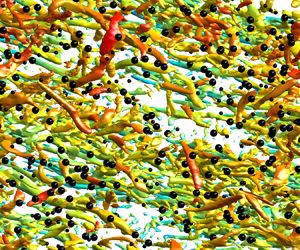
Figure 1. Visualization of case C1 at $t^+\approx 1.5\times 10^4$. The vortical structures within the lower half of the channel are visualized by the Q-criterion ($Q=25$) and coloured with instantaneous streamwise velocity normalized by the friction velocity ($u^+=u/u_\tau$). Black (white) spheres denote the larger (smaller) particles with wall distance below $h/2$ ($h=0.2$ m), where only one out of every twenty thousand particles is shown for clarity.

In comparison to the unladen case C0, we examine two cases of particle-laden turbulent channel flows: one laden with uncharged bidisperse particles (case C1) and the other with charged bidisperse particles (case C2). Notably, the choice of a bidisperse particle system is motivated by two main reasons. First, in both industrial and natural systems, particles are always polydisperse, exhibiting distinct behaviours from monodisperse particles (e.g. Zhou, Wexler & Wang 2001). Second, in many situations, such as those encountered in dust storms, the low volume fraction of particles (i.e. dilute regime) often results in only binary inter-particle collisions (Zhang & Zhou 2023; Zhang et al. 2023). Thus the mixing and dispersion of particles in the flow are typically analysed by considering the relative motion of particle pairs. Importantly, the polydisperse statistics can be derived from appropriate integrals of bidisperse statistics, weighted based on the size distribution of the particles (Dhariwal & Bragg 2018). Thus under such conditions, turbulent flows containing polydisperse particles can be effectively simplified into a bidisperse system.

In both laden cases, the particle-to-fluid density ratio for all particles is set to $\rho _p/\rho _f = 2200$, which is consistent with the density ratio of sand particles to air in natural wind-blown sand movements (Zheng 2009). The bidisperse particles consist of two distinct particle types characterized by viscous Stokes numbers $St^+=t_p/t_\nu$ with values 25 and 120, corresponding to particle diameters $164\,\mathrm {\mu }{\rm m}$ and $360\,\mathrm {\mu }{\rm m}$, respectively. Here, $t_p=d_p^2\rho _p/(18\nu \rho _f)$ and $t_\nu =\nu /u_\tau ^2$ are the particle inertial response time and fluid viscous time scale, respectively. Specifically, the dimensionless particle diameters $d_p^+=d_p/\delta _\nu$ for the larger and smaller particles are 0.45 and 0.99, respectively, both of which are smaller than the Kolmogorov scale of the fluid flow. The number of both larger and smaller particles is $1.60\times 10^7$, with corresponding bulk mean particle mass loading (volume fraction) $\overline {\phi _m}$ ($\overline {\phi _V}$) having values $2.27\times 10^{-1}$ and $0.22\times 10^{-1}$ ($1.03\times 10^{-4}$ and $0.10\times 10^{-4}$). The particle mass loading at the wall-normal location $y$ is defined as $\phi _m\equiv \rho _p/\rho _f\phi _V$ (e.g. Hwang & Eaton 2006; Yousefi et al. 2023), where $\phi _V=\sum _{i=1}^{2}{N_{p,i}V_{p,i}/(L_xL_z\,\mathrm {d}\xi )}$ is the particle volume fraction within the wall-normal location $[y-\mathrm {d}\xi /2,y+\mathrm {d}\xi /2]$, with $\mathrm {d}\xi$ being the radius of the smaller particle. Here, $N_{p,i}$ represents the total number of the $i$th particle class within this wall-normal position range, and $V_{p,i}$ denotes the volume of a particle of the $i$th particle class.

In case C2, charge transfer during inter-particle and particle–wall collisions is not considered, as in many previous studies (e.g. Di Renzo & Urzay 2018; Grosshans et al. 2021; Boutsikakis et al. 2022). Consequently, all particles carry constant surface charge density $\sigma _s=0.27\,\mathrm {\mu }{\rm C}\,{\rm m}^{-2}$, which is 0.01 times the maximum surface charge density for spherical particles in a normal atmosphere (Hamamoto, Nakajima & Sato 1992). It is well known that particle electrification exhibits a ‘size-dependent effect’, where larger particles tend to charge positively while smaller particles tend to charge negatively (Lacks & Sankaran 2011). Therefore, each larger (smaller) particle carries a charge $+0.11$ pC ($-0.02$ pC). The relative importance of particle electrical effects and particle inertia can be quantified by the electrostatic Stokes number $St_{el}$, which is defined by the ratio of the particle inertial response time $\tau _p$ to the characteristic time scale of inter-particle electrostatic interactions $t_{el}$, i.e. $St_{el}=t_p/t_{el}$. Using standard dimensional analysis, we have $t_{el}=(6 {\rm \pi}\varepsilon _0 m_p /(n q^2))^{1/2}$, where $n$ and $\varepsilon _0$ are the particle number density and the permittivity of the vacuum, respectively. In case C2, the bulk mean $St_{el}$ is $0.84\times 10^{-2}$ for the smaller particles and $5.94\times 10^{-2}$ for the larger particles, indicating a noticeable inter-particle electrostatic interaction (e.g. Grosshans et al. 2021; Boutsikakis et al. 2022; Zhang et al. 2023).

In cases C1 and C2, once the unladen case C0 reaches a fully developed state (denoted by $t^+=t/t_\nu =0$), particles are released randomly into the entire computational domain, with their initial velocities matching the fluid velocity at the particles’ positions. Subsequently, the particle-laden turbulent channel flow continues to evolve until it achieves a statistically stationary state at approximately $t^+=1.5\times 10^4$ (or equivalently, global eddy-turnover time $h/u_\tau \approx 28$). In this study, the numerical algorithm is implemented in Fortran 90 computer code and parallelized using the message passing interface based on a two-dimensional pencil-like domain decomposition (Costa 2018). The typical duration of a simulation is approximately 64 000 CPU hours on 512 cores (Intel Xeon Platinum 9242 CPU @ 2.30 GHz). In practice, ensemble averages for any statistics, denoted by angle brackets $\langle \,\cdot\, \rangle$, are performed numerically by spatial averaging within the horizontal plane, and temporal averaging over 11 equally spaced snapshots within the time interval $t^+\in [1.0\times 10^4,1.5\times 10^4]$, spanning more than nine global eddy-turnover times.

3. Results

3.1. Mean flow and fluctuating velocities

To assess whether inter-particle electrostatic forces significantly affect turbulence modulation by particles, we begin by presenting the instantaneous distribution of near-wall streamwise velocity fluctuations in the horizontal $x$–$z$ plane, as shown in figure 2. It is evident that charged and uncharged particles exhibit distinct modulation of the near-wall flow field. In all cases C0–C2, highly streamwise-elongated, alternating low- and high-speed streaks are present near the wall (e.g. Zhao et al. 2010; Zheng, Feng & Wang 2021). However, compared to the unladen case C0, when the flow is laden with uncharged particles, such streamwise-elongated flow streaks become longer and wider (Zhao et al. 2010). By contrast, when the particles are charged, the shapes of the fluid streaks are further expanded (a quantitative comparison using two-point autocorrelation functions is given in § 3.3), indicating that inter-particle electrostatic forces indeed have a dramatic influence on turbulence modulation.

Figure 2. Instantaneous snapshots of the fluctuating streamwise fluid velocity $u'^+$ in the streamwise–spanwise ($x$–$z$) planes at $t^+\approx 1.5\times 10^4$ (not to scale). (a–c) Snapshots of the fluctuating streamwise fluid velocity at $y^+=10.5$ for the cases C0, C1 and C2, respectively. (d–f) Same as (a–c) but for the fluctuating streamwise fluid velocity at $y^+=103.1$.

Figure 3(a) illustrates wall-normal profiles of the inner-scaled mean streamwise fluid velocities for various cases. Compared to case C0, the inner-scaled mean streamwise fluid velocity for case C1 exhibits a noticeable increase in the outer layer, and agrees well with numerous simulated and experimental results involving uncharged inertial particles with diameter smaller than the Kolmogorov length scales of turbulence (e.g. Pan & Banerjee 1996; Kaftori, Hetsroni & Banerjee 1998; Dritselis & Vlachos 2008; Zhao et al. 2013; Li et al. 2016; Gao et al. 2023). This increase in the inner-scaled mean velocity can be attributed to a reduction in the fluid friction velocity since the mass flow rate is kept constant for all cases. In contrast, the overall inner-scaled mean velocity for case C2 is considerably shifted towards lower values, suggesting an increase in the fluid friction velocity. For comparison, figure 3(b) displays the outer-scaled mean streamwise fluid velocities. It is shown that the outer-scaled mean velocities exhibit significant (slight, see inset) differences in the near-wall (outer) region.

Figure 3. Wall-normal profiles of the (a) inner-scaled and (b) outer-scaled mean streamwise fluid velocities for cases C0–C2. The inset shows the ratio of the mean streamwise fluid velocity between cases C1 and C0 (dashed line) and between C2 and C0 (dotted line).

It is known that the effect of particles on the mean streamwise velocity is determined by two physical mechanisms: (1) particles directly affect the local fluid velocity through interactions with turbulence; and (2) the presence of particles alters the local viscous transport, thus modifying the velocity gradient of the flow field (e.g. Kaftori et al. 1998; Peng, Ayala & Wang 2019). In such a case, particle mass loading plays a dominant role in the mean streamwise velocity. The PP-DNS studies of particle-laden turbulent channel flow conducted by Li et al. (2001) reveal that for smaller particle mass loadings ($\phi _m\sim 0.2\unicode{x2013}0.4$), particles increase the mean streamwise velocity, while the opposite effect is observed for the larger particle mass loading ($\phi _m\sim 2$).

Figure 4 shows comparisons of the wall-normal profiles of particle mass loading between cases C1 and C2. In case C1, particles tend to migrate towards the wall, resulting in the mean particle concentration (i.e. mass loading) being maximized within the viscous layer, a phenomenon known as turbophoresis (Caporaloni et al. 1975; Reeks 1983). Additionally, smaller particles exhibit stronger turbophoresis than larger ones. This can be attributed to two reasons: (1) turbophoresis is most pronounced when the particle response time scale matches the characteristic time scale of the buffer layer, corresponding to a particle Stokes number $St^+\sim 10\unicode{x2013}50$ (Sardina et al. 2012); and (2) larger particles experience inter-particle collisions due to larger volume fractions, which tend to bring the concentration profile towards a uniform profile (Johnson et al. 2020). In comparison to case C1, positively charged larger particles in case C2 exhibit an increase (decrease) in mass loading in the region $y^+\lesssim 180$ ($\kern0.7pt y^+\gtrsim 180$), while negatively charged smaller particles in case C2 show a decrease (increase) in mass loading in the region $y^+\lesssim 100$ ($\kern0.7pt y^+\gtrsim 100$). This leads to an overall increase in particle mass loading $\phi _m$ from $\lesssim 1$ to nearly 8 in the region of $y^+\lesssim 200$ (figure 4b). Such changes in particle mass loadings due to inter-particle electrostatic forces can be explained by the direction of the wall-normal electric field at the particles’ positions, $e_{y@p}$. As depicted in figure 5, the probability density functions (p.d.f.s) of $e_{y@p}$ for both smaller and larger particles are distributed at negative $e_{y@p}$ in the bulk of the channel, with a zero-mean $e_{y@p}$ only at the channel centreline. In such instances, negatively charged smaller (positively charged larger) particles experience electrostatic forces pointing towards the channel centreline (wall), resulting in an electrostatic drift towards the channel centreline (wall).

Figure 4. (a) Wall-normal profiles of particle mass loadings for the smaller and larger particles in cases C1 and C2. (b) Wall-normal profiles of the total particle mass loadings for cases C1 and C2.

Figure 5. The p.d.f.s of the wall-normal electric field at the positions of the particles $e_{y@p}$ for case C2. Here, the black solid lines and red dashed lines represent the p.d.f. contours for the smaller and larger particles, respectively.

Therefore, we can conclude that the opposite trends in modulation of mean streamwise velocity between uncharged and charged particles is attributed to substantial changes in particle mass loading induced by inter-particle electrostatic forces.

In addition to modulating the mean streamwise velocity, charged particles have a remarkable influence on turbulent fluctuations, as depicted in figure 6. In contrast to case C0, the root mean square (r.m.s.) streamwise fluctuating velocity is reduced in the near-wall region ($\kern0.7pt y^+\lesssim 20$) in the presence of uncharged particles, with a slight enhancement in the outer region ($\kern0.7pt y^+\gtrsim 20$). Conversely, the r.m.s. wall-normal and spanwise fluctuating velocities, as well as Reynolds stress, are largely diminished throughout the entire channel. These results are consistent with previous studies on turbulent channel flows laden with uncharged particles (e.g. Li et al. 2001; Dritselis & Vlachos 2008). Importantly, when compared to case C1, all r.m.s. fluctuating velocities and Reynolds stress in the region $y^+\lesssim 200$ are significantly suppressed for case C2, with negligible effects in the region $y^+\gtrsim 200$. This implies that inter-particle electrostatic forces appear to further inhibit turbulent fluctuations.

Figure 6. Wall-normal profiles of the r.m.s. (a) streamwise, (b) wall-normal and (c) spanwise fluctuating velocities, as well as (d) Reynolds stress $-\langle u'^+v'^+\rangle$ for cases C0–C2.

The attenuation of turbulence by charged particles can be explained by variations in the parameters that control turbulence modulation. For the flow and particle conditions examined herein, the main control parameters are particle Reynolds number and mass loading (Peng et al. 2019). It is widely acknowledged that: (1) particles with low Reynolds numbers suppress turbulence, whereas those with higher Reynolds numbers, typically larger than 300 for isolated particles (Hetsroni 1989; Johnson & Patel 1999) but small for particle clusters (Capecelatro et al. 2014, 2015), enhance turbulence through wake shedding (Hetsroni 1989; Yu et al. 2021); (2) as particle mass loading increases, turbulence modulation by particles becomes increasingly pronounced (Kulick et al. 1994; Li et al. 2001; Zhao et al. 2013; Costa et al. 2021). In this study, as shown in figure 7, although the particle Reynolds numbers near the wall are altered considerably when the particles are charged, their values remain below 5, indicating the absence of wake shedding. Therefore, according to the aforementioned criteria, whether particles are charged or not, they are believed to suppress turbulence fluctuations. On the other hand, the particle mass loading is significantly increased near the wall but is slightly changed in the outer region (figure 4b) when particles are charged. This results in charged particles having a substantial suppression (negligible influence) on turbulence near the wall (in the outer region) compared to the uncharged particles.

Figure 7. Wall-normal profiles of the average particle Reynolds number $\langle Re_p \rangle$ for the smaller and larger particles in cases C1 and C2.

For completeness, the basic statistics of the particulate phase are also shown in figure 8. As expected, when particles are uncharged, the smaller particles follow the fluid phase fairly well, but the larger particles travel faster than the fluid phase below $y^+\approx 15$, in line with previous studies (e.g. Li et al. 2012; Fong, Amili & Coletti 2019). When particles are charged, the mean particle streamwise velocity of the smaller particles increases, while that of the larger particles decreases below $y^+\approx 15$; both exceed the mean fluid streamwise velocity within this layer (figure 8a). As a result, the magnitude of the mean particle-to-fluid relative velocity, $\langle \Delta u^+ \rangle =\langle u_{f@p}^+ \rangle - \langle u_p^+ \rangle$, is increased (decreased) for the smaller (larger) particles (figure 8b). Under the influence of inter-particle electrostatic forces, the r.m.s. streamwise particle fluctuating velocity of the smaller particles is increased (decreased) below (above) $y^+\approx 8$, while that of larger particles is decreased (remains unchanged) below (above) $y^+\approx 30$ (figure 8c). Interestingly, the r.m.s. streamwise fluctuating velocity of the particulate phase is also larger than that of the fluid phase throughout the channel. Similar conclusions are found for the r.m.s. particle fluctuating velocity of the spanwise and wall-normal components (not shown for brevity), and particle Reynolds stress (figure 8d).

Figure 8. Wall-normal profiles of (a) the mean streamwise particle velocity $\langle u_p^+ \rangle$, (b) the mean particle-to-fluid relative velocity $\langle \Delta u^+ \rangle =\langle u_{f@p}^+ \rangle - \langle u_p^+ \rangle$, (c) the r.m.s. streamwise particle fluctuating velocity $u'_{p,rms}$ and (d) the particle Reynolds stress $-\langle u'_pv'_p \rangle$, for cases C1 and C2. Here, the dashed and dotted lines represent the corresponding statistics of the fluid phase.

3.2. Interphase momentum and energy transfer

To gain further insight, we next examine the streamwise momentum balance of the fluid phase (Picano et al. 2015; Peng et al. 2019; Costa et al. 2021; Gao et al. 2023),

(3.1)\begin{equation} \tau_T(y)=\underbrace{\rho_f \nu\,\frac{\partial \langle u \rangle}{\partial y}}_{\tau_\nu}\underbrace{\vphantom{\int_h^y \langle\,f_x\rangle \,\mathrm{d} y'}-\rho_f \langle u'v' \rangle}_{\tau_R}+\underbrace{\rho_f \int_h^y \langle\,f_x\rangle \,\mathrm{d} y}_{\tau_p}=\tau_w\left(1-\frac{y}{h}\right), \end{equation}

where $\langle\,f_x \rangle$ is the mean hydrodynamic force in the streamwise direction exerted on the fluid phase due to particles, and $\tau _T$, $\tau _\nu$, $\tau _R$ and $\tau _p$ denote the total, fluid viscous, turbulent Reynolds and particle stresses, respectively. A detailed derivation of (3.1) is provided in Appendix A.

Figure 9(a) displays the streamwise momentum balance for various cases. It is evident that the total stress $\tau _T$ behaves as a straight line with slope $-1/h$ for different cases (see inset of figure 9a), suggesting that all simulations have attained the final steady state. The fluid viscous stress $\tau _\nu$ dominates in the viscous sublayer but rapidly decreases to very small values as $y$ increases, nearly unaffected by the presence of uncharged and charged particles. For case C0, the turbulent Reynolds stress $\tau _R$ increases with increasing $y$, peaks at $y/h\approx 0.8$, and then decreases, dominating in the outer region. In the presence of particles, the turbulent Reynolds stress follows a similar trend to that of unladen flow but is substantially reduced due to momentum extraction by particles, especially when the particles are charged. The profiles of the particle stress $\tau _p$ resemble those of turbulent Reynolds stress but reach their maxima at a relatively low wall-normal location. In particular, when particles are charged, the particle stress is significantly enhanced below (and reduced above) $y/h\approx 0.3$, suggesting that inter-particle electrostatic forces facilitate the particles to extract momentum from the fluid phase near the wall.

Figure 9. (a) Wall-normal profiles of the fluid viscous (dotted lines), turbulent Reynolds (solid lines) and particle stresses (dot-dashed lines), where the black dashed line denotes $\tau _w(1-y/h)$. The inset shows the summations of the fluid viscous, turbulent Reynolds and particle stresses for various cases. Here, green, blue and red lines denote cases C0, C1 and C2, respectively. (b) Relative contributions of different stresses in the stress budget to the mean wall friction, which is normalized by that of the unladen case, namely, $1/h\int _{0}^{h}3(1-y/h)\tau _i\,{\rm d}y/(\rho _fu_{\tau,0}^2)$. Here, the contribution of the stress $\tau _i$, $i\in \{P,R,\nu \}$, is evaluated by the weighted integral $1/h\int _{0}^{h}3(1-y/h)\tau _i\,{\rm d}y$ (see Appendix B for details), and $u_{\tau,0}$ is the friction velocity for the unladen case C0.

The contribution of each stress to the overall drag is depicted in figure 9(b). For case C0, the contributions of viscous and turbulent Reynolds stresses are approximately 0.1 and 0.9, respectively. For case C1, the contribution of the viscous stress remains unchanged, but that of the turbulent Reynolds stress is reduced to approximately 0.71, resulting in the combined contribution of these two stresses (i.e. the fluid stress) being smaller than the overall drag in case C0. However, the contribution of the particle stress accounts for approximately 0.22, which counteracts the drag reduction resulting from fluid stress and leads to an overall increase in drag. For case C2, the reduction in the contribution of turbulent Reynolds stress is more prominent compared to case C1. However, due to a considerable increase in the particle stress, the overall drag is further increased. This demonstrates that inter-particle electrostatic forces increase the overall drag by indirectly enhancing the contribution of the particle stress.

Note that, compared to case C0, $u_\tau$ increases in case C2 (figure 3a), while the contribution of fluid stress to overall drag decreases (figure 9b). However, these two situations are not contradictory. Specifically, $u_\tau$ represents only the variation of $\tau _\nu$ at the wall position, and although it increases for case C2, the overall change in the wall-normal profile of $\tau _\nu$ is almost negligible. Therefore, the contribution of $\tau _\nu$ to overall drag remains constant across all cases. In contrast, for case C2, the wall-normal profile of $\tau _R$ exhibits a significant downward shift, leading to a decrease in the relative contribution of overall drag by Reynolds stress (and thus fluid stress).

It is worth remarking that although the presence of uncharged particles (case C1) enhances the total drag, it does not considerably modify the mean streamwise fluid velocity within the viscous sublayer and buffer region (figure 3a). This contrasts with many other drag modulation mechanisms. For example, when channel flow is subjected to oscillatory spanwise wall motion, the drag decreases, and the thickness of the viscous sublayer is significantly reduced (Touber & Leschziner 2012). In turbulent channel flows with a riblet surface, a maximum drag reduction is reached when the so-called ‘viscous regime’ breaks down (Garcia-Mayoral & Jiménez 2011). Similarly, in turbulent pipe flows with three-dimensional sinusoidal roughness, the increase in wall drag is manifested as a downward shift in the wall-normal profile of the mean streamwise fluid velocity (Chan et al. 2015).

Apart from momentum exchange, kinetic energy exchange between the particulate phase and the fluid phase also arises due to the presence of relative velocity between them. The amounts of kinetic energy transferred from the local fluid to a particle and from a particle to the local fluid per unit time, denoted by powers $W_p$ and $W_f$, are given by (Zhao et al. 2013; Li et al. 2016)

(3.2)\begin{gather} W_p=\frac{m_p(1+0.15\,Re_p^{0.687})}{t_p}\left(\boldsymbol{u}_{f@p}-\boldsymbol{u}_p\right)\boldsymbol{\cdot} \boldsymbol{u}_p, \end{gather}

(3.3)\begin{gather} W_f={-}\frac{m_p(1+0.15\,Re_p^{0.687})}{t_p}\left(\boldsymbol{u}_{f@p}-\boldsymbol{u}_p\right)\boldsymbol{\cdot} \boldsymbol{u}_{f@p}. \end{gather}

Therefore, the net particle dissipation $\varepsilon _p$ is expressed as the sum of $W_p$ and $W_f$:

(3.4)\begin{equation} \varepsilon_p=W_p+W_f=\frac{m_p(1+0.15\,Re_p^{0.687})}{t_p}\left(\boldsymbol{u}_{f@p}-\boldsymbol{u}_p\right)\boldsymbol{\cdot} (\boldsymbol{u}_p-\boldsymbol{u}_{f@p}). \end{equation}

Figure 10 illustrates the wall-normal profiles of powers $\langle W_p^+ \rangle$ and $\langle W_f^+ \rangle$, as well as particle dissipation $\langle \varepsilon _p^+ \rangle$. As shown in figures 10(a–c), in the case of C1, values of $\langle W_p^+ \rangle$, $\langle W_f^+ \rangle$ and $\langle \varepsilon _p^+ \rangle$ for larger particles (i.e. $St^+=120$) are much larger than those for small particles (i.e. $St^+=25$), especially in the near-wall region, in agreement with the results of Gao et al. (2023). This discrepancy arises because larger particles exhibit a greater particle-to-fluid relative velocity in the near-wall region (Kulick et al. 1994; Vance, Squires & Simonin 2006; Fong et al. 2019). Interestingly, in the case of C2, values of $\langle W_p^+ \rangle$, $\langle W_f^+ \rangle$ and $\langle \varepsilon _p^+ \rangle$ for smaller particles are significantly enhanced, while those for larger particles are notably suppressed. This occurs because inter-particle electrostatic forces tend to enhance (inhibit) the particle-to-fluid relative velocity of smaller (larger) particles in the near-wall region (see figure 8b). However, compared to case C1, the total $\langle W_p^+ \rangle$ and $\langle W_f^+ \rangle$ are considerably enhanced when particles are charged (figures 10d,e). It should be emphasized that in the presence of particles, the total particle dissipation $\langle \varepsilon _p^+ \rangle$ is non-zero, indicating that particles induce additional energy dissipation. Furthermore, when particles are charged, the extra dissipation caused by the particles is remarkably strengthened below $y^+\approx 110$ (see figure 10f).

Figure 10. (a–c) Wall-normal profiles of the normalized powers $\langle W_p^+ \rangle$ and $\langle W_f^+ \rangle$, as well as particle dissipation $\langle \varepsilon _p^+ \rangle$ for the smaller and larger particles, in cases C1 and C2. (d–f) Same as (a–c), but for the total power and particle dissipation. Here, all powers and particle dissipations are normalized by $m_p u_\tau ^2/t_p$.

Similar to the transfer of kinetic energy, the fluctuating feedback force exists in the governing equation of the turbulent kinetic energy budget, and generally exhibits a dissipative effect. The balance equation of the turbulent kinetic energy $K=\langle \boldsymbol {u}' \boldsymbol {\cdot } \boldsymbol {u}' \rangle /2$ for the channel flow is given by

(3.5)\begin{equation} P_K-D_K-\epsilon_K+\varPsi_K=0, \end{equation}

where

(3.6)\begin{gather} P_K={-}\langle u^{\prime} v^{\prime} \rangle\,\frac{\partial \langle u \rangle }{\partial y}, \end{gather}

(3.7)\begin{gather} D_K=\frac{\partial}{\partial y}\left(\frac{1}{2}\,\langle (\boldsymbol{u}' \boldsymbol{\cdot} \boldsymbol{u}') v' \rangle+\frac{\langle p' v'\rangle}{\rho_f}-\nu\,\frac{\partial \langle K \rangle}{\partial y}\right), \end{gather}

(3.8)\begin{gather} \epsilon_K=\nu \langle \boldsymbol{\nabla} \boldsymbol{u}' \boldsymbol{:} \boldsymbol{\nabla} \boldsymbol{u}' \rangle, \end{gather}

(3.9)\begin{gather} \varPsi_K=\langle \boldsymbol{u}' \boldsymbol{\cdot} \boldsymbol{f}' \rangle. \end{gather}

Here, $P_K$, $D_K$, $\epsilon _K$ and $\varPsi _K$ represent the turbulent production, total turbulent diffusion, turbulent viscous dissipation and particle-induced energy sink term, respectively. The production term $P_K$ represents the generation of velocity fluctuations through mean shear, which is a source term in (3.5). The diffusion term $D_K$ redistributes energy with no net contribution. The energy injected via $P_K$ is dissipated by turbulent dissipation $\epsilon _K$ and particle-induced energy sink $\varPsi _K$.

The turbulent kinetic energy budget is depicted in figure 11. It is apparent that all terms in (3.5) are considerably influenced by the presence of particles. The addition of uncharged particles results in a reduction in the magnitudes of turbulent production, diffusion and dissipation. When particles are charged, these reductions become more prominent. The substantial reduction in turbulent production necessitates a reduction in viscous dissipation. In particular, the particle-induced energy sink plays a crucial role in turbulence attenuation. In a thin layer adjacent to the wall, where turbulent fluctuations are weak, fluid velocity fluctuations are produced mainly by particles. Therefore, velocity fluctuations of the fluid and particles are expected to be positively correlated within this thin layer, resulting in a positive $\varPsi _K$ (see Vreman 2015). However, $\varPsi _K$ is negative in the bulk of the channel flow, acting as a sink for turbulent kinetic energy (figure 11d). In short, inter-particle electrostatic forces suppress turbulent production and enhance the particle-induced energy sink, thereby attenuating turbulence.

Figure 11. Turbulence kinetic energy budget in the near-wall region: (a) turbulence production $P_K^+$, (b) total diffusion $D_K^+$, (c) turbulence dissipation $\varepsilon ^+$, and (d) particle-induced energy source term $\varPsi _K^+$. Here, all terms are normalized by $u_\tau ^4/\nu$.

3.3. Premultiplied spectra and autocorrelation functions

To elucidate the role of inter-particle electrostatic forces in the modulating turbulence structure, we end by quantifying the premultiplied spectra and two-point autocorrelation functions of the fluctuating streamwise fluid velocity in this subsection. Figure 12 shows the premultiplied one-dimensional $u$-spectra $k_x\varPhi _{uu}/u_\tau ^2$ and $k_z\varPhi _{uu}/u_\tau ^2$, where $\varPhi _{uu}=\langle \hat {u}'(k_z)\, \hat {u}'^\ast (k_z)\rangle$, with $\widehat {(\ )}$ and $(\ )^\ast$ representing the Fourier modes and complex conjugate, respectively (Pope 2000). For case C0 (figures 12a,d), the premultiplied spectra $k_x\varPhi _{uu}/u_\tau ^2$ and $k_z\varPhi _{uu}/u_\tau ^2$ exhibit a noticeable inner peak at wall-normal location $y^+\approx 13$ and wavelengths $\lambda _x^+\approx 1000$ and $\lambda _z^+\approx 100$, consistent with existing results (Del Alamo & Jiménez 2003; Wang & Richter 2019b). The emergence of this inner peak is created by the self-sustaining near-wall cycle (e.g. Jiménez & Pinelli 1999; Schoppa & Hussain 2002; Hutchins & Marusic 2007). In addition, this inner peak corresponds to a spatial length of approximately $1.85h$ in the streamwise direction, and is commonly referred to as large-scale motions (LSMs; see Guala, Hommema & Adrian 2006). Notably, we do not observe distinct outer peaks in the premultiplied spectra, which correspond to the streamwise length scales exceeding $O(3h)$, and are generally termed very-large-scale motions or superstructures (Guala et al. 2006; Hutchins & Marusic 2007; Wang & Zheng 2016). This happens because the energy content in the outer region continuously increases with increasing Reynolds number $Re_\tau$, therefore outer peaks are typically more prominent at $Re_\tau \geqslant 1800$ (Duan et al. 2020; Yao, Chen & Hussain 2022). For case C1, although the wall-normal location of the inner peak remains almost unchanged, the peaks are shifted towards larger streamwise and spanwise wavelengths (i.e. $\lambda _x^+\approx 1382$ and $\lambda _z^+\approx 133$), and their magnitudes are significantly reduced (figures 12b,e).

Figure 12. Premultiplied $u$-spectra as a function of wavelength and wall-normal location $y^+$: (a) $k_x\varPhi _{uu}/u_\tau ^2$ for case C0, (b) $k_x\varPhi _{uu}/u_\tau ^2$ for case C1, (c) $k_x\varPhi _{uu}/u_\tau ^2$ for case C2, (d) $k_z\varPhi _{uu}/u_\tau ^2$ for case C0, (e) $k_z\varPhi _{uu}/u_\tau ^2$ for case C1, and (f) $k_z\varPhi _{uu}/u_\tau ^2$ for case C2. Here, $\lambda _x^+$ and $\lambda _z^+$ denote streamwise and spanwise wavelengths, respectively. The values are normalized by the maximum value of the unladen flow. The plus signs (i.e. $+$) mark the peaks of the spectra.

It is demonstrated that inertial particles disrupt the self-sustaining near-wall cycle, where the dominant structures are the streamwise velocity streaks and quasi-streamwise vortices. Therefore, the changes in the premultiplied $u$-spectra $k_x\varPhi _{uu}/u_\tau ^2$ and $k_z\varPhi _{uu}/u_\tau ^2$ by uncharged particles can be physically explained as follows: uncharged high-inertia particles of $St^+\gtrsim O(30\unicode{x2013}50)$ (i.e. smaller and larger particles in this study; see table 2) tend to reduce the strength and number of the quasi-streamwise vortices, as well as streamwise vorticity stretching and lift-up effects (Wang & Richter 2019a); as a result, the streamwise velocity streaks are thickened, but their fluctuating amplitudes are suppressed (Zhao et al. 2010), which is reflected by a weaker premultiplied spectrum peaked at a larger wavelength.

Additionally, since the particle mass loading close to the wall is increased by the inter-particle electrostatic forces (figure 4b), the thickening of the streamwise velocity streaks and the suppression of the strength of the quasi-streamwise vortices are even more pronounced for case C2. Therefore, the weakest spectral peaks among cases C0–C2 are located at $\lambda _x^+\approx 2764$ and $\lambda _z^+\approx 185$ (figures 12c,f). In short, inter-particle electrostatic forces seem to increase the length scale of LSMs in both the streamwise and spanwise directions, but reduce the intensity of LSMs in terms of indirect modulations of the self-sustaining near-wall cycle.

To uncover the underlying physical mechanisms, we turn to evaluating the spectral production and feedback terms for the streamwise turbulent kinetic energy (TKE) and Reynolds stress budgets. Figure 13 displays the spectral production terms $\hat {P}_{11}=-\operatorname {Re}(\langle \hat {u}'(k_z, y)\,\hat {v}'^\ast (k_z, y)\rangle ) \,\mathrm {d} \langle u \rangle / \mathrm {d}y$ for the streamwise TKE $\langle u'u' \rangle$ budget, and $\hat {P}_{12}=-\langle \hat {v}'(k_z, y)\,\hat {v}'^\ast (k_z, y)\rangle \,\mathrm {d} \langle u \rangle / \mathrm {d} y$ for the Reynolds stress $\langle u'v' \rangle$ budget, as a function of spanwise wavelength $\lambda _z^+$ and wall-normal location $y^+$. Here, $\operatorname {Re}(\cdot )$ represents the real part of a complex number. For all cases C0–C2, $\hat {P}_{11}$ is positive, whereas $\hat {P}_{12}$ is negative (because of $\langle u'v' \rangle <0$) throughout the entire channel. The overall shapes of $\hat {P}_{11}$ resemble those of the premultiplied spectra $k_z\varPhi _{uu}/u_\tau ^2$. However, the patterns of $\hat {P}_{12}$ differ significantly from those of $\hat {P}_{11}$. For case C1, the magnitudes of both $\hat {P}_{11}$ and $\hat {P}_{12}$ are weakened, especially at the inner peaks (figures 13b,e). Again, this effect is more pronounced for case C2 (figures 13c,f), implying that inter-particle electrostatic forces suppress the production of $\langle u'u' \rangle$ and $\langle u'v' \rangle$ around the scales of LSMs. It is important to note that the same conclusions can be drawn for $\hat {P}_{11}$ and $\hat {P}_{12}$ as functions of the streamwise wavelength and wall-normal location, but they are not presented here and below for the sake of clarity.

Figure 13. Spectral production contribution to the streamwise TKE budget $\hat {P}_{11}$ and Reynolds stress budget $\hat {P}_{12}$: (a) $\hat {P}_{11}$ for case C0, (b) $\hat {P}_{11}$ for case C1, (c) $\hat {P}_{11}$ for case C2, (d) $\hat {P}_{12}$ for case C0, (e) $\hat {P}_{12}$ for case C1, and ( f) $\hat {P}_{12}$ for case C2. Here, $\hat {P}_{11}$ and $\hat {P}_{12}$ are normalized by $u_\tau ^3/\delta _\nu$. The plus signs (i.e. $+$) mark the peaks of the spectra.

Figure 14 shows the spectral feedback terms $\hat {\varPsi }_{11}=\operatorname {Re}(\langle \widehat {F'_x}(k_z, y)\,\hat {u}'^\ast (k_z, y)\rangle )$ for the the streamwise TKE $\langle u'u' \rangle$ budget, and $\hat {\varPsi }_{12}=\operatorname {Re}(\langle \widehat {F'_x}(k_z, y)\,\hat {v}'^\ast (k_z, y)\rangle + \langle \widehat {F'_y}(k_z, y)\,\hat {u}'^\ast (k_z, y)\rangle )$ for the Reynolds stress $\langle u'v' \rangle$ budget, where $F'_x$ and $F'_y$ denote the fluctuating particle feedback forces on the fluid phase in the streamwise and wall-normal directions, respectively. Interestingly, the spectral feedback terms $\hat {\varPsi }_{11}$ and $\hat {\varPsi }_{12}$ behave quite differently compared to the production terms. It is clear that for cases C1 and C2, $\hat {\varPsi }_{11}$ is negative in the bulk of the channel, but positive within the viscous sublayer (i.e. $y^+\lesssim 5$) at large spanwise wavelengths (figures 14a,b). The negative part of $\hat {\varPsi }_{11}$ is peaked at $y^+\approx 15$ and $\lambda _z^+\approx 230$, while the positive part of $\hat {\varPsi }_{11}$ is peaked at $y^+\approx 1.5$ and $\lambda _z^+\approx 750$. This bipolar behaviour is a result of the interplay between smaller ($St^+=25$) and larger ($St^+=120$) particles embedded in the fluid phase in cases C1 and C2 (see table 2). This is because Wang & Richter (2019b) have demonstrated that $\hat {\varPsi }_{11}$ appears positive for the small-inertial particles ($St^+=2.4\unicode{x2013}24.2$), but negative for large-inertial particles ($St^+=60.5\unicode{x2013}908$). In contrast, $\hat {\varPsi }_{12}$ is positive throughout the entire channel and is peaked at the same wavelength but at a relatively high wall-normal location, suggesting a different role for $\hat {\varPsi }_{12}$ compared to $\hat {\varPsi }_{11}$ (figures 14c,d). By comparing cases C1 and C2, we find that the negative part of $\hat {\varPsi }_{11}$ and the whole of $\hat {\varPsi }_{12}$ are both substantially enhanced when particles are charged, even though the positive part of $\hat {\varPsi }_{11}$ shifts toward the wall and widens in the wavelength domain. This suggests that inter-particle electrostatic forces enhance the particle feedback around the scales of the LSMs, in accord with the enhancements of particle dissipation (see figure 10). Combining the results from figures 13 and 14, we can conclude that the attenuation of the intensity of LSMs by charged particles is caused by both reduction of turbulent production and enhancement of particle dissipation around the scales of LSMs by inter-particle electrostatic forces.

Figure 14. Spectral feedback term contribution to: (a) the streamwise TKE budget $\hat {\varPsi }_{11}$ for case C1, (b) the streamwise TKE budget $\hat {\varPsi }_{11}$ for case C2, (c) the Reynolds stress budget $\hat {\varPsi }_{12}$ for case C1, and (d) the Reynolds stress budget $\hat {\varPsi }_{12}$ for case C2. Here, $\hat {\varPsi }_{11}$ and $\hat {\varPsi }_{12}$ are normalized by $u_\tau ^3/\delta _\nu$. The plus signs (i.e. $+$) mark the peaks of the spectra.

In contrast to premultiplied $u$-spectra, the two-point autocorrelation function of the fluctuating streamwise fluid velocity measures the average spatial fluid structure (Ganapathisubramani et al. 2005; Hutchins & Marusic 2007). Such autocorrelation functions in the streamwise–spanwise ($x$–$z$) and streamwise–wall-normal ($x$–$y$) planes, $R_{uu}^{x-z}$ and $R_{uu}^{x-y}$, are respectively defined by

(3.10)\begin{gather} R_{uu}^{x-z}(\Delta x, \Delta z, y_{ref})=\frac{\langle u'(x, z, y_{ref})\,u'(x+\Delta x, z+\Delta z, y_{ref})\rangle}{\langle {u'}^2(x, z, y_{ref})\rangle}, \end{gather}

(3.11)\begin{gather} R_{uu}^{x-y}(\Delta x, y, y_{ref})=\frac{\langle u'(x, y_{ref},z)\,u'(x+\Delta x, y,z)\rangle}{\langle {u'}^2(x, y_{ref},z)\rangle^{1/2}\langle {u'}^2(x+\Delta x, y,z)\rangle^{1/2}}, \end{gather}

where $y_{ref}$ is the reference wall-normal location at which the autocorrelation function is evaluated, and $\Delta x$ and $\Delta z$ are the in-plane streamwise and spanwise separations, respectively.

Figures 15 and 16 display comparisons of the autocorrelation functions between cases C0 and C1, and between C1 and C2, respectively. It can be seen that for all cases C0–C2, the autocorrelation function $R_{uu}^{x-z}$ is highly elongated in the streamwise direction within the near-wall region (figures 15a and 16a), in line with the streaky structures observed in the instantaneous fluid velocity (figures 2a–c). However, these anisotropic streaky structures become longer and wider in the presence of uncharged particles (figure 15a), and this effect is more pronounced when the particles are charged (figure 16a), consistent with figures 2(a–c). This structural expansion can also be observed in the outer layer, but with relatively slight variations (figures 15b and 16b), which are caused by the disruptions of the self-sustaining near-wall cycle by larger particles, as discussed earlier.

Figure 15. Two-point autocorrelation functions of the fluctuating streamwise fluid velocity: (a) in the $x$–$z$ plane, $R_{uu}^{x-z}$ with $y_{ref}/h=1.95\times 10^{-2}$ (equivalent to $y_{ref}/\delta _\nu =10.5$); (b) in the $x$–$z$ plane, $R_{uu}^{x-z}$ with $y_{ref}/h=0.19$ (equivalent to $y_{ref}/\delta _\nu =103.1$); (c) in the $x$–$y$ plane, $R_{uu}^{x-y}$ with $y_{ref}/h=1.95\times 10^{-2}$; and (d) in the $x$–$y$ plane, $R_{uu}^{x-y}$ with $y_{ref}/h=0.19$. Here, dotted and solid lines denote cases C0 and C1, respectively.

Figure 16. Same as figure 15, but for the comparisons of autocorrelation functions between cases C1 and C2, which are denoted by the solid and dashed lines, respectively.

Aside from $R_{uu}^{x-z}$, $R_{uu}^{x-y}$ is also influenced by the presence of uncharged and charged particles. As shown in figures 15(c,d) and 16(c,d), the inclined structures of the fluid velocity in the wall-normal planes become flatter due to the presence of particles, particularly in the case of flow laden with charged particles. The physical mechanisms responsible for this structural flattening are not yet fully understood. A possible explanation is that in the streamwise–wall-normal planes, particles form inclined rod-like clusters residing above the fluid structures (Zhu et al. 2021), which are expected to lower the downstream edge of the fluid structures towards the wall (Salesky & Anderson 2020). In summary, it appears that inter-particle electrostatic forces lead to the expansion of average streaky fluid structures in the streamwise–spanwise planes, and the flattening of average inclined fluid structures in the streamwise–wall-normal planes.

4. Conclusions

In this paper, utilizing point-particle direct numerical simulations, we investigate how charged bidisperse particles affect the turbulent intensity and structure of horizontal channel flows at friction Reynolds number $Re_\tau \approx 540$. A total of $3.2\times 10^7$ bidisperse particles are released into the fluid flow, which is made up of two kinds of species, with equal amounts and mass density, but different diameters. The particle-to-fluid density ratio is set to match that of natural sand particles, i.e. $\rho _p/\rho _f = 2200$ (Zheng 2009). The diameter of the larger particles is $360\,\mathrm {\mu }{\rm m}$ (0.99 in viscous units), and that of the smaller ones is $164\,\mathrm {\mu }{\rm m}$ (0.45 in viscous units), corresponding to viscous Stokes numbers $St^+=25$ and 120, respectively. We consider three cases: an unladen flow (C0), a flow laden with uncharged particles (C1), and a flow laden with charged particles (C2). In case C2, the larger particles are positively charged, while the smaller ones are negatively charged, in accordance with the ‘size-dependent’ phenomena in particle electrification (Lacks & Sankaran 2011; Zheng 2013). The main findings of the present study are summarized below.

Compared to case C0, the wall-normal profile of the inner-scaled mean streamwise fluid velocity is noticeably increased in the outer layer for case C1 due to a decrease in the fluid friction velocity. In contrast, the overall profile of the mean streamwise velocity is substantially shifted towards lower values. This opposite trend in the modulation of the inner-scaled mean streamwise fluid velocity for cases C1 and C2 can be explained by the substantial enhancement of particle mass loading below $y^+ \approx 180$ when particles are charged. It has been reported previously that particles with small and large mass loadings result in opposite effects on turbulence modulation (Li et al. 2001). As expected, turbulent intensity is inhibited by the presence of uncharged particles. However, in comparison to case C1, the root mean square streamwise, spanwise and wall-normal fluctuating velocities, as well as Reynolds stress for case C2, are remarkably diminished below $y^+ \approx 200$, with slight changes above $y^+ \approx 200$. This suggests that inter-particle electrostatic forces seem to further suppress turbulent intensities. The main reasons are twofold: the particle Reynolds numbers of the considered sub-Kolmogorov-sized particles are smaller than 5 and thus consistently suppress turbulent intensity, regardless of the presence of uncharged or charged particles; inter-particle electrostatic forces alter particle mass loading considerably in the near-wall region but negligibly in the outer region.

Even though viscous stress is found to be unaffected by the presence of uncharged and charged particles, turbulent Reynolds stress is significantly decreased, especially for case C2. Meanwhile, particle stress for case C1 is largely enhanced in case C2. This phenomenon indicates that inter-particle electrostatic forces promote the particles to extract momentum from the fluid phase. In particular, compared to case C1, although the contribution of turbulent Reynolds stress to the overall drag for case C2 is significantly reduced, due to a substantial increase in particle stress, the total overall drag for case C2 is further increased. Consequently, inter-particle electrostatic forces enhance the overall drag through an indirect mechanism: strengthening the contribution of the particle stress. Besides momentum exchange, inter-particle electrostatic forces also appear to facilitate kinetic energy transfer between particles and the fluid phase, leading to a considerable enhancement of extra dissipation by particles. Accordingly, the further reduction of turbulence intensity by charged particles results from enhanced momentum extraction and extra particle dissipation caused by inter-particle electrostatic forces.

The structural characteristics of the fluid phase are finally quantified by analysing premultiplied spectra and autocorrelation functions. It is shown that the large-scale motions (LSMs), corresponding to the inner peaks of the premultiplied spectra of streamwise fluid velocity, are shifted towards larger streamwise and spanwise scales, but their intensity is weakened in the presence of uncharged particles. These increases in length scale and decreases in intensity of LSMs are more pronounced when particles are charged. Based on the analysis of the spectral production and feedback terms for the streamwise turbulent kinetic energy and Reynolds stress budgets, we find that the attenuation of intensity of LSMs is due to the decrease in turbulent production and the increase in particle feedback around the scales of the LSMs by inter-particle electrostatic forces. Furthermore, the average spatial fluid structures are quantified using two-point autocorrelation functions. It is found that inter-particle electrostatic forces appear to expand the streaky fluid structures in the wall-parallel planes and flatten the inclined fluid structures in the wall-normal planes.

One limitation of this study is its focus solely on exploring the difference in turbulence modulation between uncharged particles and charged particles with a specific charge level, at a given particle volume fraction. Future work warrants further investigation into exploring the quantitative laws and underlying physical mechanisms of particle-induced turbulence modulation, and even relaminarization, under different particle volume fractions and charges.