Effects of wall temperature on hypersonic shock wave/turbulent boundary layer interactions

Abstract

Wall temperature has a significant effect on shock wave/turbulent boundary layer interactions (STBLIs) and has become a non-negligible factor in the design process of hypersonic vehicles. In this paper, direct numerical simulations are conducted to investigate the wall temperature effects on STBLIs over a 34° compression ramp at Mach number 6. Three values of the wall-to-recovery-temperature ratio (0.50, 0.75 and 1.0) are considered in the simulations. The results show that the size of the separation bubble declines significantly as the wall temperature decreases. This is because the momentum profile of the boundary layer becomes fuller with wall cooling, which means the near-wall fluid has a greater momentum to suppress flow separation. An equation based on the free-interaction theory is proposed to predict the distributions of the wall pressure upstream of the corner at different wall temperatures. The prediction results are generally consistent with the simulation results (Reynolds number Re_τ ranges from 160 to 675). In addition, the low-frequency unsteadiness is studied through the weighted power spectral density of the wall pressure and the correlation between the upstream and downstream. The results indicate that the low-frequency motion of the separation shock is mainly driven by the downstream mechanism and that wall cooling can significantly suppress the low-frequency unsteadiness, including the strength and streamwise range of the low-frequency motions.

1. Introduction

Shock wave/turbulent boundary layer interactions (STBLIs) are complex flow phenomena that have been widely studied in recent decades (Dolling 2001). STBLIs commonly occur in the internal or external flow of supersonic or hypersonic vehicles and have an important influence on aerodynamic characteristics. In STBLIs, the shock wave can induce the flow separation of the turbulent boundary layer, and then the flow becomes unsteady and difficult to predict. The unsteadiness is manifested as motions with various frequencies and scales. It is particularly noteworthy that the characteristic frequency of the separation shock motion is much lower than that of the upstream turbulent boundary layer (Clemens & Narayanaswamy 2014) and that this large-scale and low-frequency motion can adversely affect supersonic flight.

The problem of hypersonic STBLIs is one of the most noteworthy focuses in high-speed flight. For example, hypersonic STBLIs exist inside scramjet engines and possibly cause flow separation. The separation can lead to the engine inlet blockage and make the engine unable to function. In addition, hypersonic STBLIs can generate local high heat flux, which may result in the failure of thermal protection on the surface of a hypersonic vehicle. Therefore, before studying and designing a hypersonic vehicle, it is important to understand the mechanisms of hypersonic STBLIs and make relatively accurate estimates of their potential impact.

Most previous studies on STBLIs, including experimental (Dolling & Murphy 1983; Erengil & Dolling 1991; Humble, Scarano & Van Oudheusden 2009) and numerical investigations (Pirozzoli & Grasso 2006; Wu & Martin 2007, 2008; Li et al. 2010), have been carried out under the condition of an adiabatic wall (the wall-to-recovery-temperature ratio ${T_w}/{T_r} = 1$). In recent years, the wall temperature has become a research emphasis because of its significant effects on compressible boundary layers and STBLIs. In the design process of hypersonic aircraft, there are some differences between the temperature of wind tunnel tests and that of actual flights, so the mechanism and law of the wall temperature effects on aerodynamic characteristics are the concern of designers.

Early research on wall temperature effects was mainly based on experiments. Spaid & Frishett (1972) conducted an experimental study of STBLIs in a compression corner at Mach 2.9 with ${T_w}/{T_r}$ ranging from 0.47 to 1.05. These scholars found that the static pressure distribution was not sensitive to the presence of small regions of separated flow and that a colder wall could reduce the separation distance. Jaunet, Debieve & Dupont (2014) analysed the wall temperature effects on the incident shock turbulent interactions at Mach 2.3 through experiments. Their results showed that wall heating had a great effect on the low-frequency motion and size of the interaction, but a small effect on the separation onset. Recently, numerical studies of the wall temperature effects have been gradually increasing. For example, Bernardini et al. (2016) studied the effects of the wall temperature on incident shock interactions through direct numerical simulations (DNSs), considering cold, adiabatic and hot walls. Their research showed that wall cooling influenced the upstream flow and separation bubble, leading to a decrease in the characteristic scales of the interaction. In addition, heat transfer was significantly amplified in the interaction region, and the thermal and dynamic loads increased as the wall cooled. Zhu et al. (2017) conducted numerical simulations of STBLIs in a 24° compression corner at Mach 2.9 with four different wall temperatures. These researchers found that the scale of the separation flow increased significantly with increasing wall temperature, consistent with the phenomena of previous studies. In addition, they derived a semi-theoretical formula to quantitatively describe the size of the separation bubble under different wall thermal conditions.

In general, these studies have achieved success with regards to the wall temperature effects on STBLIs. In addition, Duan, Beekman & Martin (2010) and Xu et al. (2021) studied the wall temperature effects on hypersonic turbulent boundary layers through DNSs. Nevertheless, there are relatively few studies regarding the wall temperature effects on STBLIs under hypersonic conditions, especially through DNS. In hypersonic flow, the compressibility of turbulence is much stronger than that in supersonic conditions. According to Morkovin's hypothesis (1962), under adiabatic wall conditions, the essential dynamics of supersonic compressible boundary layers at moderate Mach numbers (M < 5) is similar to that in incompressible flow. Although the applicability of this hypothesis was confirmed in some previous studies (Maeder, Adams & Kleiser 2001; Pirozzoli, Grasso & Gatski 2004), it is not necessarily valid under non-adiabatic hypersonic conditions. In addition, hypersonic STBLIs are often accompanied by strong shock waves and severe aerodynamic and aerothermal loads, which is quite different from the case at a low Mach number. Therefore, it is difficult for many turbulence models to simulate hypersonic STBLIs accurately (Roy & Blottner, 2006). Establishing a turbulence database through DNS to support turbulence models in hypersonic STBLIs is highly valuable.

Compared with the DNSs of hypersonic turbulent boundary layers or STBLIs at supersonic regime, the DNSs of hypersonic STBLIs are much more difficult because the latter usually require larger grid sizes and more robust numerical schemes. On the one side, compared with hypersonic turbulent boundary layers, the flow fields of hypersonic STBLIs are much more complex, including separation bubbles, shock waves, cross-flows, Görtler-like vortices and so on. To exactly simulate these structures, a larger computational domain and higher resolution of grids are usually necessary, which lead to a greater grid size. On the other side, the shock waves in hypersonic STBLIs are usually much stronger than those in supersonic STBLIs, so the simulations cannot be sustainable if the shock-capturing schemes are not robust enough. In general, the study of wall temperature effects on hypersonic STBLIs is meaningful and challenging.

In this study, we conduct DNSs of STBLIs in a 34° compression ramp at Mach 6 with three different wall temperatures ranging from ${T_w}/{T_r} = 0.50$ to ${T_w}/{T_r} = 1.0$. In § 2, the numerical methods are introduced, including the numerical schemes, computational parameters and grid settings. In § 3, we verify the reliability of the results, analyse the flow structure and low-frequency unsteadiness, and derive equations to predict the wall pressure distribution when the wall temperature changes. The conclusions are given in § 4.

2. Methodology

2.1. Numerical methods

The high-precision finite difference solver OpenCFD-SCU (Open Computational Fluid Dynamic code for Scientific Computation with GPU system) developed by Dang et al. (2022a,b) is adopted for the present study. OpenCFD-SCU is a heterogeneous parallel program developed based on the solver OpenCFD-SC (Open Computational Fluid Dynamic code for Scientific Computation). These two solvers have been applied in the DNS of wall turbulence and STBLIs in previous studies and their reliability has been verified (see table 1). OpenCFD-SCU is used to solve the compressible three-dimensional Navier‒Stokes equations in a curvilinear coordinate system, where Jacobian terms are included. The specific form of the equations can be found in the research of Dang et al. (2022a). All variables are non-dimensionalised with the reference length (set to 1 mm), and the density ρ_∞, velocity U_∞ and temperature T_∞ of the free stream.

Table 1. Previous studies using OpenCFD-SC or OpenCFD-SCU.

The hybrid difference scheme (Dang et al. 2022a) and eighth-order central difference scheme are used to calculate the convection and viscous fluxes, respectively. It is worth mentioning that the characteristic-based Steger–Warming splitting (Steger & Warming 1981) is used for the convection terms. The hybrid difference scheme is composed of the seventh-order upwind linear scheme (UDL7), the seventh-order weighted essentially non-oscillatory scheme (WENO7) and the fifth-order weighted essentially non-oscillatory scheme (WENO5) (Jiang & Shu 1996). Among them, UDL7 has the lowest numerical dissipation, followed by WENO7, and WENO5 has the highest numerical dissipation. In the present simulation of hypersonic STBLIs, UDL7 and WENO7 lack robustness in the reattachment region and are unable to make the simulation stable and sustainable; WENO5 has enough robustness to maintain a sustainable simulation, but its numerical dissipation is significantly higher than WENO7. Therefore, in the present cases, the classical WENO cannot balance the low numerical dissipation and high robustness. To solve this problem, we developed the hybrid scheme, combining the advantages of UDL7, WENO7 and WENO5. The modified shock sensor based on the research of Jameson, Schmidt & Turkel (1981) is applied to judge whether the local flow field is smooth. Specifically, the value of the shock sensor is calculated based on the pressure gradient, and two thresholds are set accordingly. When the value of the shock sensor is in a certain range (determined by the two thresholds), the hybrid scheme will select a corresponding scheme among UDL7, WENO7 and WENO5. More details on the scheme selection can be found in the research of Dang et al. (2022a). By doing this, UDL7, WENO7 and WENO5 are adopted for the smooth, unsmooth and extremely unsmooth regions, respectively, to ensure both accuracy and robustness. WENO5 is also adopted for the flux calculation near the boundaries. When a subtemplate of WENO5 uses a point outside the boundary, the weight of this subtemplate is forced to 0, which means a lower-order scheme is used near the boundaries (Dang et al. 2022a). In addition, the third-order total-variation-diminishing Runge‒Kutta method is applied for the time integration.

2.2. Flow parameters and mesh set-up

The computational models are hypersonic turbulent boundary layers over a 34° compression ramp with three different wall thermal conditions (see figure 1). The free-stream parameters of these three cases are the same, including Mach number M_∞ = 6, unit Reynolds number Re_∞ = 20 000/mm and static temperature T_∞ = 79 K. These three cases are given in table 2, where the recovery temperature is defined as ${T_r} = {T_\infty }(1 + r(\gamma - 1)M_\infty ^{\; 2}/2)\; = \; 585\;\textrm{K}$ (the temperature recovery coefficient r = 0.89). The fluid is regarded as the calorically perfect gas in the simulations. The specific heat ratio γ and Prandtl number Pr are set as constants during the computation, i.e. γ = 1.4 and Pr = 0.70. Because of the total temperature ${T_{0\infty }} = {T_\infty }(1 + (\gamma - 1)M_\infty ^{\; 2}/2) = 647.8\;\textrm{K}$, the local instantaneous temperature might exceed 600 K. Technically, above 600 K, γ gradually deviates from the constant of 1.4, considering the high-temperature real gas effects (Anderson 1982). The present research ignores this departure from the calorically perfect gas assumption.

Figure 1. Diagram of the computational domain and mesh: ${L_y}$ and ${L_z}$ represent the height and width of the computational domain, respectively; ${L_{x1}}$ and ${L_{x2}}$ represent the lengths of the flat-plate in the flat-plate region and corner region, respectively; ${L_{x3}}$ represents the length of the ramp in the corner region.

Table 2. Mesh number and resolution.

The wall temperature significantly affects the friction Reynolds number ($R{e_\tau }$) of the turbulent boundary layer (Duan et al. 2010). Therefore, to ensure that each case has similar grid resolutions ($\Delta {x^ + },\;\Delta {y^ + }$ and $\Delta {z^ + }$) in terms of wall units and sufficient computational domains, the computational domains and grid settings are different for various wall temperatures, as shown in table 2. In addition, each case has two sets of grids with different resolutions to verify the mesh independence. The resolution of the fine mesh is approximately one-third higher than that of the corresponding coarse mesh in the x, y and z directions. In each case, $L_z^ + $, the spanwise computational domain normalised by the wall units of the undisturbed boundary layer, exceeds 1000. The computational domain is divided into the flat-plate region, corner region and buffer region, as shown in figure 1. The grids are locally refined along the streamwise direction in the corner region and stretched exponentially in the buffer region, as shown in figure 2.

Figure 2. Diagram of Mesh 3-1 (x–y plane). The mesh is plotted every 20 points in both x and y directions.

We use the isothermal no-slip boundary with the corresponding wall temperature on the wall. A blowing and suction disturbance is added to stimulate the boundary layer transition. The formula and parameters of the disturbance are based on the research of Pirozzoli et al. (2004), but some parameters are reset, including the amplitude A = 0.2 and the number of spanwise waves l_max = 1. All these parameters remain consistent under different wall temperature conditions. In the cases of ${T_w}/{T_r} = 0.75$ and 1.0, the blowing-suction area ranges from x = −380 mm to x = −360 mm (see figure 2); in the case of ${T_w}/{T_r} = 0.50$, this area ranges from x = −320 mm to x = −300 mm. Before the DNS of each case, we simulate a flat-plate laminar boundary layer with the same free-stream parameters and wall temperatures. Then we obtain the profile of the laminar boundary layer and use it as the inlet boundary condition. We use the non-reflective boundary condition (Zhang, Cui & Xu 2005) and stretched grids (the grid spacing increases exponentially towards the boundary, where the index is 1.01) at the outlet and upper boundary to reduce the reflection of error from the boundaries. In addition, the spanwise boundaries are periodic.

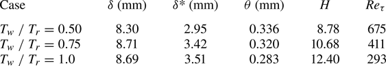
The streamwise position x_ref = −70 mm is selected as the reference position where the turbulent boundary layer is fully developed. Table 3 shows the boundary layer parameters of each case at x_ref, including the boundary layer thickness δ, displacement thickness δ*, momentum thickness θ and shape factor H. We enforce the value of δ to match closely at the reference station among simulations with different wall temperatures, which brings significant differences in the other parameters, especially the shape factor.

Table 3. Boundary layer parameters at x = −70 mm.

The total time for statistics collecting is more than $2{L_x}/{U_\infty }$ in each case, which means that the free-stream flow has passed through the whole streamwise computational domain at least twice. Because the boundary layer is in a laminar state during the initial period of simulations, the statistics are not collected during this period. We start collecting statistics after the flow has fully developed into turbulence (when the simulation time has approximately reached $3{L_x}/{U_\infty }$).

3. Results and discussion

3.1. Verification of results

Figure 3 shows the computational results of the mean (both time and spanwise averaged) wall pressure ${p_w}$ and skin friction coefficient which is defined as ${C_f} = {\tau _w}/({\rho _\infty }U_\infty ^{\; 2}/2)$, where ${\tau _w}$ is the wall shear stress. Here, δ is used to normalise the abscissa in the corresponding case. The results show that the mean ${p_w}$ and ${C_f}$ near the corner in the coarse meshes are almost the same as those in the fine meshes, indicating that the computational results are independent of the grid size at this grid resolution. As mentioned in § 2.2, the spanwise computational domain changes from 13.5 to 32 mm when ${T_w}/{T_r}$ changes from 0.50 to 1.0. To ensure that the computational domain is reasonable, we examine the two-point correlation coefficients of the three components of velocity at x = −70 mm and y ⁺ = 50 in each case, as shown in figure 4. Here, C_uu, C_vv and C_ww represent the two-point correlation coefficients of the streamwise, normal and spanwise velocities, respectively; r_z represents the distance between the two points. The results show the correlation of velocity approaching zero when ${r_z} > 0.2{L_z}$ and verify that the spanwise computational domain is sufficient to reflect the spanwise variation of turbulence in each case.

Figure 3. Streamwise distributions of the mean (a–c) wall pressure and (d–f) skin friction coefficient near the corner in the cases of (a,d) ${T_w}/{T_r} = 0.50$, (b,e) ${T_w}/{T_r} = 0.75$ and (c,f) ${T_w}/{T_r} = 1.0$.

Figure 4. Two-point correlation coefficients of the three components of velocity at the reference position with y ⁺ = 50 in the cases of (a) ${T_w}/{T_r} = 0.50$, (b) ${T_w}/{T_r} = 0.75$ and (c) ${T_w}/{T_r} = 1.0$.

In the following analyses, the Reynolds average of the general variable ψ is defined as $\bar{\psi }$, and the fluctuation of ψ from the Reynolds averaging operation is defined as $\psi ^{\prime} = \psi - \bar{\psi }$; the Favre average of ψ is defined as $\tilde{\psi }$, and the fluctuation of ψ from the Favre averaging operation is defined as $\psi ^{\prime\prime} = \psi - \tilde{\psi }$. The van Driest transformed (van Driest 1951) mean streamwise velocity $\bar{u}_{VD}^ + $ is defined as follows:

(3.1)\begin{equation}\bar{u}_{VD}^{+ } = \int_0^{{{\bar{u}}^ + }} {\sqrt {\bar{\rho }/\; {{\bar{\rho }}_w}} \,\textrm{d}\; {{\bar{u}}^ + }} ,\end{equation}

where ${\rho _w}$ is the density on the wall. Figure 5(a) shows the profiles of $\bar{u}_{VD}^{+ }$ at x_ref. Under different wall temperature conditions, $\bar{u}_{VD}^{+ }$ follows the log law:

(3.2)\begin{equation}\bar{u}_{VD}^{ + } = \frac{1}{\kappa }\,\textrm{ln}\,{y^ + } + C.\end{equation}

In the incompressible flow, the slope 1/κ and intercept C are approximately 2.44 and 5.1, respectively. In the present cases, the slopes are close to that in the incompressible boundary layer, while the intercepts are higher, ranging from 5.6 to 6.0. The higher intercepts were also shown in other studies on hypersonic turbulent boundary layers, such as C ranging from 5.2 to 6.0 at Mach 5 (Duan et al. 2010) and C = 5.9 at Mach 7.2 (Priebe & Martín 2021). The van Driest transformation only applies to the flow at a medium or low Mach number (van Driest 1951), which might cause a higher intercept in hypersonic conditions. In addition, the difference in the log law indicates that the intercept is more sensitive than the slope when the wall temperature changes. In addition to the log-law layer, the wall temperature also influences the viscous sublayer. As the wall temperature decreases, $\bar{u}_{VD}^{ + }$ deviates from the linear relation ($\bar{u}_{VD}^{ + } = {y^ + }$) at a position closer to the wall. At a lower wall temperature, the larger gradient in velocity and density makes the relation $\mu \partial u/\partial y = {\tau _w}$ unable to be integrated to get $\bar{u}_{VD}^{ + } = {y^ + }$ away from the wall (Duan et al. 2010). Therefore, under the condition of an adiabatic wall, the van Driest transformation is more applicable.

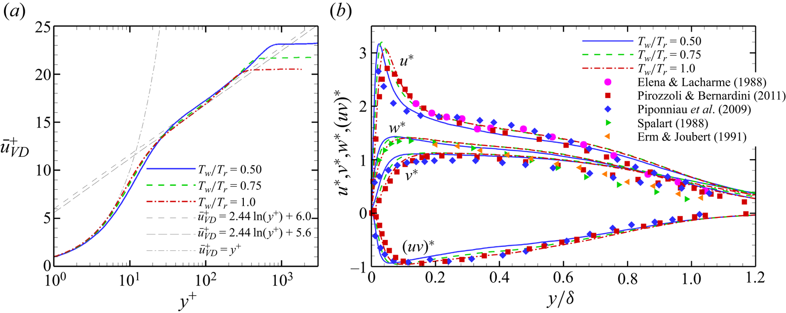
Figure 5. Profiles of (a) the van Driest transformed mean velocity and (b) velocity fluctuations at x_ref.

To take account of the effect of compressibility, we use the density-scaled velocity fluctuation (Pirozzoli & Bernardini 2011) as follows:

(3.3a,b)\begin{equation}u_i^\ast = \frac{{\sqrt {\bar{\rho }/{{\bar{\rho }}_w}} }}{{{u_\tau }}}\sqrt {\overline {u^{\prime 2}_i}} ,\quad {({u_i}{u_j})^\ast } = \frac{{\bar{\rho }/{{\bar{\rho }}_w}}}{{u_\tau ^2}}\overline {{u^{\prime}_i}{u^{\prime}_j}} ,\end{equation}

where ${u_\tau }$ is the friction velocity, defined as ${u_\tau } = \sqrt {{\tau _w}/\; {\rho _w}} $. Figure 5(b) compares the transformed velocity fluctuations with those of other studies (Elena & Lacharme 1988; Spalart 1988; Erm & Joubert 1991; Piponniau et al. 2009; Pirozzoli & Bernardini 2011), including incompressible flow or compressible flow at lower Mach numbers. With decreasing wall temperature, the position of the peak velocity fluctuation becomes closer to the wall, consistent with the study of Duan et al. (2010). According to the research of Pirozzoli & Bernardini (2011) and Spalart (1988), the difference in Re_θ might be the cause of this phenomenon.

Figure 6(a) compares the relations of mean temperature and streamwise velocity at different wall temperatures, where Walz's relation (Walz 1969) is given as follows:

(3.4)\begin{equation}\frac{{\bar{T}}}{{{{\bar{T}}_\infty }}} = \frac{{{{\bar{T}}_w}}}{{{{\bar{T}}_\infty }}} + \frac{{{{\bar{T}}_r} - {{\bar{T}}_w}}}{{{{\bar{T}}_\infty }}}\left( {\frac{{\bar{u}}}{{{{\bar{u}}_\infty }}}} \right) + \frac{{{{\bar{T}}_\infty } - {{\bar{T}}_r}}}{{{{\bar{T}}_\infty }}}{\left( {\frac{{\bar{u}}}{{{{\bar{u}}_\infty }}}} \right)^2}.\end{equation}

Walz's relation is a classic equation for boundary layers without a pressure gradient under adiabatic wall condition. When the wall temperature is closer to the recovery temperature, the difference between the temperature‒velocity relation and Walz's relation is smaller. In addition, the modified relation of Duan & Martin (2011) and the generalised Reynolds analogy relation of Zhang et al. (2014) are also compared in figure 6(a), these two relations are applicable to a non-adiabatic wall. The relation of Duan & Martin (2011) is as follows:

(3.5)\begin{align}\frac{{\bar{T}}}{{{{\bar{T}}_\infty }}} = \frac{{{{\bar{T}}_w}}}{{{{\bar{T}}_\infty }}} + 0.8259\frac{{{{\bar{T}}_r} - {{\bar{T}}_w}}}{{{{\bar{T}}_\infty }}}\left( {\frac{{\bar{u}}}{{{{\bar{u}}_\infty }}}} \right) + \left( {\frac{{{{\bar{T}}_\infty } - {{\bar{T}}_r}}}{{{{\bar{T}}_\infty }}} + 0.1741\frac{{{{\bar{T}}_r} - {{\bar{T}}_w}}}{{{{\bar{T}}_\infty }}}} \right){\left( {\frac{{\bar{u}}}{{{{\bar{u}}_\infty }}}} \right)^2}.\end{align}

The relation of Zhang et al. (2014) is as follows:

(3.6)\begin{equation}\frac{{\bar{T}}}{{{{\bar{T}}_\infty }}} = \frac{{{{\bar{T}}_w}}}{{{{\bar{T}}_\infty }}} + \frac{{{{\bar{T}}_{rg}} - {{\bar{T}}_w}}}{{{{\bar{T}}_\infty }}}\left( {\frac{{\bar{u}}}{{{{\bar{u}}_\infty }}}} \right) + \frac{{{{\bar{T}}_\infty } - {{\bar{T}}_{rg}}}}{{{{\bar{T}}_\infty }}}{\left( {\frac{{\bar{u}}}{{{{\bar{u}}_\infty }}}} \right)^2},\end{equation}

where ${\bar{T}_{rg}} = {\bar{T}_\infty } + r\bar{u}_\infty ^2/(2{C_p})$, ${r_g} = 2{C_p}({\bar{T}_w} - {\bar{T}_\infty })/\bar{u}_\infty ^2 - 2\,Pr\,{\bar{q}_w}/({\bar{u}_\infty }{\bar{\tau }_w})$; ${C_p}$ is the specific heat at constant pressure; ${q_w}$ is the heat flux. Because (3.5) and (3.6) are equivalent to (3.4) under the adiabatic wall condition, the results of these two equations at ${T_w}/{T_r} = 1.0$ are not included in figure 6(a). The temperature‒velocity curves of the present simulations match well with the modified relation of Duan & Martin (2011) and the generalised Reynolds analogy relation of Zhang et al. (2014). In addition, the temperature near the boundary layer edge diverges from Walz's relation in the case of ${T_w}/{T_r} = 1.0$. This is because this relation cannot well describe the overshoot of the total temperature profile in the outer region (Smits & Dussauge 1996). This overshoot is shown in figure 6(b), where T ₀ is the total temperature. At ${T_w}/{T_r} = 1.0$, T ₀ reaches the maximum (1.02 T _0∞) near in the outer region of the boundary layer. The overshoot is an inevitable result under adiabatic wall condition because the value of the total enthalpy equation integrated in the boundary layer is 0 and h ₀ is less than h _0∞ near the wall (h ₀ is the total enthalpy). Because Walz gave an approximation of the integration of the enthalpy equation, the error with the true enthalpy value gradually accumulates near the edge of the boundary layer, resulting in a certain difference between the DNS results and Walz's relation (Walz 1969).

Figure 6. Temperature‒velocity relations and total temperature profiles at x_ref.

The turbulence kinetic energy (TKE) is defined as $\tilde{k} = {\textstyle{1 \over 2}}\overline {\rho {{u^{\prime\prime}_i}}{{u^{\prime\prime}_i}}} /\bar{\rho }$, and the TKE budget equation is as follows:

(3.7)\begin{equation}\frac{{\partial (\bar{\rho }\tilde{k})}}{{\partial t}} + \widetilde {{u_i}}\frac{{\partial (\bar{\rho }\tilde{k})}}{{\partial {x_i}}} = {P_k} + {T_k} + \varPi + D + \varepsilon + {M_k},\end{equation}

where

(3.8)\begin{gather}{P_k} = - \overline {\rho {{u^{\prime\prime}_i}}{{u^{\prime\prime}_j}}} \frac{{\partial \widetilde {{u_i}}}}{{\partial {x_j}}},\end{gather}

(3.9)\begin{gather}{T_k} = - \frac{1}{2}\frac{\partial }{{\partial {x_j}}}\overline {\rho {{u^{\prime\prime}_i}}{{u^{\prime\prime}_i}}{{u^{\prime\prime}_j}}} ,\end{gather}

(3.10)\begin{gather}\varPi = {\varPi _t} + {\varPi _d} = - \frac{\partial }{{\partial {x_i}}}\overline {p^{\prime}{{u^{\prime\prime}_i}}} + \overline {p^{\prime}\frac{{\partial {{u^{\prime\prime}_i}}}}{{\partial {x_i}}}} ,\end{gather}

(3.11)\begin{gather}D = \frac{\partial }{{\partial {x_i}}}\overline {{{\tau ^{\prime}_{ij}}}{{u^{\prime\prime}_i}}} ,\end{gather}

(3.12)\begin{gather}\varepsilon = - \overline {{{\tau ^{\prime}_{ij}}}\frac{{\partial {{u^{\prime\prime}_i}}}}{{\partial {x_j}}}} ,\end{gather}

(3.13)\begin{gather}{M_k} = - {u^{\prime\prime}_i}\frac{{\partial \bar{p}}}{{\partial {x_i}}} + {u^{\prime\prime}_i}\frac{{\partial \overline {{\tau _{ij}}} }}{{\partial {x_j}}}-\bar{\rho }\tilde{k}\frac{{\partial \widetilde {{u_i}}}}{{\partial {x_i}}},\end{gather}

(3.14)\begin{gather}S = {P_k} + {T_k} + \varPi + D + \varepsilon + {M_k}.\end{gather}

In (3.7), $\; {P_k}$ is the TKE production term; $\; {T_k}$ is the turbulence transport term; $\varPi$ is the pressure term, including the pressure diffusion ${\varPi _t}$ and pressure dilation ${\varPi _d}$; D is the viscous diffusion term; ε is the viscous dissipation term; ${M_k}$ is the term due to the compressibility; S is the sum of all TKE budget terms. We use the semilocal scaling (Huang, Coleman & Bradshaw 1995) to normalise the budget terms by $\bar{\rho }(y)u_\tau ^{{\ast} 3}/y_\tau ^\ast $ and the normal coordinate by $y_\tau ^\ast $, where $u_\tau ^\ast = \sqrt {{\tau _w}/\bar{\rho }(y)} $ and $y_\tau ^\ast = \bar{\mu }(y)/(\bar{\rho }(y)u_\tau ^\ast )$. Figure 7(a−f) shows the profiles of these terms under each wall condition and compares the present results with those of the hypersonic turbulent boundary layer ‘M5T5’ in the research of Duan et al. (2010). Figure 7(g) indicates that the TKE budget terms are balanced. The results confirm the applicability of the semilocal scaling in hypersonic boundary layers and further verify the present DNS results.

Figure 7. Profiles of (a) TKE production, (b) turbulence transport, (c) pressure diffusion, (d) pressure dilation, (e) viscous diffusion, (f) viscous dissipation terms and (g) sum of all TKE budget terms at x_ref.

3.2. Flow structure

Figure 8 shows the instantaneous skin friction coefficient of each case. As the wall temperature increases, $R{e_\theta }$ and $R{e_\tau }$ decrease, leading to an increase in the inner scale of the turbulent boundary layer. As a result, the streamwise streak structure in the flat-plate region seems thinner at a lower wall temperature. Figure 9 shows the spanwise distributions of the instantaneous skin friction coefficient at the reference position, where $\overline {C_f^{\; z}}$ is the spanwise averaged instantaneous skin friction coefficient at the reference position, and the dashed lines mean ${C_f} - \overline {C_f^{\; z}} = 0$. The numbers of zero points of ${C_f} - \overline {C_f^{\; z}} $ are 22, 34 and 26 in the cases of ${T_w}/{T_r} = 0.5$, 0.75 and 1.0, respectively. If it is believed that there is a high-speed or low-speed streak between every two zero points, then the numbers of high-speed or low-speed streaks are 11, 17 and 13 in the corresponding cases, respectively. According to the width of the spanwise domain, it can be obtained that the averaged widths of each streak are 0.148, 0.203 and 0.283 δ in the cases of ${T_w}/{T_r} = 0.5$, 0.75 and 1.0, respectively. It is noteworthy that the wall units are 1.48 × 10⁻³, 2.43 × 10⁻³ and 3.41 × 10⁻³ δ in the cases of ${T_w}/{T_r} = 0.5$, 0.75 and 1.0, respectively. Therefore, the average width of each streak is close to 100 times of the wall unit in each case, which conforms to the description of the coherent structures of Marusic et al. (2010). Though it is not very precise to estimate the width of streaks according to the instantaneous skin friction coefficient, the main result is very clear that the streak structure of the turbulent boundary layer is thinner at a lower wall temperature, as appears in the research of Duan et al. (2010).

Figure 8. Contours of the instantaneous skin friction coefficient in the cases of (a) ${T_w}/{T_r} = 0.50$, (b) ${T_w}/{T_r} = 0.75$ and (c) ${T_w}/{T_r} = 1.0$.

Figure 9. Spanwise distributions of the instantaneous skin friction coefficient at x_ref in the cases of (a) ${T_w}/{T_r} = 0.50$, (b) ${T_w}/{T_r} = 0.75$ and (c) ${T_w}/{T_r} = 1.0$.

Figure 10 shows the instantaneous structures of the vortex visualised by the iso-surfaces of the Q-criterion (Jeong & Hussain 1995). In the flat-plate region, the streamwise vortices are dominant near the wall. In the separation region, the streamwise vortices disappear and are replaced by some broken separated vortices. Considering the reappearing streamwise streak structure in figure 7, it can be inferred that streamwise vortices appear again on the ramp downstream of the reattachment, though the iso-surfaces of the Q = 0.1 might not clearly show these streamwise vortices in all cases. However, these reappearing streamwise vortices in the reattached boundary layer are much smaller than their upstream counterparts, as shown in figure 7. In addition, the reattached boundary layer is much thinner than the upstream boundary layer, as shown by the isoline of mean vorticity $\bar{\omega }$ in figure 11. The thickness of the reattached boundary layer cannot be defined according to 0.99 U_∞ as the upstream. The vorticity reflects the shear in the flow field to some extent, which is related to the properties of the boundary layer. Therefore, we show the boundary layer thickness qualitatively by vorticity (Liu, Zhang & Wang 2018). In figure 11, to ensure the thickness defined by 0.99 U_∞ is equal to that marked by the isoline of $\bar{\omega }$, the vorticity ${\omega _{ref}}$ at the position with the coordinates (x, y) = (x_ref, δ) is selected as the reference in each case. Thus, the isoline of vorticity $\bar{\omega } = {\omega _{ref}}$ roughly reflects the outer edge of the boundary layer if the isoline near the shock wave is not considered. The much thinner reattached boundary layer means the normal gradient of velocity is much greater than the upstream, which brings a greater $R{e_\tau }$ and a smaller inner scale of the boundary layer. Therefore, the scale of the streamwise vortices downstream of the reattachment is smaller than their upstream counterparts.

Figure 10. Iso-surfaces of instantaneous Q = 0.1 coloured by the streamwise velocity in the cases of (a) ${T_w}/{T_r} = 0.50$, (b) ${T_w}/{T_r} = 0.75$ and (c) ${T_w}/{T_r} = 1.0$. Each case contains three locally enlarged subgraphs, corresponding to the flat-plate boundary layer, separation bubble and reattached boundary layer, respectively.

Figure 11. Contours of the mean vorticity in the x–y plane in the cases of (a,d) ${T_w}/{T_r} = 0.50$, (b) ${T_w}/{T_r} = 0.75$ and (c) ${T_w}/{T_r} = 1.0$. The green dashed line in each case is the isoline of $\bar{\omega } = {\omega _{ref}}$, where ${\omega _{ref}}$ is the vorticity at the position with the coordinates (x, y) = (x_ref, δ).

Figure 12 shows the mean streamwise velocity and streamlines near the corner. The separation bubble is characterised as a closed recirculation flow and its size significantly increases with the wall heating, as found in the earlier research (Spaid & Frishett 1972; Jaunet et al. 2014; Bernardini et al. 2016; Zhu et al. 2017). Inside the boundary layer, the momentum of fluids gradually decreases from the outer edge of the boundary layer towards the wall, and the separation occurs when the near-wall fluid cannot resist the adverse pressure gradient caused by the shock wave. Therefore, the differences in the momentum of the boundary layer might be an important factor leading to the variations in separation bubbles. The wall pressure is almost constant in the zero-pressure-gradient boundary layers, so the density of the near-wall fluid decreases when the wall temperature increases according to the ideal gas equation, as shown in figure 13(a). In addition, according to Sutherland's relation, the viscosity of near-wall fluid increases with wall temperature. The differences in the density and viscosity lead to the difference in the near-wall velocity profile and $R{e_\tau }$. Figure 13(b) shows that when the wall temperature decreases, the velocity profile becomes fuller, especially in the viscous sublayer. The greater density and velocity caused by wall cooling means that the near-wall fluid has greater momentum, as shown in figure 13(c). Therefore, the ability of the boundary layer to resist the adverse pressure gradient is stronger at a lower wall temperature, leading to a smaller separation bubble.

Figure 12. Contours of the mean streamwise velocity and streamlines in the x–y plane in the cases of (a,d) ${T_w}/{T_r} = 0.50$, (b) ${T_w}/{T_r} = 0.75$ and (c) ${T_w}/{T_r} = 1.0$, where panel (d) is the locally enlarged view of panel (a).

Figure 13. Profiles of the mean (a) density, (b) velocity and (c) momentum density at x_ref.

In STBLIs, turbulence amplification is a common and important phenomenon. As shown in figure 14, the TKE significantly increases in the interaction region, especially between the main flow and the separated flow. Two extreme values of TKE appear at the positions where the flow begins to separate and reattach. The upstream extreme value is mainly related to the speed reduction of the mean flow with streamwise velocity fluctuations; the strong turbulence in the downstream part is caused by the shear layer between the main flow and the separated flow (Fang et al. 2020). In addition, a larger separation bubble brings a larger flow deceleration region and a longer shear layer. Therefore, the region with a significantly strengthened TKE expands with the larger separation bubble caused by the higher wall temperature.

Figure 14. Contours of the turbulence kinetic energy in the x–y plane in the cases of (a) ${T_w}/{T_r} = 0.50$, (b) ${T_w}/{T_r} = 0.75$ and (c) ${T_w}/{T_r} = 1.0$.

Figure 15(a) shows the mean skin friction coefficient along the streamwise direction at different wall temperatures. Interestingly, near the corner (x = 0), the extreme value of C_f is greater than zero, which indicates that there is a much smaller separation bubble at the corner. This small separation bubble is induced by the counter flow at the bottom of the larger separation bubble. Figure 12(d) is the locally enlarged view of the corner in figure 12(a). In figure 12(d), the streamlines of recirculation indicate the small separation bubble, and the streamlines outside the small separation bubble indicate the counter flow at the bottom of the larger separation bubble. The rotation direction of the small separation bubble is opposite to that of the large separation bubble (the bubble in figure 12a), and the size of the former is two orders of magnitude smaller than the latter. In the following discussion, the description of the separation is only for the large separation bubble.

Figure 15. Streamwise distributions of the mean (a) skin friction coefficient and (b) wall pressure at different wall temperatures.

To analyse the quantitative effects of the wall temperature on the length of the separation, we define the upstream and downstream positions with C_f = 0 as the separation position x_s and reattachment position x_r, respectively. In addition, the streamwise position where the wall pressure begins to rise is defined as the interaction origin x ₀. In the present research, x ₀ corresponds to the position with $({p_w} - {p_{ref}})/{p_{ref}} = 0.01$, where ${p_{ref}}$ is the value of ${p_w}$ at x_ref. The values of x ₀, x_s and L are given in table 4.

Table 4. Locations of some special points.

Figure 15(b) shows the mean wall pressure distribution along the streamwise direction. As the wall temperature increases, the position of the interaction origin moves upstream, and the pressure plateau region becomes longer accordingly. In STBLIs, a pressure plateau is generally regarded as an area where the pressure changes slowly or remains almost unchanged between the two areas with relatively severe pressure increase. To quantitatively describe the pressure plateau, we consider defining a pressure plateau as an area where the pressure rise rate $\partial ({p_w}/{p_\infty })/\partial (x/\delta ) < 1$ between two areas with $\partial ({p_w}/{p_\infty })/\partial (x/\delta ) > 1$. The starting position x_{p 1} and ending positions x_{p 2} in each case are given in table 4. Unlike the starting position, the ending position of the pressure plateau seems insensitive when the wall temperature changes. Defining the pressure at the ending position as the value of the pressure plateau, then the value of the pressure plateau shows the similar insensitivity (${p_w}/{p_\infty } = 4.63$, 4.46 and 4.55 when ${T_w}/{T_r} = 0.50$, 0.75 and 1.00, respectively). In addition, at the separation position, the wall pressure also exhibits no obvious changes when the wall temperature significantly changes (${p_w}/{p_\infty } = 1.54$, 1.50 and 1.54 at the separation position when ${T_w}/{T_r} = 0.50$, 0.75 and 1.00, respectively).

The free-interaction theory (FIT) proposed by Chapman, Kuehn & Larson (1958) is commonly used to predict the wall pressure at the separation point and the pressure plateau. In the FIT, the boundary-layer momentum equation on the wall and the relationship between pressure and flow direction are applied to obtain the pressure rise equation as follows:

(3.15)\begin{equation}\frac{{\; {p_w} - {p_{w0}}}}{{{q_\infty }}} = F({x^\ast })\sqrt {\frac{{2{C_{f0}}}}{{{{(M_\infty ^{\; 2} - 1)}^{1/2}}}}} ,\end{equation}

where ${q_\infty }$ is the dynamic pressure defined as ${q_\infty } = {\rho _\infty }U_\infty ^{\; 2}/2 = \gamma M_\infty ^{\; 2}{p_\infty }/2$; x* is defined as ${x^\ast } = (x - {x_0})/{L_{0s}}$; ${L_{0s}}$ is the streamwise length scale defined as ${L_{0s}} = {x_s} - {x_0}$; $F({x^\ast })$ is the correlation function for the wall pressure, which has constant values at the separation position and pressure plateau (Babinsky & Harvey 2011); ${p_{w0}}$ and ${C_{f0}}$ are the wall pressure and skin friction coefficient at the interaction origin, respectively. Notably, (3.15) is only applicable to the interaction onset (upstream of the pressure plateau), so the overall pressure rise cannot be predicted in this way. According to (3.15), the increase in the wall pressure at the separation position or the pressure plateau is only determined by ${C_{f0}}$ and ${M_\infty }$ (upstream boundary layer parameters) and is independent of the shock wave strength. Because ${M_\infty }$ is the same and the difference in ${C_{f0}}$ is small in different cases, the pressure increase at the separation position or pressure plateau is almost the same when the wall temperature changes.

3.3. Prediction of wall pressure distribution

According to the above analysis, the pressure increase at the separation position or pressure plateau conforms to the FIT when the wall temperature changes. However, it is still worth verifying whether the pressure increase process in the whole interaction onset region follows the FIT. This validation requires more data on STBLIs with wall temperature changing. Therefore, we conduct DNS of the turbulent boundary layers over a 24° compression ramp under three wall temperature conditions according to the research of Zhu et al. (2017). The parameters of these three cases are given in table 5, where the thickness of the turbulent boundary layers (x_ref = −50 mm), grid size and resolutions are basically consistent with those of Zhu et al. (2017).

Table 5. Parameters of the present DNS based on the cases of Zhu et al. (2017).

Figure 16 shows the profile of the mean velocity of the present DNS. The van Driest transformed mean streamwise velocity is basically consistent with the log law and the result of Zhu et al. (2017). It should be noted that the present results have a deviation of approximately 5 % in the wake region. One possible reason is that Zhu et al. (2017) used the fourth-order bandwidth-optimised WENO scheme (Wu & Martin 2007). As mentioned before, in the present DNS, we use the hybrid difference scheme, whose numerical accuracy is close to UDL7 when adopted in the turbulent boundary layers. Therefore, the numerical dissipation of the difference scheme in the present DNS is smaller than that in the research of Zhu et al. (2017), which probably leads to a slight deviation in the simulations of the turbulent boundary layers. Figure 17 shows the streamwise distributions of the mean skin friction coefficient and wall pressure. The positions of separation and reattachment are very close to those in the research of Zhu et al. (2017). These comparisons verify the reliability of the present DNS results.

Figure 16. Profiles of the van Driest transformed mean velocity at x_ref = −50 mm with M _∞ = 2.9.

Figure 17. Streamwise distributions of the mean (a) skin friction coefficient and (b) wall pressure at different wall temperatures with M _∞ = 2.9.

Substituting ${q_\infty } = \gamma M_\infty ^{\; 2}{p_\infty }/2$ into (3.15), then the following equation can be obtained:

(3.16)\begin{equation}F({x^\ast }) = \frac{{\; {p_w}({x^\ast }) - {p_{w0}}}}{{\; {p_\infty }}}\frac{1}{{\gamma M_\infty ^{\; 2}}}\sqrt {\frac{{2{{(M_\infty ^{\; 2} - 1)}^{1/2}}}}{{{C_{f0}}}}} .\end{equation}

Therefore, according to the distribution function of the wall pressure ${p_w}({x^\ast })$ in each case, the corresponding correlation function $F({x^\ast })$ can be obtained (see figure 18). It is worth mentioning that ${x^\ast } = 1$ corresponds to the separation position, according to the definition of ${x^\ast }$. Though these cases have significant differences in Mach number, Reynolds number, compression angle and wall temperature, F shows similarity upstream of the corner, especially when ${x^\ast } < 2.5$. Therefore, it can be considered that the pressure increase process in the interaction onset region follows the FIT under different wall thermal conditions, this result is consistent with the research of Volpiani, Bernardini & Larsson (2020). The deviation of F gradually increases downstream of the pressure plateau because the FIT only applies to the interaction onset. Specifically, the pressure increase at the corner and the downstream position is partly decided by the downstream conditions, such as the compression angle. In figure 18, the values of F at the corner are 5.55−5.82 and 6.79−7.05 at M _∞ = 2.9 and 6.0, respectively. In addition, because ${x_0}$ and ${L_{0s}} = {x_s} - {x_0}$ are selected as the origin and reference length scale of x*, there is a significant difference in the values of x* at the corner.

Figure 18. (a) Correlation function F plotted through ${x^\ast }$ and its detail view at (b) M _∞ = 2.9 and (c) M _∞ = 6.0. The black dashed lines indicate the corner positions.

To improve the applicability of the FIT, we modify the normalisation method of streamwise length. We use ${x_s}$ rather than ${x_0}$ as the origin of streamwise coordinate because the former has a more accurate definition. Accordingly, interaction length $L = {x_c} - {x_s}$ is used as the reference length scale, where ${x_c}$ is the corner position (${x_c} = 0$ in the present cases). Therefore, the new streamwise coordinate χ is defined as $\chi = (x - {x_s})/L$, and $\chi = 0$ and 1 correspond to the separation and corner positions, respectively. Then, (3.16) is rewritten as

(3.17)\begin{equation}F(\chi ) = \frac{{\; {p_w}(\chi ) - {p_{w0}}}}{{\; {p_\infty }}}\frac{1}{{\gamma M_\infty ^{\; 2}}}\sqrt {\frac{{2{{(M_\infty ^{\; 2} - 1)}^{1/2}}}}{{{C_{f0}}}}} .\end{equation}

Figure 19 shows the correlation function F plotted through χ. Comparing figures 18(a) and 19(a), the latter shows a better similarity upstream of the pressure plateau. If there is only a difference in wall temperature between different cases, i.e. free-stream parameters and corner angle remain unchanged, then the curves of F plotted through χ show a better similarity than those through x*, including downstream of the pressure plateau, as shown in figure 18(b,c). As mentioned before, the value of F at the corner is almost unchanged if the free-stream parameters and the corner angle do not change. Of course, this unchanged characteristic is based on the relatively large separation extent, and it means that this separation is strong enough to cause the pressure plateau. Therefore, using $\mathrm{\chi }$ as the streamwise coordinate actually adds a constraint to F, i.e. F maintains a similar value and growth trend around χ = 1. However, because the value of F changes obviously with free-stream parameters and the corner angle, F still shows obvious deviation at the pressure plateau and its downstream region with M _∞ = 2.9 and 6.0. This reflects the limitation of FIT. Therefore, using ${x_s}$ and L as the normalisation scale has its scope of application, i.e. there is only a difference in wall temperature between different cases. Figure 20 shows that the similarity of F is also valid according to the data of Volpiani et al. (2020). It should be noted that the cases of Volpiani et al. are impinging shock interactions at M _∞ = 5.0, so ${x_c}$ corresponds to the shock impingement point.

Figure 19. (a) Correlation function F plotted through χ and its detail view at (b) M _∞ = 2.9 and (c) M _∞ = 6.0. The black dashed lines indicate the corner positions.

Figure 20. Correlation function F plotted through χ based on the data of Volpiani et al. (2020).

Through the above analyses, the correlation function shows good consistency in different cases, indicating that the scaling of the pressure increase function is valid by introducing F and χ. Therefore, based on (3.17), a relationship of wall pressure distribution between different wall thermal conditions can be established:

(3.18)\begin{align}\frac{{\; {p_{w1}}(\chi ) - {{({p_{w1}})}_0}}}{{\; {p_{\infty 1}}}}\frac{1}{{\gamma M_{\infty 1}^{\; 2}}}\sqrt {\frac{{2{{(M_{\infty 1}^{\; 2} - 1)}^{1/2}}}}{{{C_{f01}}}}} = \frac{{\; {p_{w2}}(\chi ) - {{({p_{w2}})}_0}}}{{\; {p_{\infty 2}}}}\frac{1}{{\gamma M_{\infty 2}^{\; 2}}}\sqrt {\frac{{2{{(M_{\infty 2}^{\; 2} - 1)}^{1/2}}}}{{{C_{f 02}}}}} ,\end{align}

where the variables with the subscripts ‘1’ and ‘2’ represent the corresponding variables under two different wall temperature conditions. It should be noted that (3.18) is only valid when $\chi < 1$ according to the applicability of the FIT. Because the similarity of F is based on the same free-stream parameters and corner angles, i.e. ${p_{\infty 1}} = {p_{\infty 2}}$ and ${M_{\infty 1}} = {M_{\infty 2}}$, (3.18) is simplified as follows:

(3.19)\begin{equation}{p_{w2}}(\chi ) - {({p_{w2}})_0} = ({p_{w1}}(\chi ) - {({p_{w1}})_0})\left( {\frac{{{C_{f2}}}}{{{C_{f1}}}}} \right)_0^{1/2}.\end{equation}

According to the definition of $\mathrm{\chi }$, (3.19) can be rewritten as

(3.20)\begin{equation}{p_{w2}}\left( {\frac{{{x_2}}}{{{\delta_2}}}} \right) - {({p_{w2}})_0} = \left( {{p_{w1}}\left( {\frac{{{x_1}}}{{{\delta_1}}}} \right) - {{({p_{w1}})}_0}} \right)\left( {\frac{{{C_{f2}}}}{{{C_{f1}}}}} \right)_0^{1/2},\end{equation}

where the relationship $({x_1} - {x_{s1}})/{L_1} = ({x_2} - {x_{s2}})/{L_2}$ needs to be met, and this relationship can also be written as

(3.21)\begin{equation}({x_1} - {x_{c1}})/{L_1} = ({x_2} - {x_{c2}})/{L_2}.\end{equation}

Equations (3.20) and (3.21) mean that when the wall temperature changes, if the pressure distribution at a certain wall temperature is known, then the pressure distribution at another wall temperature can be predicted. However, in addition to the upstream parameters ${C_{f0}}$ and ${p_{w0}}$, this relationship also depends on interaction length L. Therefore, a relationship between the interaction length and wall temperature needs to be established before the prediction of the pressure distribution.

Zhu et al. (2017) proposed a semi-theoretical formula to describe the relation between the separation bubble length L_sr = x_r − x_s and wall temperature as follows when the free-stream parameters are close:

(3.22)\begin{equation}{L_{sr}}/\delta \propto {({T_w}/{T_r})^{0.85}}.\end{equation}

Though there is a slight difference in the definitions between L and L_sr, both indicate the separation length scale. In addition, Touré & Schülein (2023) proposed a formula to describe the interaction length as follows:

(3.23)\begin{equation}\left. {\begin{array}{@{}c@{}} {L = {L^\ast }{\delta^\ast }\dfrac{{\textrm{sin}(\beta - \varphi )}}{{\textrm{sin}\,\; \beta \,\textrm{sin}\,\; \varphi }},}\\ {{L^\ast } = 15.46{{(c_p^\ast )}^2} - 1.07{{(c_p^\ast )}^4},}\\ {c_p^\ast = {{\left( {\dfrac{{R{e_\delta }}}{{2 \times {{10}^5}}}} \right)}^{ - 0.27c_p^{1.41}}}{{\left( {\dfrac{{{T_w}}}{{{T_r}}}} \right)}^{0.15}}{c_p},} \end{array}} \right\}\end{equation}

where β is the shock inclination; $\varphi $ is the flow deflection angle; pressure coefficient ${c_p}$ is defined as $({p_{out}} - {p_\infty })/(\gamma M_\infty ^{\; 2}{p_\infty }/2)$; ${p_{out}}$ is the final pressure.

The coefficients in (3.22) and (3.23) are mainly fitted based on numerical and experimental data at medium or low Mach numbers. Because (3.22) only gives a proportional relationship of L_sr and ${T_w}$ rather than explicit expression, we select L_sr at ${T_w}/{T_r} = 0.50$ as the reference, and then the predicted length in the other two cases can be obtained. In addition, considering the difference in the definitions, L_sr in (3.22) is substituted with L to further check the applicability of this equation. Table 6 shows the actual lengths of the present DNS at M _∞ = 6.0 and the corresponding predicted lengths according to (3.22) and (3.23), where $L^{\prime}$ and ${L^{\prime}_{sr}}$ are the predicted lengths based on (3.22), and $L^{\prime\prime}$ are based on (3.23). The results show that the relative errors of the predicted lengths based on (3.22) are less than 5 %, indicating that (3.22) is applicable to the present hypersonic STBLIs. Compared with (3.22), the prediction performance of (3.23) is not good at ${T_w}/{T_r} = 0.75$ and 1.0, and the latter seems to underestimate the effects of the wall temperature. This might be caused by the differences in the datasets. The coefficient in (3.22) is fitted according to the data of compression ramp interactions, while the coefficients in (3.23) are mainly fitted based on impinging shock interaction datasets. Based on (3.22), we assume the relationship,

(3.24)\begin{equation}L/\delta \propto {({T_w}/{T_r})^n},\end{equation}

is still applicable when the free-stream parameters are close in compression ramp STBLIs. The value of n might be affected by free-stream conditions and corner angle, and it needs further validation based on more data. Substantially, based on the datasets of Zhu et al. (including their numerical data and the experimental data of Spaid & Frishett (1972)) and the present results, the value of n is probably close to 0.85 in compression ramp STBLIs with relatively large separation extent, i.e. n ~ 0.85.

Table 6. Actual and predicted lengths, where ‘/’ means such quantity is not applicable to the case of ${T_w}/{T_r} = 0.50$ as it is taken as the reference.

According to (3.24), (3.21) can be rewritten as

(3.25)\begin{equation}{x_1} = \frac{{{\delta _1}}}{{{\delta _2}}}{\left( {\frac{{{T_{w1}}}}{{{T_{w2}}}}} \right)^n}({x_2} - {x_{c2}}) + {x_{c1}}.\end{equation}

Substituting (3.25) into (3.21), the following relationship can be obtained:

(3.26)\begin{align}{p_{w2}}\left( {\frac{{{x_2}}}{{{\delta_2}}}} \right) - {({p_{w2}})_0} = \left( {{p_{w1}}\left( {\frac{{({x_2} - {x_{c2}})}}{{{\delta_2}}}{{\left( {\frac{{{T_{w1}}}}{{{T_{w2}}}}} \right)}^n} + \frac{{{x_{c1}}}}{{{\delta_1}}}} \right) - {{({p_{w1}})}_0}} \right)\left( {\frac{{{C_{f 2}}}}{{{C_{f 1}}}}} \right)_0^{1/2}.\end{align}

For convenience, replace the independent variables ${x_2}$ with x, i.e.

(3.27)\begin{equation}{p_{w2}}\left( {\frac{x}{{{\delta_2}}}} \right) = \left( {\frac{{{C_{f2}}}}{{{C_{f1}}}}} \right)_0^{1/2}\left( {{p_{w1}}\left( {\frac{{(x - {x_{c2}})}}{{{\delta_2}}}{{\left( {\frac{{{T_{w1}}}}{{{T_{w2}}}}} \right)}^n} + \frac{{{x_{c1}}}}{{{\delta_1}}}} \right) - {{({p_{w1}})}_0}} \right) + {({p_{w2}})_0}\textrm{,}\end{equation}

where n ~ 0.85 in the compression ramp STBLIs. Therefore, if ${p_{w1}}(x/{\delta _1})$ is known and the parameters of the boundary layer (including $\delta $, ${C_{f0\; }}$ and ${p_{w0}}$) at ${T_{w1}}$ and ${T_{w2}}$ are known as well, then ${p_{w2}}(x/{\delta _2})$ can be obtained. The applicability of (3.27) is based on three conditions: the cases at ${T_{w1}}$ and ${T_{w2}}$ have the same free-stream parameters and corner angles; the separation is strong enough to cause the pressure plateau; the independent variables $x < {x_c}$.

If the corner position ${x_c}$ is set as the origin of the streamwise coordinate, (3.27) can be simplified as

(3.28)\begin{equation}{p_{w2}}\left( {\frac{x}{{{\delta_2}}}} \right) = \left( {\frac{{{C_{f 2}}}}{{{C_{f 1}}}}} \right)_0^{1/2}\left( {{p_{w1}}\left( {\frac{x}{{{\delta_2}}}{{\left( {\frac{{{T_{w1}}}}{{{T_{w2}}}}} \right)}^n}} \right) - {{({p_{w1}})}_0}} \right) + {({p_{w2}})_0}.\end{equation}

Equation (3.28) means that the pressure rise function $\Delta {p_{w2}}(x/{\delta _2})$ can be obtained when the independent variable coordinate of $\Delta {p_{w1}}(x/{\delta _1})$ is scaled by ${\delta _2}/{\delta _1} {({T_{w2}}/{T_{w1}})^n}$ and the dependent variable coordinate is scaled by $({C_{f2}}/{C_{f1}})_0^{1/2}$, where $\Delta {p_w}(x/\delta ) = {p_w}(x/\delta ) - {p_{w0}}$.

To verify the applicability of the above deduction, we select the case of ${T_w}/{T_r} = 1.4$ at M _∞ = 2.9 as the reference (subscripts ‘1’ in (3.28)), and then the wall pressure distribution of the other two cases at M _∞ = 2.9 can be predicted by (3.28). Similarly, the case of ${T_w}/{T_r} = 0.50$ is the reference of the prediction at M _∞ = 6.0. Here, n is set to 0.85 in the prediction. Figure 21 shows that the prediction results are generally consistent with DNS when $x < 0$. However, due to the limitations of the FIT, the prediction error gradually increases when $x > 0$, especially at M _∞ = 6.0. It should be noted that the rule of separation at a high Reynolds number might differ from that at a low Reynolds number (Babinsky & Harvey 2011). In the present cases with Re_τ ranging from 160 to 675, the applicability of the prediction equation can be preliminarily confirmed. The applicability of this equation still needs further verification at other Reynolds numbers.

Figure 21. Prediction results of the mean wall pressure at (a) M _∞ = 2.9 and (b) M _∞ = 6.0 using (3.28).

3.4. Low-frequency unsteadiness phenomenon

In STBLIs, the separation shock wave foot moves back and forth in an area called the intermittent region at a frequency one to two orders of magnitude lower than the characteristic frequency of the upstream turbulent boundary layer. The characteristic frequency of the turbulent boundary layer is usually the same order of magnitude as the boundary-layer outer-scale frequency which is defined as ${U_\infty }/\delta $. Correspondingly, the characteristic frequency of the separation shock low-frequency motion is approximately 0.01–0.1 ${U_\infty }/\delta $. The analysis of the low-frequency unsteadiness requires that the total time span of sampling includes at least several periods of the low-frequency motion, so the flow field needs to develop for a very long time (advancing over one million time steps in the present cases). Because of the verified grid independence, the time evolution and sampling are conducted in the coarse mesh of each case to reduce the amount of computation.

In previous research on low-frequency unsteadiness, time is commonly normalised by $\delta /{U_\infty }$, and the Strouhal number $S{t_\delta } = f\delta /{U_\infty }$ is used to represent the dimensionless frequency accordingly, where f is the actual frequency. In the present research, we sample the wall pressure evolution with time in the middle x–y plane (z = L_z/2) at each wall temperature. The total sampling time of each case is more than 1000 $\delta /{U_\infty }$, and the time interval between two adjacent samples is approximately 0.058 $\delta /{U_\infty }$. Figure 22 shows the sampled data of the wall pressure at a station with the coordinates (x, y, z)/δ = (−4.39, 0, 3.68) in the case of ${T_w}/{T_r} = 1.0$. A Butterworth filter with a cutoff frequency of 0.02 ${U_\infty }/\delta $ is used to conduct low-pass filtering for the raw data to eliminate high-frequency pulsation. The low-pass filtered wall pressure has an obvious characteristic of low-frequency pulsation because this station is located in the intermittent region.

Figure 22. Evolution of the wall pressure at the station with the coordinates (x, y, z)/δ = (−4.39, 0, 3.68) in the case of ${T_w}/{T_r} = 1.0$.

Figure 23 shows the contour of the weighted power spectral density (WPSD) (Pasquariello, Hickel & Adams 2017) of the wall pressure in each case. The WPSD is defined as follows:

(3.29)\begin{equation}\textrm{WPSD}(f) = \frac{{f \times \textrm{PSD}(f)}}{{\displaystyle\int {\textrm{PSD}(f)\,\textrm{d}f} }},\end{equation}

where PSD is the power spectral density of the wall pressure, obtained through the fast Fourier transform (FFT). A region with obvious low-frequency energy appears in each case, and this low-frequency energy has a wide frequency domain. The dominant frequency $S{t_\delta }$ of the low-frequency motion is approximately 0.015–0.03. The intermittent region length ${L_i}$ is defined as the distance between the interaction origin and separation position (${L_i} = {L_{0s}}$), and the values of ${L_i}$ are 0.61, 0.74 and 1.07 $\delta $ in the cases of ${T_w}/{T_r} = 0.5$, 0.75 and 1.0, respectively. Accordingly, the Strouhal number defined in terms of the intermittent region length is $S{t_{{L_i}}} = f\,{L_i}/{U_\infty }$. The dominant frequency $S{t_{{L_i}}}$ of the low-frequency motion is approximately 0.016–0.022, which is close to the previous research results (Gonsalez & Dolling 1993). As the wall temperature rises, the energy of the low-frequency motion and the size of the intermittent region significantly increase, and the dominant frequency of the low-frequency motion decreases. Interestingly, the characteristic frequency upstream from the interaction region seems to rise as the wall temperature decreases. Although the outer scale (boundary layer thickness) at each wall temperature is very close, the inner scale significantly increases with the wall temperature, according to figures 8 and 9. In general, the scale and frequency are negatively correlated, so the characteristic frequency in the upstream turbulent boundary layer is higher at a lower wall temperature.

Figure 23. Contours of the wall pressure WPSD in the cases of (a) ${T_w}/{T_r} = 0.50$, (b) ${T_w}/{T_r} = 0.75$ and (c) ${T_w}/{T_r} = 1.0$.

To quantitively analyse the effect of the wall temperature on the low-frequency unsteadiness, we divide the PSD into the low-frequency part ($\lg (S{t_\delta }) \le - 1$) and mid-to-high-frequencies part ($\lg (S{t_\delta }) > - 1$). The PSD in the low-frequency part is integrated at each streamwise position to obtain the low-frequency energy proportion ${P_L}$:

(3.30)\begin{equation}{P_L} = \frac{{\displaystyle\int_{{f_{min}}}^{{f_L}} {\textrm{PSD}(f)\,\textrm{d}f} }}{{\displaystyle\int_{{f_{min}}}^{{f_{max}}} {\textrm{PSD}(f)\,\textrm{d}f} }},\end{equation}

where f_max is the maximum frequency resolved in the FFT (i.e. f_max is half of the sampling frequency); f_min is the minimum frequency resolved in the FFT when the number of discrete points is set to 4096 (i.e. f_min is 1/4096 of the sampling frequency); f_L is the corresponding frequency when $\lg (S{t_\delta }) = - 1$. Figure 24 shows the streamwise distributions of the low-frequency energy proportion at different wall temperatures. The peak of the low-frequency energy proportion appears between the interaction origin and separation position, and its value exceeds 0.5 in the case of ${T_w}/{T_r} = 0.75$ or 1.0. This means that the low-frequency motion is dominant in the intermittent region. The peak energy proportion of the low-frequency motion increases by approximately 28 %, and the size of the region with ${P_L} > 0.3$ increases by approximately 200 % as ${T_w}/{T_r}$ changes from 0.50 to 1.0. That is, reducing the wall temperature can significantly suppress low-frequency unsteadiness.

Figure 24. Streamwise distributions of the low-frequency energy proportion.

Apart from the low-frequency unsteadiness, the wall temperature also affects the recovery process of the flow characteristic frequency from the middle frequency ($\lg (S{t_\delta }) \approx - 0.5$) to the high frequency ($\lg (S{t_\delta }) \ge 0$). The mid-frequency motion in the separation region is related to the shear or convection oscillations between the main and separated flows. Downstream from the reattachment, the separated flow recovers to the boundary layer, so the changing process of the dominant frequency is connected to the reattachment process. The decrease in the wall temperature results in the reattachment position moving upstream, which means that the dominant frequency recovers to the high frequency in a shorter streamwise distance.

3.5. Mechanisms of low-frequency unsteadiness

Although there is no final conclusion on why low-frequency unsteadiness occurs in STBLIs (Clemens & Narayanaswamy 2014), it is usually considered that the driving mechanism of this phenomenon is related to the forcing by the upstream turbulent boundary layer or the intrinsic unsteadiness of the downstream separation flow. To further investigate the impact of upstream and downstream mechanisms on low-frequency unsteadiness, we select nine stations along the streamwise direction in the middle x–y plane at each wall temperature, as shown in table 7. According to figure 24, we select the position with the maximum low-frequency energy proportion as the reference station (Station 5), with four stations distributed upstream (Stations 1–4) and four stations distributed downstream (Stations 6–9). These nine stations are evenly spaced, and Station 1 is located in the turbulent boundary layer without interactions. The correlation coefficients with delay time (τ) between the wall pressure at each station and that at Station 5 are shown in figure 25, where the correlation coefficient with delay time between general variables α and β is defined as

(3.31)\begin{equation}{R_{\alpha ,\beta }}(\tau ) = \frac{{\sum {[(\alpha (t + \tau ) - \bar{\alpha }) (\beta (t) - \bar{\beta })]} }}{{\sqrt {\sum {\sum {{(\alpha (t + \tau ) - \bar{\alpha })}^2}} } \sqrt {\sum {{{(\beta (t) - \bar{\beta })}^2}} } }}.\end{equation}

It is noteworthy that the above equation reflects the correlation between β and α which lags behind β for a delay time τ. In other words, ${R_{\alpha ,\beta }} \ne 0$ means that when the variable α responds to the variable β, it has been a time τ since the event reflected by β occurs. Therefore, if ${R_{\alpha ,\beta }} \ne 0$ and τ > 0, then there is a certain correlation between α after a certain time τ and β. Conversely, if ${R_{\alpha ,\beta }} \ne 0$ and τ < 0, then there is a certain correlation between α a certain time $|\mathrm{\tau }|$ ago and β. In figure 25, the wall pressure at Station 5 can be regarded as β in (3.31), and the wall pressure at a certain station can be regarded as α.

Table 7. Streamwise coordinates ($x/\delta $) of each station.

Figure 25. Correlation coefficients with delay time between the wall pressure at each station and that at Station 5 in the cases of (a,b) ${T_w}/{T_r} = 0.50$, (c,d) ${T_w}/{T_r} = 0.75$ and (e,f) ${T_w}/{T_r} = 1.0$.

Through the analysis of correlations, we want to explain how the upstream and downstream fluctuations impact the low-frequency region and which one of the upstream and downstream mechanisms dominates in the low-frequency motions. Before the discussion, it should be clarified that the low-frequency motion and low-frequency region are two different concepts. In the low-frequency region, there exists both low-frequency motion and mid-to-high-frequencies motion, though the former is the dominant. Therefore, figure 25 reflects the correlations between the upstream or downstream stations and the low-frequency region (Station 5) rather than low-frequency motion.

Figure 25(a,c,e) shows the correlations between Stations 1–4 and Station 5 at different wall temperatures. There is a prominent peak value in each correlation curve, and the delay time corresponding to the peak (which we called the characteristic delay time) is negative. As the distance from Station 5 increases, the peak value of the correlation gradually decreases, and the absolute value of the characteristic delay time increases. Similar phenomena also appear in the correlation curve between Stations 6–9 and Station 5, although the characteristic delay times are all positive, as shown in figure 25(b,d,f). The negative characteristic delay time at the position upstream from Station 5 means that the upstream pressure fluctuations occur earlier than the corresponding pressure fluctuations at the position with significant low-frequency unsteadiness. Therefore, the upstream disturbance might be one of the factors that affect the downstream low-frequency region. Interestingly, this upstream effect is also manifested in the positive characteristic delay time at the position downstream from Station 5, although the mean velocity near the wall is negative (i.e. the mean flow developing from the downstream to the upstream) at some downstream stations. Another noteworthy phenomenon is that there is a lower peak value in the correlation curve of some stations in addition to the most prominent peak value. These two peaks are particularly evident at Stations 4 and 6. To distinguish between these two peaks, we refer to the most prominent peak and the lower peak as the first peak and the second peak, respectively. The delay time of the second peak is positive at the upstream stations and negative at the downstream stations, in contrast to that of the first peak. Therefore, the second peak reflects that the downstream pressure changes occur earlier than the upstream pressure changes, which is a manifestation of downstream impact.

The appearances of the first and second peaks indicate the competitive upstream and downstream impacts and the features of these two peaks can reflect the differences between the upstream and downstream impacts.

First, the first peak appears in the correlation curve of each station, while the second peak is not obvious in the correlation curve of Stations 1 and 2. The absent second peaks at the upstream stations indicate that the downstream effect only appears in the interaction region, which is different from the upstream effect that appears in both the undisturbed boundary layer and interaction region. In the hypersonic boundary layer, the perturbations propagating at the speed of sound can only transmit from upstream to downstream. In the interaction region, the boundary layer is separated, and the subsonic circulating flow appears in the separation bubble, which means that the perturbations can propagate both upstream and downstream. Therefore, the scope of the downstream effect is limited, while the upstream effect can exist at all streamwise positions unless there is steady supersonic backward flow. It should be noted that the terms ‘upstream’ and ‘downstream’ are mentioned from the perspective of the whole flow field and are not based on the direction of local flow. In addition, although the first peak appears at all stations, the first peak is less prominent at the downstream stations compared with the upstream stations. The comparison of the first peak at Stations 1 and 9 demonstrates this feature. Stations 1−4 are located upstream from the separation region, where the near-wall mean flow is still a forward flow. Consequently, the fluctuations from the upstream stations are naturally brought to Station 5 by the mean flow. In contrast, Stations 6−9 are located near the separation line, where the velocity of the mean flow sharply decreases, and even the backward flow appears. It means that the fluctuations from Station 5 are hardly propagated to the downstream stations through the near-wall mean flow. Therefore, the upstream impact is less significant at the downstream stations, which is the reason for the weakness of the first peak here.

Second, the span of the delay time corresponding to the first peak is narrower than that corresponding to the second peak; that is, the first peak appears steeper than the second peak. Taking the correlation curve of Station 6 in figure 25(d) as an example, as the delay time deviates from the characteristic times of these two peaks, the value of the correlation drops rapidly near the first peak but slowly near the second peak. This phenomenon indicates that the downstream pressure response to the upstream pressure change is direct and rapid, but the upstream needs a longer time span in response to the downstream pressure change. In other words, the upstream can only affect the downstream at a certain time after the appearance of fluctuation, while the downstream fluctuation can affect the upstream at a longer period.

The above analysis indicates that both the upstream and downstream have noticeable impacts on the fluctuations in the low-frequency region. However, even in the low-frequency region, there are still some high-frequency fluctuations that cannot be ignored. To further investigate the impact of upstream and downstream mechanisms on the low-frequency fluctuations rather than the high-frequency fluctuations, we conducted low-pass filtering on the raw pressure pulsation signals of Station 5. The cutoff frequency of the low-pass filter is 0.1 ${U_\infty }/\delta $. Then we obtain the correlation coefficients with the delay time between the raw signals at Stations 1–9 and the filtered signals (low-frequency signals) at Station 5 according to (3.31), as shown in figure 26. Compared with figure 25, figure 26 shows that the first peak disappears, while the second peak is almost unaffected by filtering. As mentioned before, the first and second peaks reflect the influence of upstream and downstream signals on the low-frequency region, respectively. This indicates that the pulsating signals from upstream do not have a significant impact on the low-frequency signals at Station 5, that is, the downstream mechanism is the dominant factor causing low-frequency unsteadiness. Therefore, the first peak in figure 25 reflects the upstream impact on the high-frequency fluctuations in the low-frequency region. This conclusion, to some extent, can be inferred by the second difference between the upstream and downstream impacts in the previous analysis.

Figure 26. Correlation coefficients with delay time between the wall pressure at each station and the low-pass filtered wall pressure at Station 5 in the cases of (a,b) ${T_w}/{T_r} = 0.50$, (c,d) ${T_w}/{T_r} = 0.75$ and (e,f) ${T_w}/{T_r} = 1.0$.

Based on the above analysis of the causes of low-frequency unsteadiness, how the wall temperature affects low-frequency unsteadiness can be further discussed. As mentioned before, wall cooling can directly reduce the inner scale of the turbulent boundary layer and the size of the separation bubble. The wall temperature influences on the turbulent boundary layer and separation bubble correspond to upstream and downstream mechanisms of low-frequency unsteadiness, respectively. Therefore, the explanation for the influence of the wall temperature on the low-frequency unsteadiness is mainly weighted in the separating bubbles, as in some previous research (Thomas, Putnam & Chu 1994; Wu & Martin 2008; Touber & Sandham 2009). At a higher wall temperature, the separation bubble is larger, which means that its large-scale expansion or contraction is more visible, leading to a larger streamwise range for the separation shock oscillation. Therefore, a higher wall temperature can cause a larger intermittent region and stronger low-frequency unsteadiness. Moreover, a larger scale of the separation shock oscillation makes the period of this motion longer, leading to a lower dominant frequency of the low-frequency oscillation.

In addition, the turbulence structures of the upstream boundary layer have smaller scales and higher frequencies at a lower wall temperature. Consequently, when these turbulence structures flow into the interaction region, the fluctuations with smaller scales and higher frequencies are brought to the low-frequency region. It means that the low-frequency energy proportion will be diluted by more high-frequency energy, though the former is still dominant in the low-frequency region. That is to say, the wall cooling might reduce the low-frequency energy proportion by affecting the features of the upstream boundary layer. This process, to some extent, reflects the upstream mechanism. However, this is not the main factor of the suppressed low-frequency unsteadiness at a cold wall, considering that the upstream mechanism is not dominant in this phenomenon. The influence from upstream is indirect, meaning it does not directly weaken the low-frequency energy. This contrasts sharply with the downstream mechanism, in which the wall cooling directly weakens the strength of the low-frequency motion by reducing the size of the separation bubble.

4. Conclusion

In the present research, we conduct DNSs of STBLIs in a 34° compression ramp at M_∞ = 6 with three different wall temperatures ranging from ${T_w}/{T_r} = 0.50$ to ${T_w}/{T_r} = 1.0$. After verifying the grid independence and turbulent boundary layer profiles, we analyse the instantaneous and mean flow fields and the low-frequency unsteadiness. The main conclusions are summarised as follows.

1. (1) As the wall temperature rises, the inner scale of the turbulent boundary layer increases with $R{e_\tau }$ decreasing. In addition, cooling the wall can reduce the size of the separation bubble. This is because a colder wall contributes to fuller profiles of density and velocity in the turbulent boundary layer, leading to a greater momentum of the near-wall fluid to resist the separation. The wall pressure at the pressure plateau and the separation point is not sensitive to the change in the wall temperature.

2. (2) According to the FIT and the simulation data, the following equation is proposed to predict the wall pressure rise process upstream from the corner when the wall temperature changes:

   (4.1)\begin{align}{p_{w2}}\left( {\frac{x}{{{\delta_2}}}} \right) = \left( {\frac{{{C_{f 2}}}}{{{C_{f 1}}}}} \right)_0^{1/2}\left( {{p_{w1}}\left( {\frac{{(x - {x_{c2}})}}{{{\delta_2}}}{{\left( {\frac{{{T_{w1}}}}{{{T_{w2}}}}} \right)}^n} + \frac{{{x_{c1}}}}{{{\delta_1}}}} \right) - {{({p_{w1}})}_0}} \right) + {({p_{w2}})_0}.\end{align}

3. The applicability of this equation is based on three conditions: the cases at ${T_{w1}}$ and ${T_{w2}}$ have the same free-stream parameters and corner angles; the separation is strong enough to cause the pressure plateau; the independent variables $x < {x_c}$. The results predicted by this equation are generally consistent with those of the simulations (M_∞ = 2.9 and 6, Re_τ = 160−675).

4. (3) Cooling the wall can significantly suppress the low-frequency unsteadiness by reducing the energy of the low-frequency motions and narrowing its streamwise range. The analysis of the correlation between the upstream and downstream flows indicates that the low-frequency unsteadiness is mainly driven by the downstream mechanism. Therefore, the suppressed low-frequency unsteadiness is caused by the decreasing size of the separation bubble when the wall temperature decreases.