1. Introduction
Despite growth and globalization, which is expected to delay the age at first marriage; child marriage continues to exist even in the twenty-first century even though it robs millions of their childhood and violates their fundamental human rights. The adverse effects of child marriage for girls are often considered to be manifold as it not only affects these adolescent girls themselves but also has intergenerational effects on their children, affecting their educational attainment, health outcomes and overall human capital acquisition. According to the Indian Constitution, a marriage is considered a child marriage if either the age of the bride is below 18 or the age of the groom is less than 21 years as on the day of the marriage. Despite the prevalence of strict marriage laws in most countries, this practice is still prevalent in many developing countries such as India, where cultural traditions and social norms have taken an upper hand over legislative law and the mechanisms to implement these laws are inadequate due to weak institutions. In spite of various strict laws against child marriage like the Child Marriage Restrain Act of 1930 and the Prohibition of Child Marriage act of 2006 to forcefully prevent the incidence of child marriage, its incidence still stands at 27% in India [UNICEF (2017)], a decline of just 8% from 35% in 2007–08 (DLHS-3), making India home to the world's highest number of child brides. According to UNICEF (2014), 42% of global child brides live in South Asia and India alone accounts for one-third of total child brides worldwide. The practice of child marriage has declined only marginally over the decades and large variations in incidence of child marriage as well as average age at marriage still exist across different states and across districts within the same state [NFHS (2007)].
The major reasons often cited behind the existence of child marriage in the society are poverty, lack of education, awareness about the existing laws regarding child marriage and social pressure due to deep-rooted cultural norms [Maharia et al. (Reference Maharia, Maiti and Pakrashi2019)]. Certain societies attach strong cultural emphasis on female modesty and chastity and social stigma to having a young girl after puberty in their paternal house, while certain cultural and religious practices may be the prime reason for the backward castes. Early marriage is often perceived as a socially accepted strategy to ensure physical safety and safeguard the chastity of adolescent girls from adverse events such as rape, molestations and kidnaping, particularly if they reside in neighborhoods with high levels of sexual crimes against women [Desai and Andrist (Reference Desai and Andrist2010), Verma et al. (Reference Verma, Srinivasan, Mishra, Walia, Sharma, Weiss and Abrahamson2014), Maharia et al. (Reference Maharia, Maiti and Pakrashi2019)]. There also exists a premium on age in the marriage market in the context of dowry, which continues to be an integral part of the Indian marriage system, irrespective of religion and caste [Srinivasan and Lee (Reference Srinivasan and Lee2004)]. The value of dowry increases with the age of the bride [Chowdhury (Reference Chowdhury2010)] and so poor families are more likely to marry their girls early. Younger brides are also more likely to marry in a relatively rich household as matching in the marriage market is considered to be a multi-dimensional process, where households may be willing to trade off younger brides for some other desirable traits in the husbands and their families.
There are at least two channels via which early marriage of women may affect reproductive health and utilization of health facilities, particularly during pregnancy and delivery. The first channel is through a more direct autonomy-based disadvantage. Child brides due to their young age have less autonomy and limited voice in the household decision-making, which eventually affects their educational attainment thereafter, fertility preferences and healthcare choices. On the other hand, younger brides may receive comparatively better marriage prospects, which may eventually improve the overall health outcomes of women married off early by way of better resource provision. The effect of child marriage on reproductive health, fertility choices and utilization of other health facilities made available by the government, therefore depends on the relative strengths of these two effects, which work in opposite direction. The overall effect is therefore theoretically ambiguous and warrants a detailed empirical examination.
Using detailed data from the third round of the District Level Household Survey (also referred to as DLHS-3) conducted in India between 2007 and 2008, this paper examines the impact of child marriage of women on usage of modern family planning methods like male or female sterilization, birth control pills and condoms; and uptake of different healthcare facilities during pregnancy and delivery; such as registering their pregnancy, receiving antenatal care from a formal place and delivering at a government or private institution under the supervision of modern health personnel. For the purpose of analysis, we consider ever married women in the 15–49 age group and lay particular emphasis on women residing in the states of Uttar Pradesh and Bihar, two states with the highest incidence of child marriage and lowest average age at marriage (in years), and women belonging to the 20–24 age cohort has been focused. The main challenge, however, in using the standard ordinary least squares (OLS) method as the primary empirical strategy to identify the effect of child marriage on the variables of interest is that the results estimated using this approach cannot be interpreted as causal in nature.
In order to eliminate the endogeneity problem, inherent in estimating this effect due to the presence of confounding factors that may affect both age of the woman at the time of marriage and her choices, the instrumental variable (IV) approach has been adopted. Exogenous variation in rainfall at the district level has been used as an instrument for the incidence of child marriage in the household i.e. whether the respondent was married before she reached the legal age of marriage for girls. Together with the OLS estimates, the IV results give some weight to the fact that a direct effect is indeed there and the results can be interpreted as causal. The overall results presented in the paper suggest that women who marry early, i.e. before their 18th birthday are more likely to give birth before they turn 18 and experience loss of children. They are also less likely to use contraception currently and access modern health facilities during both pregnancy and childbirth. All these results confirm that the first autonomy effect dominates the resource effect resulting in a negative effect of child marriage of women on her reproductive health. The results, however, vary extensively based on the state of residence and the age of the woman.
The rest of the paper is organized as follows. Section 2 discusses the relevant literature and highlights the contribution of this paper to the literature. Section 3 outlines the empirical strategy, followed by a brief description of the data in Section 4. Section 5 discusses the regression results and provides checks to confirm the validity of the instrument used. Finally, conclusion of the paper has been drawn in Section 6.
2. Background and literature review
Several papers have shown that while parents may perceive substantial economic and non-economic gains from marrying off their daughter early [Verma et al. (Reference Verma, Srinivasan, Mishra, Walia, Sharma, Weiss and Abrahamson2014)] for reasons discussed earlier, there may exist several adverse effects that may arise from these young women being physically and psychologically more vulnerable than their older counterparts, who are more likely to be educated and less likely to be socially isolated. Young girls who marry early are more likely to have higher fertility rates due to inadequate contraceptive use, repeated childbirths in two years, failed pregnancies due to miscarriages, complicated pregnancies and deliveries and give birth to underweight babies [Raj et al. (Reference Raj, Saggurti, Balaiah and Silverman2009),] and are often married to significantly older men [UNICEF (2005)]. They are also more likely to have early and high-risk pregnancies, are at risk of contracting sexually transmitted diseases and have less control over their husband's resources [Black (Reference Black2001), Jejeebhoy and Bott (Reference Jejeebhoy and Bott2003), Jensen and Thornton (Reference Jensen and Thornton2003), Mathur et al. (Reference Mathur, Greene and Malhotra2003), Jain and Kurz (Reference Jain and Kurz2007), UNICEF (2009, 2011), Malhotra et al. (Reference Malhotra, Warner, McGonagle and Lee-Rife2011)].
Early marriage increases their likelihood of being a victim of domestic violence in their in-laws. Roychowdhury and Dhamija (Reference Roychowdhury and Dhamija2020) finds that delaying the marital age of women by a year reduces incidence of severe and less severe physical violence by 4 and 7 percentage points respectively using the IV strategy, whereby they instrument the age at marriage by age at menarche. Other studies have also shown an association between early marriage and domestic violence in developing countries such as Pakistan and Bangladesh [Nasrullah et al. (Reference Nasrullah, Zakar and Zakar2014), Yount et al. (Reference Yount, Crandall, Cheong, Osypuk, Bates, Naved and Schuler2016)].
Previous research has shown that women's early marriage not only limits their own educational attainment and human capital acquisition [Field and Ambrus (Reference Field and Ambrus2008)] and restricts their employment or economic advancement [Nanda et al. (Reference Nanda, Das, Singh and Negi2013)] but also influences the education outcomes of their children [Rosenzweig and Wolpin (Reference Rosenzweig and Wolpin1994), Currie and Moretti (Reference Currie and Moretti2003), Sekhri and Debnath (Reference Sekhri and Debnath2014)]. Using variation in the age of menarche again as an instrument for age at first marriage, Sekhri and Debnath (Reference Sekhri and Debnath2014) and Chari et al. (Reference Chari, Heath, Maertens and Fatima2017) have confirmed that early marriage indeed has negative impacts on the health and educational attainment of their children. Wodon (Reference Wodon2016) has also found that delayed marriage of girls would ensure healthy growth of their children during the early stages of their development. From the fourth-round of National Family Health Survey (2015–2016), Paul et al. (Reference Paul, Chouhan and Zaveri2019) finds that child marriage in India is significantly associated with the increased risk for their children being stunted, underweight and anemic.
Literature has shown significant role of peer pressure and law enforcement in the context of child marriage. It has been found that in regions where child marriage is prevalent, after a certain level of education, peer pressure for child marriage will limit the educational attainment of girls [Lloyd and Mensch (Reference Lloyd and Mensch2008)], thereby fueling further incidence of child marriage in the region. Legislative structure of the country itself has been found to affect the cultural norms in the country. Countries having laws against child marriage were found to have 40% lower prevalence of child marriage as compared to countries without such strict marriage laws [Maswikwa et al. (Reference Maswikwa, Richter, Kaufman and Nandi2015)]. At the national level, girls who marry and have children relatively early are likely to earn less due to limited educational attainment and are therefore reluctant to participate in the labor force. Hence, the practice of child marriage is accompanied by a wide range of social and economic costs, beyond just individual costs, which may have profound impact on national growth and development [Klasen and Pieters (Reference Klasen and Pieters2012)]. Therefore, in addition to the introduction and implementation of strict laws that prohibit early marriage, the government over the years has initiated several national and state sponsored conditional cash transfer programs that intends to delay early marriage among girls via incentives offered at various stages of development of the girl, conditional upon the girl remaining unmarried as on their 18th birthday.
The current paper contributes to the literature in various ways: first, sixteen different outcome variables classified under four broad sub-categories for the analysis—namely, family planning and contraceptive usage; birth history; questions related to the use of antenatal care and finally of natal and post-natal care have been used. The causal impact of child marriage on these outcomes using the IV approach has been established. Secondly, in order to capture the large variation in the effect across states, separate consideration for the impact on states considered to be the worst performers in terms of incidence of child marriage of girls (Uttar Pradesh & Bihar) has been made. Thirdly, the 20–24 age cohort of women has been particularly focused instead of the whole sample to confirm that the results estimated using the whole sample is not affected by recall bias as women in the 20–24 age group are often most vulnerable and more likely to have experienced such hardships in the recent past. Finally, a falsification test has been conducted, where the outcome variable has been replaced with other variables that should not be affected by child marriage; such as chances of having twins or being currently married. The results from the falsification test provide some assurance that the results are not spurious and together with the OLS and IV estimates establish the fact that a causal relation indeed exists.
3. Empirical methodology
In this section of the paper, an overview of the econometric model is provided that has been used to estimate the effect of incidence of children marriage on attitude towards modern family planning methods, birth history and utilization of antenatal, natal and post-natal care. That is, the following model as presented in equation (1) is estimated:
where, y ihd is the utilization variable, which captures individual i (from household h) residing in district d's response to questions related to contraceptive usage and utilization of reproductive health facilities, while CM ihd is a dummy that takes a value of 1 if the ever-married women aged 15–49 years was married before she turned 18, and 0 otherwise. Of particular interest is the sign and magnitude of the coefficient β associated with the child marriage variable, CM ihd. Z hd on the other hand, is a vector of household level characteristics that also determine utilization of such healthcare facilities; such as household size, household size squared, number of adults in the household, number of females, number of children aged 5–18 years, highest level of education and average education in the household, asset quintiles based on the wealth index (poorest, poor, middle, rich and richest), caste (General, SC, ST or OBC) and religion of the household (Hindu, Muslim, Christian or Others). θs are the state-fixed effects. Finally, $\varepsilon _{ihd}$![]() is the individual specific error term which is nonsystematic and varies across individuals.
is the individual specific error term which is nonsystematic and varies across individuals.
In the first instance, a series of OLS regressions have been run with each of the outcome variables as the dependent variables, used one at a time and incidence of child marriage included as the (explanatory) variable of interest. Next, in order to control for the non-random assignment of women into being married as a child or as an adult, as there may exist an endogeneity problem, where certain unobserved characteristics such as cultural norms or neighborhood effects may lend certain households to decide to marry off their daughters early or equally later, a second set of estimates have been presented. This alternative strategy allows us to causally estimate the effect of child marriage on the outcome variables of interest, after eliminating the endogeneity problem and “netting out” the effect of other household level characteristics. Towards this end, therefore the IV approach has been adopted, where exogenous variation in rainfall at the district level has been used as an instrument for incidence of child marriage in the household. The reason behind using average rainfall in the district as an instrument for child marriage is straightforward and two-fold: first, given that Bolch et al. (Reference Bloch, Rao and Desai2004) have estimated that the average distance between husband's home and wife's natal home is 21.1 miles for India and the average area of a district is about 2,077 square miles, it is safe to assume that an average Indian woman is most likely to get married within her natal district [see Sekhri and Debnath (Reference Sekhri and Debnath2014) for a detailed discussion]. In the absence of detailed data related to the geographical location of the women's natal home, this assumption helps us to map the weather data directly to the district of current residence of the respondent. Secondly, rainfall is directly related to agricultural productivity and hence household poverty, which is believed to be is an important determinant of child marriage, especially in the rural households. We have restricted our sample only to the rural households. Households faced with financial constraints and poverty are more likely to marry their daughters early as young brides are more acceptable with less dowry vis-à-vis their older counterparts in the marriage market. Hildebrandt (Reference Hildebrandt2014) found that adjusting timing of marriage is a strategy that households use to cope with aggregate variation in income, which is likely to have harmful welfare implications for young women in the long run.
Using data from in-depth interviews and group discussions, Schuler et al. (Reference Schuler, Bates, Islam and Islam2006) analyze the social dynamics behind the changing perception of marriage age and childbearing in villages from Bangladesh. The women there almost unanimously revealed that marital strategies among the poor are, above all, a household economic decision-making process. Households perceive the costs of delaying marriage for their girls as high and the benefits uncertain and therefore they choose to marry their daughters early. The adverse productivity shocks in terms of low rainfall can also increase the probability of teenage marriage [Corno and Voena (Reference Corno and Voena2016)]. Therefore districts with more annual rainfall might be expected to have better harvest and more likely to marry off their daughters later.
We use district-level monthly rainfall data during two consecutive years, 2005 and 2006, extracted from Indian Meteorological Department and compute average annual during 2005 and 2006. We match all the households in a particular district to the district-level average annual rainfall. Since the years 2005 and 2006 were no exception in terms of any natural calamity such as flood or draught that would hamper agricultural and its allied productivity, the district-level average annual rainfall during these years follows the usual ordering pattern of districts in terms of rainfall in the long-run. Also, we find that a substantial number of respondents (about 22%) were married within the last three years, that is, between 2004–2005 and 2007–2008Footnote 1. Hence average annual rainfall 1–2 years prior to the survey (that is, 2005 and 2006) serves as relevant instrument that captures the variation in agricultural and its allied productivity at the district-level for our sample respondents.
We specifically focus on the health behavior and outcomes for women belonging to Uttar Pradesh and Bihar as the age at marriage for women in these states are lower compared to rest of the states. On the same note, incidences of child marriage are relatively higher in these states. We provide a graphical representation of the estimated coefficients from OLS regression of incidence of child marriage (Figure 1) and age at marriage (Figure 2) on the set of controls discussed above and a separate dummy for these states to capture the relatively higher incidence of child marriage and lower age at marriage in these states. The table (Extra Table 1) for these regression estimates can be made available upon request.

Figure 1. Estimated coefficients for incidence of child marriage.
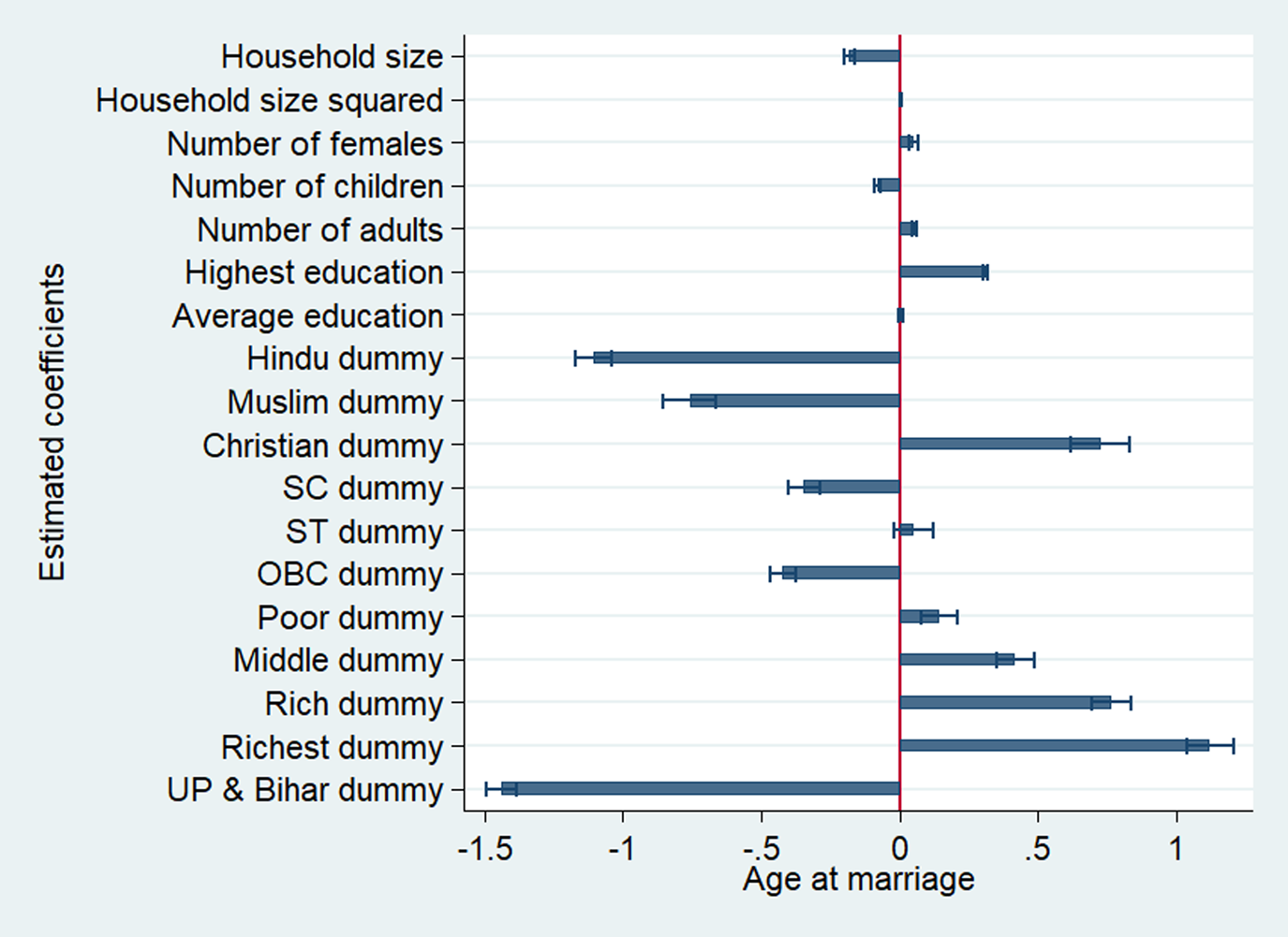
Figure 2. Estimated coefficients for age at marriage.
Table 1. Descriptive statistics
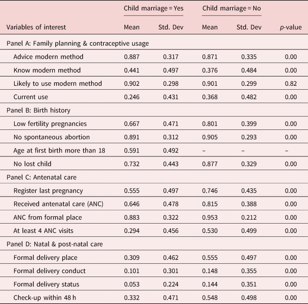
Note: The p-value reports the results from the t-test that the outcome variables for the two groups of women (those married before the age of 18 and after) are equal. Advice modern method: What method did the one who advised you to adopt family planning method advise you? 1 if female sterilization, male sterilization, IUD, daily pills, weekly pills, injectable, male or female condom, 0 if rhythm abstinence, withdrawal or other traditional methods. Know modern method: Which ways or methods have you heard about? 1 if modern and 0 if rhythm abstinence, withdrawal or other traditional methods. Likely to use modern method: Do you intend to use any modern method of family planning at any time in the future? If yes, which method would you prefer to use? 1 if modern and 0 if traditional methods. Current use: Are you/your husband currently doing something or using any method to delay or avoid getting pregnant? 1 = Yes, 0 = No. Low fertility pregnancies: Now I would like to ask you, about the number of times you were pregnant which resulted in live births, still births or abortions since January 1, 2004? 0 if greater than equal to 2, 1 if less than 2. This sample is restricted to age group of 20–24. Having 2 or more pregnancies before turning 24 is considered as an indicator for high fertility. No spontaneous abortion: Did any of your pregnancy terminate in spontaneous abortion? If yes, how many? 1 = No, 0 = Yes. Age at first birth more than 18: How old were you at the time when your first child was born? 0 if less than 18 and 1 otherwise. No lost child: A dummy constructed from the sum of number of boys died and number of girls died. 0 = child was lost, 1 = No child was lost. Register last pregnancy: Did you register your last pregnancy? 0 = No, 1 = Yes. Received ANC: When you were pregnant with (name/ the still birth), did you receive antenatal care? 1 = Yes, 0 = No. ANC from formal place: Where did you receive antenatal care for last pregnancy? 0 = Home, 1 = Government or private institutions. At least 4 ANC visits: How many times you received antenatal check-up during last pregnancy? 0 = Less than 4, 1 = More than or equal to 4. Formal delivery place: Where did your last delivery take place? 0 = Home, 1 = Government or private institutions. Formal delivery conduct: Who conducted your last delivery? 0 = traditional personnel (Dai, relatives), 1 = modern health personnel. Formal delivery status: Was the delivery normal or cesarean or assisted? 1 = Caesar or assisted, 0 = normal delivery. Check-up within 48 h: Did you have any check-up within 48 h after delivery? 1 = Yes, 0 = No. So, higher values will indicate incidence of better outcomes i.e. lower values for child marriage (which is yes) means lower incidence of better outcomes.
To control for the recall bias, we observe the health behavior and outcomes of women in the age-group of 20–24 separately, as this is the preferred age for pregnancy, especially if the women are married early.
4. Datasets used in this paper
The dataset that used in this paper is derived from the District Level Household Survey (also referred to as DLHS-3) conducted in India during 2007–08. The DLHS-3 survey covered about 720,320 households from 28 states and 6 union territories in India. From these households, 643,944 ever-married women aged between 15–49 years were interviewed to record their reproductive and birth history. The data related to contraceptive awareness and usage, birth history, antenatal, natal and post-natal care have been used from the ever-married questionnaire, while detailed information about the household and its members were derived from the household questionnaire. This dataset was eventually mapped to the detailed district level rainfall data derived from the Indian Meteorological Department, Ministry of Earth Science using the unique district identifier.
As the objective of this work is to causally estimate the impact of incidence of child marriage on different health utilization variables related to different stages of the woman's life—ranging from family planning and pregnancy to childbirth, the variable of interest in this context is whether the respondent aged 15–49 years was married before she turned 18 or after, i.e. the incidence of child marriage dummy takes a value of 1 if she was married as a child and 0 otherwise. On the other hand, sixteen different outcome variables has been considered in the analysis, which has been categorized under four broad sub-heads—attitude towards and actual usage of modern family planning methods, past and present birth history and uptake of antenatal, natal and post-natal care made available to the respondent by the government. The responses of these women to the various questions asked in the ever-married questionnaire have been used as outcome variables. All the sixteen outcome variables discussed in this section have been constructed in such a way that a higher value is indicative of a better outcome while a lower value means a worse outcome. So, the lower means associated with child marriage will mean lower incidence of the better outcomes and higher incidence of the worse outcomes. Each of the outcome variables used in the analysis has been discussed in detail in the four subsections that follow.
4.1 Family planning and contraceptive usage
The analysis begins by discussing the variables related to family planning and contraceptive usage, which have been captured using four dummy variables, namely, advice modern method, know modern method, likely to use modern method and current use. Towards this end, the responses of these women to the following questions: “Did anyone advise you/your husband to adopt any modern family planning method?”; “Which ways or methods have you heard about?”; “Do you intend to use any modern method of family planning at any time in the future? have been used. If yes, which method would you prefer to use?” and “Are you/your husband currently doing something or using any method to delay or avoid getting pregnant?” to construct the respective family planning and contraceptive usage variables. The advice modern method variable takes a value of 1 if the response to the question “Did anyone advise you/your husband to adopt any modern family planning method?” was yes to male or female sterilization, IUD, daily pills, weekly pills, injectable, male or female condom and 0 if the response was yes to rhythm abstinence or withdrawal. Similarly, the dummy know modern method is assigned a value 1 if the respondent heard about modern methods such as male or female sterilization, IUD, daily pills, weekly pills, injectable, male or female condom and 0 if she heard about rhythm abstinence or withdrawal only. The dummy likely to use modern method was created from the question “Do you intend to use any modern method of family planning at any time in the future? If yes, which method would you prefer to use?”. The variable was coded 1 and 0 just like the previous variables. Finally, for current use, a value of 1 has been assigned if the couple was found using any method to delay or avoid getting pregnant and 0 otherwise.
4.2. Birth history
In this subsection of the paper, estimating the effect of child marriage on age at first childbirth, fertility and infant mortality have been focused. These variables are of particular interest as women who marry early are expected to be under-aged at the time of first birth, i.e. their age at the time of first birth is less than 18 and have higher number of pregnancies, including complicated ones, which may put their own lives as well the lives of their unborn child at stake. For the first variable, the response of the woman to the following question: “How old were you at the time when your first child was born?” has been used. The age response has been coded in such a manner that the dummy age at first birth more than 18 years takes a value of 0 if the age is less than 18 and 1 otherwise. The social norms that dictate the marriage and family system in India, requires that early marriage is immediately followed by childbirth, thereby the onset of early motherhood for adolescent girls. The dummy variable low fertility pregnancies used next in the analysis was created from the question: “Now I would like to ask you, about the number of times you were pregnant which resulted in live births, still births or abortions since January 1, 2004?” The dummy low fertility pregnancies has been coded as 0 if the number of pregnancies were greater than equal to 2 and 1 if they were not pregnant more than once. This sample is restricted to only women belonging to the age group of 20–24 years as having 2 or more pregnancies before turning 24 has been considered an indicator for high fertility. Next, the difference between the number of livebirths and children who died is used to create the third variable of interest, No lost children, where 1 means no child was lost by the woman and 0 otherwise. Similarly, the variable No spontaneous abortion has been created from the following question “Did any of your pregnancy terminate in spontaneous abortion? If yes, how many?”. This dummy variable takes a value of 1 if the response to the question is No and 0 otherwise.
4.3. Antenatal care
In this and the next subsection, the effects on ante-natal and natal and post-natal care have been examined as it is considered to be an important determinant of maternal as well as child health, both during pregnancy and thereafter. The variables considered to capture these effects include whether the pregnant woman registered their last pregnancy, received ANC or not, ANC was received from formal place or not and if the number of ANC visits received during pregnancy is at least 4. Each of these four outcome variables were derived from the following four questions. If response to the question “Did you register your last pregnancy?” is positive, register last pregnancy is coded as 1 and 0 otherwise. The question “When you were pregnant with (NAME/ THE STILL BIRTH), did you receive antenatal care?” has been exploited and the variable, received ANC has been coded as 1 if the response is positive and 0 if not. The question “Where did you receive antenatal care for last pregnancy?” is used to code the dummy ANC from formal place as 0 if the response was home and 1 if the response was government or private institutions. The last variable used, at least 4 ANC visits capture how many times antenatal check-up was received by the woman during her last pregnancy. The variable has been coded 1 if the number of ANC visits received is four or more, and 0 if not.
4.4. Natal and post-natal care
In this final subsection, the four variables that capture the extent of healthcare facilities utilized by the pregnant woman during childbirth and thereafter have been discussed, given that the government has implemented several policies making these health facilities widely available and accessible. Particular focus is on identifying whether the place of delivery is formal or informal, who conducted the delivery, delivery status and whether check-up was received within 48 h of birth. Each of these four variables were constructed using the responses to the following four questions: “Where did your last delivery take place?”; “Who conducted your last delivery?”; “Was the delivery normal or cesarean or assisted?” and “Did you have any check-up within 48 h after delivery?”. The first variable formal delivery place was assigned a value of 0 if the delivery took place at home and 1 if at a government or private institution. The second variable formal delivery conduct, similarly, was coded in such a way that if deliver was conducted by traditional personnel like dai (midwife or wet nurse) or relatives, the variable takes a value of 0 and 1 if the delivery was performed by trained personnel. On the other hand, the dummy Delivery status takes a value of 1 if the response is cesarean or assisted and 0 if the delivery was normal. Finally, the variable Check-up within 48 h, was given a value 1 if the respondent received check-up within 48 h of delivery and 0 otherwise. Descriptive statistics for each of the outcome variables by incidence of child marriage is reported in Table 1 while Table A1 in the Appendix reports the same outcome variables by their state of residence. Table A2 in the Appendix on the other hand presents the descriptive statistics for the control variables used in this analysis.
5. Regression results
The regression results estimated using equation (1), illustrating the effect of child marriage on various health outcomes are presented in this section of the paper. The estimates from family planning and contraceptive usage and birth history regressions are reported in Tables 2, 3, while those related to antenatal, natal and postnatal care are presented in Tables 4, 5. The first column in Tables 2–5 reports the OLS results for the whole sample, while the next column reports the IV results for the same sample. The results presented in the third and fourth columns of each Table, on the other hand, report the results separately for UP & Bihar and women aged 20–24 years respectively.
Table 2. Regression estimates of family planning and contraceptive usage
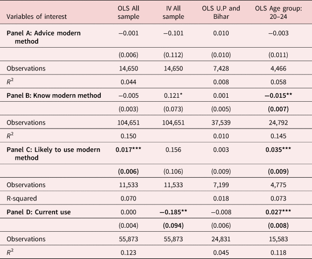
Note: The coefficient of incidence of child marriage related to the outcome variables has been reported. All regressions also control for the usual control variables such as household size, household size squared, number of females, number of children aged 5–18 years, number of adults in the household, highest education in the household, average education in the household, religion categories (Hindu, Muslim, Christian and Others), caste categories (General, SC, ST and OBC), region categories (urban or rural) and asset quintiles based on the wealth index (poorest, poor, middle, rich and richest). State-fixed effects are controlled in each regression. Standard errors are clustered at the PSU-level. Clustered standard errors are presented in parenthesis. ***p < 0.01, **p < 0.05, *p < 0.1. See footnote of Table 1 for a detailed discussion of the different variables used as the outcome variables.
Bold indicates that the regression coefficients are statistically significant.
Table 3. Regression estimates of birth history
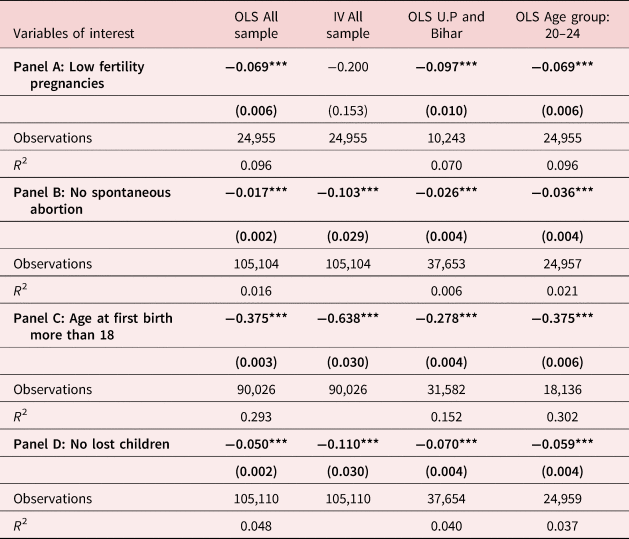
Note: See footnote of Table 2 for the control variables used in the analysis and footnote of Table 1 for a detailed discussion of the different variables used as the outcome variables. The coefficient of incidence of child marriage related to the outcome variables has been reported. State-fixed effects are controlled in each regression. Standard errors are clustered at the PSU-level. Clustered standard errors are presented in parenthesis. ***p < 0.01, **p < 0.05, *p < 0.1.
Bold indicates that the regression coefficients are statistically significant.
Table 4. Regression estimates of antenatal care
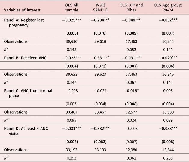
Note: See footnote of Table 2 for the control variables used in the analysis and footnote of Table 1 for a detailed discussion of the different variables used as the outcome variables. The coefficient of incidence of child marriage related to the outcome variables has been reported. State-fixed effects are controlled in each regression. Standard errors are clustered at the PSU-level. Clustered standard errors are presented in parenthesis. ***p < 0.01, **p < 0.05, *p < 0.1.
Bold indicates that the regression coefficients are statistically significant.
Table 5. Regression estimates of natal and postnatal care
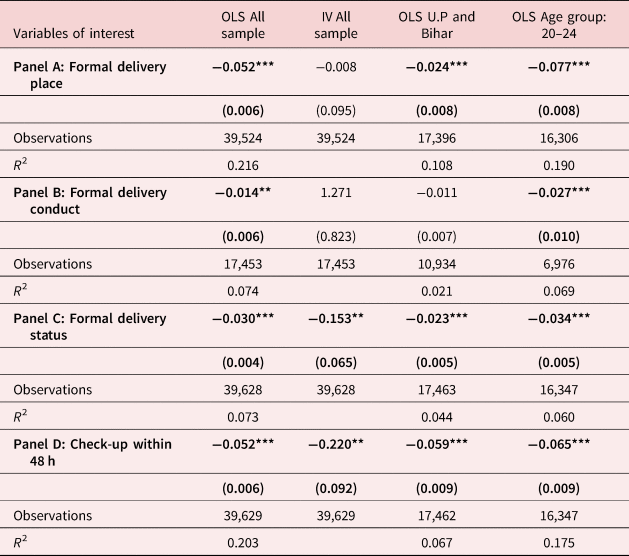
Note: See footnote of Table 2 for the control variables used in the analysis and footnote of Table 1 for a detailed discussion of the different variables used as the outcome variables. The coefficient of incidence of child marriage related to the outcome variables has been reported. State-fixed effects are controlled in each regression. Standard errors are clustered at the PSU-level. Clustered standard errors are presented in parenthesis. ***p < 0.01, **p < 0.05, *p < 0.1.
Bold indicates that the regression coefficients are statistically significant.
The results with family planning and contraceptive usage as the dependent variables and incidence of child marriage as the variable of interest are presented in Table 2. The regression results related to advice received regarding modern family planning methods is presented in panel A of Table 2, followed by results related to knowledge about modern methods, likelihood to use modern methods and current contraceptive use in the panels B-D of Table 2 respectively. The coefficients related to only incidence of child marriage have been reported from each regression, while the regression results with full set of controls is presented in Table A3 in the Appendix.
The OLS results presented in the first column of Table 2 suggest that incidence of child marriage is negatively related to receiving advice regarding modern family methods, knowledge regarding modern family methods, though the effects are not statistically significant. Though likely to use modern methods bears a positive association, current usage has no significant association with child marriage. The IV results in column (2), however, demonstrate that current usage is negatively associated with incidence of child marriage and is this association is statistically significant—women who are married before reaching her 18th birthday are 18.5pp less likely to currently use these modern methods. The coefficients associated with the other outcomes are insignificant or is weakly significant. Given the endogeneity problem associated with the OLS estimates, more weight is put on the IV estimates, which are the preferred results. The first stage results from the IV regressions are discussed later.
However, given that the instrument is average rainfall at the district level, there is not enough variation in rainfall across different districts in UP & Bihar. Therefore, only the OLS results for UP & Bihar and women aged 20–24 years have been presented, which can be directly compared to the OLS estimates for the whole sample in the first column of Tables 2–5. From the results in the third column in Table 2, it can be seen that for U.P & Bihar, the coefficients are insignificant. Interestingly, the results in column (4) confirm the hypothesis that younger women (20–24 years) are more vulnerable and are less likely to know about modern contraception methods, however they are more likely to use contraception. Usage of modern contraception methods is also more among them. The overall results presented in Table 2 therefore suggest that the effect of incidence of child marriage varies across both states and different age group of women.
The estimates in Table 3 report the regression coefficients that illustrate the effect of child marriage on birth history of the respondent, captured via questions related to maternal age at first birth, number of pregnancies for women in the 20–24 age cohort (used as an indicator for high fertility), incidence of spontaneous abortion and infant mortality. The OLS and IV results presented in columns (1) and (2) of panel A in Table 3 report that the probability of high fertility pregnancies defined by having 2 or more pregnancies increases by 6.9pp (significant) and 20.0pp (insignificant) respectively for women who marry early. From Panel C in Table 3, it is found that women who get married before reaching her 18th birthday are 37.5pp and 63.8pp more likely to have their first birth before they attain the age of 18. Similarly, the OLS results presented in columns (3) and (4) show that women married before reaching their 18th birthday in Bihar and U.P as well those in the 20–24 age group are significantly affected across all outcome variables and the results for UP & Bihar and 20–24 age group are either similar or slightly higher compared to the overall sample estimates. These women are also more likely to have spontaneous abortion or miscarriages and lose a child after they are born.
The regression coefficients of Table 4 report the results related to antenatal care, received by women during pregnancy. Robust evidence that incidence of child marriage is significantly related to utilization of antenatal care has been found. Based on the OLS estimates, women who get married before they attain the age of 18 are 2.5pp, 2.3pp and 3.1pp less likely to have registered their last pregnancy, received antenatal care (ANC) and made at least four ANC visits. The IV estimates, however, are significantly higher compared to the OLS estimates for the whole sample. Women who marry early are 20.4pp, 33.1pp and 33.2pp less likely to receive the same antenatal care services respectively. The results presented in column (3) demonstrate that the probability of not registering their last pregnancy is significantly more in Bihar and U.P compared to the overall sample. Women who are married before reaching 18 years in these states are 4.8pp more likely not to resister their last pregnancy compared to 2.5pp for the whole sample and 3.2pp for women in the 20–24 age group (column 4). The probability of not receiving ANC, on the other hand, is 2.3pp, 3.1pp and 2.9pp more among those married as a child in the overall sample, UP & Bihar and for the 20–24 age group i.e. women residing in UP & Bihar is worse affected in terms of being deprived of the necessary ANC visits. While the estimated results are insignificant for the states of UP & Bihar for the variable—At least 4 ANC visits; the estimated coefficients are significantly lower for those women belonging to the 20–24 age group.
Finally, Table 5 reports the results related to natal and post-natal care received by women during delivery. Robust evidence that incidence of child marriage is significantly related to utilization of healthcare facilities has been found, captured via delivery at a formal place such as a government or private institution or at home; conducted by formal or traditional personnel; whether delivery was normal or cesarean and whether check-up was received within 48 h of delivery or not. Based on the OLS estimates, evidence that women who get married before reaching her 18th birthday are 5.2pp, 1.4pp, 3.0pp and 5.2pp less likely to receive formal delivery facilities such as delivering at a government or private institution, by modern health personnel, via cesarean section and to receive check-up within 48 h within delivery, have been found respectively. The IV estimates, as expected are significantly higher to the tune of 15.3pp and 22.0pp for formal delivery place and check-up received within 48 h of delivery respectively. The IV regression results, however, related to formal delivery place and formal delivery conduct is not statistically significant. While the regression coefficients related to UP & Bihar are either similar or significantly lower compared to the results for overall sample presented in column (1), the estimated negative effects are significantly higher among women aged 20–24 years. The actual impact of child marriage on these sub-groups of women, however, may be larger in magnitude. The overall results of the paper presented in Tables 2–5 therefore suggest that child marriage has detrimental health effects, possibly as the first autonomy effect may outweigh the resource effect. Young women who are married off early are found to be particularly at risk and this only confirms the suspicion that autonomy of women has an important role to play in this context.
The relatively larger magnitude of the IV estimates suggests that the OLS results might be affected by measurement error. The outcome variables such as age at first birth, if received ANC, if made at least 4 ANC visits might be prone to recall bias as mothers often cannot accurately recall details of their pregnancy, experiences during childbirth and birth history [Fagbamigbe and Idemudia (Reference Fagbamigbe and Idemudia2015), Dutamo et al. (Reference Dutamo, Assefa and Egata2015), Godha et al. (Reference Godha, Gage, Hotchkiss and Cappa2016), Tripathi and Singh (Reference Tripathi and Singh2017), Gopalan et al. (Reference Gopalan, Silverwood, Salman and Howard2019)]. The recall biases arise due to retrospective nature of the data. Women with more education may have better recalled their birth history, the caring they received during antenatal, prenatal and neonatal periods compared to those who are less educated. Similar variation in recall may arise depending on their number of engagements in their day to day life, their level of stress or extent of domestic violence. Also, mothers who had recently given their last birth might recall the care they received in the immediate past compared to those had their last birth prior to them [Asamoah and Agardh (Reference Asamoah and Agardh2017), Rurangirwa et al. (Reference Rurangirwa, Mogren, Ntaganira and Krantz2017)].
Another reason for which the IV estimate might be larger than the OLS estimate is that while OLS estimates capture the average difference in outcome variables for those who are married prior to attaining 18 years of age vs those who are married after attaining 18 years; the IV estimate is capturing the effect of marrying prior to attaining 18 years only for those women whose who were married at an early age due to household poverty caused due to lack of adequate rainfall in those districts. This is known as the “local average treatment effect” (LATE). However, there are some girls who would any way be married only after attaining 18 years or later as the households in which they belong might be aware of the adverse consequences of child marriage a-priori. On the other hand, there are girls who would have married before reaching 18 years even if the average rainfall and hence agricultural yield in the districts they reside are high. Hence the IV estimate gives us the effect of child marriage on only the compliers – the set of girls who were married prior to attaining 18 years of age due to household poverty arising out of low average annual rainfall.
We report the first stage regression results for our IV estimates in Table 6. Each of our outcome variable regarding family planning and contraceptive usage, birth history, antenatal care, natal and post-natal care is negatively correlated with average annual rainfall in the districts. These results are significant even at 1%. The F-statistics for the first stage regressions reported in Table 6 show that average annual rainfall is a strong instrument for child marriage. With the exception of incidence of formal delivery conduct, we find that the F-statistics for the first stage regressions for all the other outcome variables is consistently greater than 10.
Table 6. First-stage results
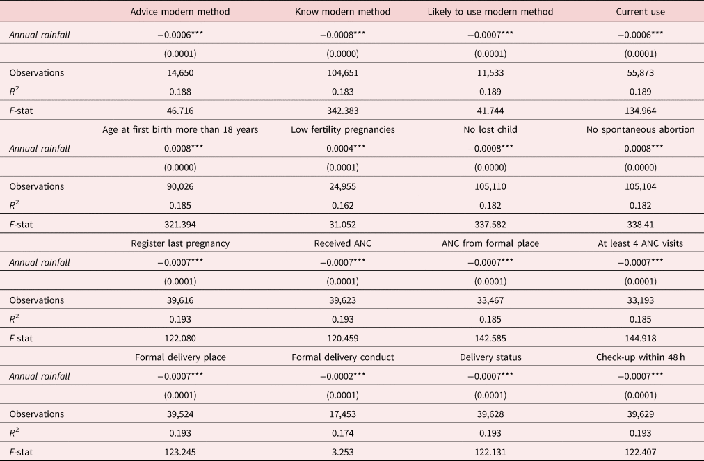
Note: State-fixed effects are controlled in each regression. Standard errors are clustered at the PSU-level. Clustered standard errors are presented in parenthesis. ***p < 0.01, **p < 0.05, *p < 0.1. The coefficients related to only the IV, Annual rainfall, is the average annual rainfall in the district during 2005 and 2006. These are the coefficients associated with the Annual rainfall from the first stage of the respective IV regressions, with the outcomes of child marriage as the dependent variable and Annual rainfall as the variable of interest. See footnote of Table 3 for the control variables used in the analysis and footnote of Table 1 for a detailed discussion of the different variables used as the outcome variables.
The Indian economy is highly dependent on agriculture and agriculture allied activities, which depends to a large extend on the average rainfall. Geographically, the districts with higher average rainfall prosper better than others, especially if they are solely dependent on farm productivity. The age at marriage depends on the prosperity of the households, more so, if they reside in rural areas where the economy is majorly linked to farm productivity either directly or indirectly. Child marriages are more common in the districts in which the average rainfall is lower than others. The households are unable to feed the girl children for long and hence sell them off in the form of marriage as the dowry required to get the younger girls married is substantially lower. This leads to a positive association between the average annual rainfall and the average age at marriage as can be seen from the scatter plot in Figure 3.
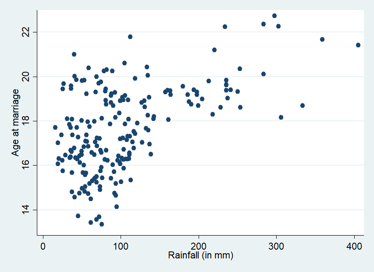
Figure 3. Association between district wise annual rainfall and average age at marriage.
Rainfall is directly and positively related to agricultural productivity in India. Districts that receive higher annual rainfall have greater agricultural and agricultural-allied production. Average wealth of households residing in districts with higher average annual rainfall is hence, more than those in other districts. We present a graphical representation of the correlation between district wise average annual rainfall and average household wealth in Figure 4.
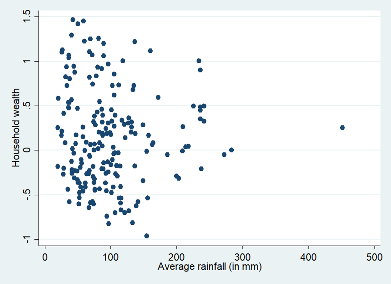
Figure 4. Association between district wise annual rainfall and average household wealth.
Rural households in India are solely dependent on the produce from agriculture and allied sectors that are directly and heavily dependent on the average rainfall in the district. In the supplementary material, we have included a scatter plot (Extra Figure 1, which would be made available upon request) showing the association between district wise average annual rainfall and average household wealth only for those rural households possessing agricultural land. The nature of association is almost similar to that the association when we restrict the sample only to the rural households (Figure 4). The landless households residing in rural regions are similarly deprived of their manual labor income if the farm production is less due to lesser rainfall. Hence, we restrict our sample only to the rural regions irrespective of if they own agricultural land. This also provides us a larger sample sizeFootnote 2.
One might be interested to see if the IV first stage would produce null effect of average rainfall on age at marriage, for the urban households, since we have restricted our sample to the rural households. We present these results in Appendix Table A4. We find that the magnitude of the association between the outcome variables and average rainfall in the urban localities are 1.5 to 3.5 times lower (apart from the incidences of formal delivery conduct) compared to those in the rural localities (see Table 6). The results are significant however, since a sizeable part of even the urban households in India is linked to agriculture-allied activities such as food processing, marketing and distribution of the agricultural products. The F-statistics in case of incidences of receiving advice about modern contraceptives, likely to use modern contraceptive, low fertility pregnancies and incidences of formal delivery conduct suggests that average annual rainfall is a weak instrument for such outcomes in the urban locality.
To test the probability of rejecting at least one true null hypothesis in the family of 16 hypothesis that we consider, we have used the Romano Wolf Multiple Hypothesis correction methodology. It uses resampling methods like bootstrapping to control for the familywise error correction asymptotically. This method has greater capability of correctly rejecting false null hypothesis and is hence, considered superior to earlier multiple hypothesis correction tests [for detailed discussion, see Clarke et al. (Reference Clarke, Romano and Wolf2020)]. We find that the probability of rejecting true null hypothesis regarding the effect of child marriage on birth history, utilization of antenatal care services, natal and postnatal care services is less than 1% for the OLS regressions. The effect on the awareness regarding family planning methods and contraceptive usage are insignificant. The results are similar for the IV regressions except for the incidences of ANC received from formal place which is insignificant, and incidences of formal delivery conduct which is significant at 5%. The Romano Wolf Multiple Hypothesis results for the OLS and IV regressions are reported in Panels A and B in Table 7 respectively.
Table 7. Romano–Wolf test
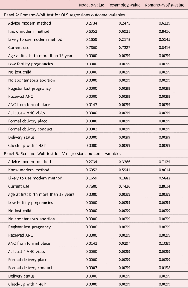
Note: The resample p-values in column 2 are obtained after 100 bootstraps.
Another concern in estimating the impact of child marriage is that incidence of child marriage might be subject to measurement error. One of the assumptions of classical measurement error is that the error in the proxy variable of interest (child marriage in this context) must be statistically independent of the proxy variable of interest. Age at marriage is often prone to measurement error [for detailed discussion, see Mensch et al. (Reference Mensch, Singh and Casterline2005)]. Misreporting of age at marriage defies this assumption as age is often rounded off to the closest age in whole number, which is prone to be arbitrary and subject to biases. Those who had married close to attaining 18 years tend to report it as 18 or higher, being aware about the legal age at marriage in India (which is 18 years). This is a classic example of social desirability bias. Also, it might involve recall bias as the age at marriage is self-reported and hence is affected by their level of education and memory. This violates the assumption of classical measurement error as the measurement error, that is, the difference between the original age at marriage and the reported age at marriage, is not statistically independent of the (probable) misreported age of marriage. Since our variable of interest is a dummy variable representing if she was married prior to attaining 18 years, a non-classical measurement would render the IV estimates inconsistent. The bias in IV estimates would depend on the misclassification rates in the child marriage variable. Greater misclassification in the instrument leads to smaller first stage coefficient making the IV estimate biased upward (in magnitude). To address this problem, we introduce a robustness check whereby we replace the child marriage indicator by another alternative indicator of early marriage, that is, if the girl was married prior to attaining 17 years of age. Our results are largely similar to those reported in columns (1)–(2) of Tables 2–5 with the exception that the negative OLS estimates for advice modern method and know modern method is now significant; and the negative OLS estimate for formal delivery conduct is now insignificant and the positive IV estimate for the same is now significant. The results for these are reported in Appendix Table A5.
From Table 8, where the results related to the falsification test have been presented, estimated by replacing the dependent variable with the chances of having twins and being currently married (one at a time) suggest that the results are non-spurious and provide validity to the results estimated using equation (1) and presented in Tables 2–5 to be causal in nature.
Table 8. Falsification test

Note: The Twin dummy variable takes a value of 1 for their occurrences and 0 otherwise. Not currently married dummy is a dummy variable that takes the value of 1 for separated/deserted/divorced/widowed and 0 for being currently married. See footnote of Table 2 for the control variables used in the analysis. State-fixed effects are controlled in each regression. Standard errors are clustered at the PSU-level.
6. Conclusion
Despite the introduction of strict marriage laws in India that consider marriage of adolescent girls under the age of 18 as illegal and initiation of several national and state sponsored conditional cash transfer programs with the intention of providing incentives to parents to voluntarily delay the marriage of their daughters, India still remains home to the world's largest number of child brides. Previous research provides evidence that early marriage of women not only limits the educational attainment, employment opportunities and overall human capital acquisition of the women themselves but also has intergenerational effect on the health and education outcomes of their children. However, the literature fails to provide a complete understanding of the causal impact of child marriage on reproductive and pregnancy related choices of women, using rigorous empirical methodology that control for the endogeneity problem inherent in the decision of the household to get their daughters married early, eliminate recall bias and also capture the variation in these effects across different states of residence and age groups.
In the current paper, strong evidence that early marriage of women results in reduced likelihood of using modern family planning methods such as male or female sterilization, daily or weekly birth control pills and condoms has been found. Those in the younger age-group of 20–24 are less likely to have heard about these modern methods due to their limited education and exposure. Child marriage also significantly increases the probability of having spontaneous abortion or miscarriage, likelihood of the first child being born before attaining the legal age of marriage, having two or more pregnancies early in life and reduces the chances of survival of the child born. In addition, they are also less likely to register their last pregnancy, receive antenatal care and make at least four antenatal visits which is considered as bare minimum. The regression results from the IV regressions, in addition to confirming that a causal effect is indeed there also indicates that the significant negative impact of child marriage may be far worse than suggested by the OLS estimates.
When the states of Uttar Pradesh and Bihar have been particularly focused, it is found that women who marry early in these states are significantly less likely, register their last pregnancy and more likely to have higher fertility and lose a child compared to their counterparts residing in the other states. Finally, particular focus is done on the 20–24 age cohort in order to minimize the recall bias and get a better understanding of the current uptake of publicly funded healthcare facilities, being made available and easily accessible by the government, it is found that almost all the estimated coefficients are significantly negative and sometimes slightly higher in magnitude than that of the whole sample. The results related to women belonging to the 20–24 age group therefore suggest that while they are more likely to currently use modern methods of contraception compared to the overall sample, they are particularly less likely to use formal healthcare facilities during delivery possibly due to the presence of social and cultural barriers that they unable to break due to the lack of autonomy or voice in the household decision making.
Supplementary material
The supplementary material for this article can be found at https://doi.org/10.1017/dem.2022.29.

