


1. Introduction
Instrumental variables (IV) estimation has been widely used in empirical social science to estimate causal effects in the presence of self-selection (Sovey and Green, Reference Sovey and Green2011; Aronow and Carnegie, Reference Aronow and Carnegie2013; Blackwell, Reference Blackwell2017). Self-selection may be driven by the same beliefs and incentives that are of central interest to our theories, as people anticipate the effect of treatment. However, IV estimands only identify the Local Average Treatment Effect (LATE) for compliers: the subpopulation responsive to the instrument(s) (Imbens and Angrist, Reference Imbens and Angrist1994). To understand self-selection incentives and the consequences of messaging among particularly enthusiastic consumers, we must extrapolate to the other two unobserved principal strata, especially those who would be exposed to the treatment even without the observed instrument (Heckman and Urzua, Reference Heckman and Urzua2010).
Estimation strategies that address non-compliance are particularly valuable when subjects can only be encouraged or incentivized, rather than required, to participate in a treatment. For instance, when autocratic governments use propaganda to persuade people of their performance, or candidates for office attempt to distinguish themselves by their policy proposals, we rarely can completely control access to the political messaging. Instead, individuals must decide whether to consume the political message based on some smaller incentive or cost. However, those smaller incentives or costs can only be expected to shift a subset of respondents. Those that fail to respond to weak encouragements may of the most interest to social scientists: how does the treatment affect those that are willing to undergo costs to acquire it? Given widespread evidence of heterogeneity in how people respond to persuasive messaging, limiting analysis to encouragements alone gives a narrow window into the overall consequences of political messaging (DellaVigna and Gentzkow, Reference DellaVigna and Gentzkow2010; Peisakhin and Rozenas, Reference Peisakhin and Rozenas2018; Jun and Lee, Reference Jun and Lee2019).
These issues arise in the study of the effects of foreign media that rely on variation in the costs of access. When these costs are insufficient to completely shut off the foreign media some fraction of the population may be “always-takers.” The behavior of this group can be of central to understanding the effect of media openness on political authority (Gentzkow and Shapiro, Reference Gentzkow and Shapiro2006). Suppose that those opposed to the government are also enthusiastic consumers of foreign media. If such individuals seek out foreign media to placate themselves, then they might oppose the regime more if foreign media were more thoroughly blocked (Peisakhin and Rozenas, Reference Peisakhin and Rozenas2018). This concentrated increase in opposition can be more dangerous than even broader sorts of opposition. If, however, people seek out information that confirms their beliefs, we might find that foreign media reinforces the beliefs of those most opposed to the regime.
In this paper, we offer an approach to extrapolate IV estimates to the average treatment effects of always-takers and never-takers. While it is impossible to avoid assumptions in this extrapolation, we demonstrate the benefits of adopting the approach to explicitly model selection based on an underlying utility framework developed in Heckman and Vytlacil (Reference Heckman and Vytlacil2005). In this approach individuals choose to comply or not based on unobserved latent utility. Specifically, we apply the marginal treatment effect (MTE) approach developed in the latent index selection literature whose assumptions can be shown to be equivalent to the IV model described by Imbens and Angrist (Reference Imbens and Angrist1994) (IA IV model), written in terms of an underlying choice model (Vytlacil, Reference Vytlacil2002).
Our target of interest is the MTE, the average treatment effect for the individual whose utility calculations places her at the margin of selecting into treatment. This quantity characterizes individual level heterogeneity in terms of latent utility for the treatment.Footnote 1 By using this framework, we are given a substantive interpretation of the instrument, that it shifts an individual's incentive to take up treatment. We use this variation to answer questions about models of political persuasion.
Given this framework, we characterize the assumptions necessary to extrapolate IV estimates to always-takers and never-takers. Following (Brinch et al., Reference Brinch, Mogstad and Wiswall2017), we characterize two parametric assumptions that are sufficient for point identification. These are, first, separability of the outcome processes, second, the linearity of the average outcomes for both treatment and control in terms of the unobserved latent utility. Together, these assumptions guarantee point identification of the ATE of always-takers and never-takers for binary instruments. However, for many social scientific applications, these parametric assumptions are implausible. For these cases, we show that it is still possible to achieve partial identification, setting bounds that depend on the stringency of assumptions.
Specifically, we apply the strategy of Mogstad et al. (Reference Mogstad, Santos and Torgovitsky2018) to construct sharp bounds for the ATEs of always-takers and never-takers. It turns out that many observable treatment effect parameters (e.g., the IV estimand, the OLS estimand) can be written as weighted averages of MTE functions, where the weights are identifiable from data. Those observable treatment effect parameters provide restrictions on the unknown MTE function, hence on the possible values (i.e., bounds) of ATEs of always-takers and never-takers. In other words, the identifiable treatment effect parameters act as constraints in a linear program by limiting the possible parameter space of the MTE function. This information can be flexibly combined with substantively motivated structural assumptions, for instance, assuming that the MTE is monotonically decreasing, where those who are reluctant to take up treatment are those who are least likely to benefit.Footnote 2
When implementing the linear program, researchers need to specify the basis functions of the MTE function. We offer two approaches. First, researchers can use constant splines. Such an approach is fully non-parametric and, when an IV has discrete support, it computes the sharp bound of the target parameter (Mogstad et al., Reference Mogstad, Santos and Torgovitsky2018). The fact that this approach is fully non-parametric suggests that the assumptions made in the typical IA IV model are already sufficient for identification.
However, identification does not guarantee informative estimates. The MTE framework allows researchers to introduce additional assumptions for extrapolation. For instance, if an instrument decreases the cost of treatment, it may be possible to make specific assumptions about the elasticity of those costs. In the absence of such a theory, we can proceed by re-estimating under varying assumptions. In addition, we show that the linear programing approach, based on Mogstad et al. (Reference Mogstad, Santos and Torgovitsky2018) and Mogstad and Torgovitsky (Reference Mogstad and Torgovitsky2018) performs better than other partial identification approaches.Footnote 3
Finally, in the latter part of the paper, we replicate the Kern and Hainmueller (Reference Kern and Hainmueller2009) study of the effects of exposure to West German television on pro-communist sentiment among people in the German Democratic Republic. To address the endogeneity of media exposure, Kern and Hainmueller (Reference Kern and Hainmueller2009) use geographically determined variation in the accessibility of Western television signals as an instrument for exposure. We extrapolate to set bounds on the causal effect among those whose consumption of Western media was not deterred by a weak television signal (always-takers) and for those who would not be exposed even if the signal were strong (never-takers). The extrapolated results from the linear program are especially informative for always takers: there is a negative effect of watching West German TV on their support of communism. Given this population is particularly opposed to communism overall, we would expect the counterfactual where West German TV were completely closed off for East Germany to mollify these strong opponents of the regime. These results are consistent with the findings in Peisakhin and Rozenas (Reference Peisakhin and Rozenas2018). In that context, among “pro-Russian” Ukrainians, the effect of Russian television is positive, while among those who have lower pro-Russia support, the effect of Russian television is negative.
This paper relates to three lines of methodological literature. First, it complements existing strategies for extrapolating LATE (Heckman and Vytlacil, Reference Heckman and Vytlacil2005; Aronow and Carnegie, Reference Aronow and Carnegie2013; Angrist and Fernandez–Val, Reference Angrist and Fernandez–Val2013; Bisbee et al., Reference Bisbee, Dehejia, Pop-Eleches and Samii2017), demonstrating the use of the MTE framework for political questions. Second, this paper shows how this extrapolation can help assess the external validity of experimental work in the presence of non-compliance (Hotz et al., Reference Hotz, Imbens and Mortimer2005; Hartman et al., Reference Hartman, Grieve, Ramsahai and Sekhon2015; Andrews and Oster, Reference Andrews and Oster2019). Third, our approach of reformulating the extrapolation of ATEs of always-takers and never-takers into a linear programing problem shows how a combination of optimization theory and causal inference can contribute to political methodology (Imai and Yamamoto, Reference Imai and Yamamoto2010; Abadie et al., Reference Abadie, Diamond and Hainmueller2010, Reference Abadie, Diamond and Hainmueller2015; Diamond and Sekhon, Reference Diamond and Sekhon2013).
2. Notation and assumptions
In the following we adopt a choice theoretic selection model relating an encouragement Z to the decision to opt into a treatment D. By rewriting the assumptions of IV estimation in choice theoretic terms, we obtain a clear and flexible framework for studying heterogeneity in the causal effect of D on Y. To begin, we briefly re-introduce the inference problem posed by noncompliance, focusing on the Imbens and Angrist (Reference Imbens and Angrist1994) monotonicity condition. We then present the equivalence results developed by Vytlacil (Reference Vytlacil2002) that recast these assumptions in terms of a selection equation and restate the problem in terms of marginal treatment effects.
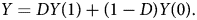
Consider the canonical causal inference problem with a binary treatment D ∈ {0, 1} and some scalar, real-valued outcome Y. Potential outcomes are Y(1) if the treatment switches on and Y(0) if the treatment switches off. The relationship between observed and potential outcomes is given by:
In addition, we can make the following assumptions on potential outcomes:
Assumption 1: Potential outcomes can be specified as: Y(d) = μ d(X) + U d, where d ∈ {0, 1}, μ 0 and μ 1 are unspecified functions of random vectors of covariates (X). U 0 and U 1 are random variables normalized so that ${\mathbb E}[ U_{0} \vert X = x] = {\mathbb E}[ U_{1} \vert X = x] = 0$ . We further assume that ${\mathbb E}[ U_{0}^{2} \vert X = x]$
 and ${\mathbb E}[ U_{1}^{2} \vert X = x]$
 exist for all x in the support of X.
Remark 1: Assumption 1 states that we can decompose potential outcomes into an additively separable function of unobservables, U d, and observables, X.
The potential outcomes framework defines a causal effect in terms of the difference between Y(0) and Y(1), an unobservable quantity. Typically, researchers take averages across individuals and estimate ${\mathbb E}[ Y \vert D = 0] -{\mathbb E}[ Y \vert D = 1]$ . The challenge for inference is that D is not independent of (Y(0), Y(1)) in observational social scientific contexts. As a result, simply differencing ${\mathbb E}[ Y \vert D = 0]$
 and ${\mathbb E}[ Y \vert D = 1]$
 can fail to produce an unbiased estimate of the average treatment effect.
Instrumental variables (IV) analysis uses variation from an instrument Z to shift the potentially endogenous treatment choice D. If Z is correlated with D, exogenous, and satisfies the exclusion restriction, the resulting variation in Y identifies the causal effect of D on Y (Mogstad and Torgovitsky, Reference Mogstad and Torgovitsky2018). Z and D can be incorporated into the potential outcomes notation, where Y(z, d) is the response for an individual given the instrument takes the value z and treatment takes the value d.
These definitions are used in the four assumptions of the standard IV estimation strategy (Imbens and Angrist, Reference Imbens and Angrist1994).
Assumption 2: Assume the following conditions hold:
1. (Independence) (Y(0), Y(1), D(z))⫫ Z;
2. (Exclusion restriction) Y(d, 0) = Y(d, 1) ≡ Y(d) with d ∈ {0, 1}.
3. (First-stage relevance) ${\mathbb E}[ D( 1) - D( 0) ] \neq 0$
 ;
;4. (Monotonicity) D(1) − D(0) ≥ 0 almost surely, or vice versa.

This framework is widely used, but this notation makes it difficult to connect the above assumptions of the IV model to theoretical models of social scientific behavior, and, for our purposes, the sort of structural assumptions needed for extrapolation. Consider, the Monotonicity condition of the IV model in Imbens and Angrist (Reference Imbens and Angrist1994), also known as the ‘no defier’ assumption. The Monotonicity condition requires all individuals to respond to the instrument the same way. This is a strong behavioral assumption: across any two different values of the instrument, it either incentivizes or disincentivizes all individuals to take up the treatment (Heckman et al., Reference Heckman, Urzua and Vytlacil2006).Footnote 4
Vytlacil (Reference Vytlacil2002) shows that these incentives can be rewritten as a natural restriction on the underlying utilities of individuals. In particular, given the exogeneity of Z, the monotonicity condition in assumption 2 is equivalent to the existence of a weakly separable selection equation:
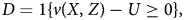
where v is an unknown function, and U is a continuously distributed random variable, what we will term latent utility.Footnote 5 The higher is latent utility, the more difficult it is to encourage uptake of the treatment. This model has its roots in an extension of Ricardo's theory of comparative advantage to occupation decisions, where individuals choose their careers on the basis of their personal productivity (Roy, Reference Roy1951).
In this model never-takers are those with such a high level of latent utility that the instrument is unable to encourage uptake of treatment, always-takers have a low latent utility, so that even when the instrument induces a low value of v(X, Z), they will opt into the treatment.
Throughout the remainder of the paper, we maintain the following three assumptions:
Assumption 3: D is determined by Equation (2).
Assumption 4: (Y(0), Y(1), U) ⫫ Z|X holds, where ⫫ denotes conditional independence.
Remark 2: Assumption 4 states that the instrument Z is exogenous with respect to both selection into treatment and outcomes after conditioning on covariates, X. Vytlacil (Reference Vytlacil2002) shows that assumption 4 implies (Y(0), Y(1), D(z)) ⫫ Z|X. In addition, if researchers are interested in estimating differences in means, assumption 4 can be relaxed to mean independence: ${\mathbb E}[ y( t) \vert Z = z,\; \, X = x] = {\mathbb E}[ y( t) \vert Z = z',\; \, X = x]$ , where z ≠ z′. Together, assumption 3 and 4 map onto the exclusion restriction. This is because Z affects D but Z is independent of potential outcomes, Y(0) and Y(1).
Assumption 5: U is continuously distributed, conditional on X.
The continuity of the distribution of the latent utility implies that we can normalize the distribution of U|X = x, Z = z to be uniform over [0, 1] for every x and z. A consequence of this normalization is that v(x, z) is a propensity score (Zhou and Xie, Reference Zhou and Xie2019),

Therefore, after renormalization, we can rewrite Equation (2) as
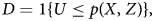
where U|X = x, Z = z ~ U[0, 1] for all z, x. Vytlacil (Reference Vytlacil2002) shows the three assumptions introduced above, along with Equation (4), are equivalent to the IV model introduced in Imbens and Angrist (Reference Imbens and Angrist1994), now in terms of a choice theoretic framework.Footnote 6
Finally, we define three functions that are essential in this paper, the marginal treatment effect (MTE) and the marginal treatment response (MTR) for Y(0) and Y(1). These are called marginal because they describe effects and responses for the hypothetically indifferent individual. Formally, the marginal treatment effect is defined as:

In words, MTE(u, x) is the average treatment effect for individuals with unobservable propensity to select into treatment, U = u and observable characteristics X = x. By conditioning the difference in potential outcomes on U = u, we can focus on the individuals whose choices are at the margin.
The MTE can be rewritten as the difference between two MTR functions, defined as:

where d ∈ {0, 1}. Each pair m ≡ (m 0, m 1) of MTR functions generates an associated MTE function: MTE(u, x) = m 1(u, x) − m 0(u, x).
3. Identifying the ATEs of always-takers and never-takers in the MTE framework
3.1 What we know and what we want to know
While we are interested in the average treatment effects of always-takers and never-takers, these quantities are not directly observed and require extrapolation. In order to identify these ATEs, we need to know the following four quantities in Table 1:
Table 1. Quantities in the ATEs of always-takers and Never-takers
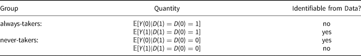
Under the assumptions described in the previous section, two of these four quantities are identifiable from the data. That is, the potential outcome of Y(1) is point identified for always-takers and the potential outcome of Y(0) is point identified for never-takers. We state the result in lemma 1.
Lemma 1: ${\mathbb E}[ Y( 1) \vert D( 1) = D( 0) = 1]$ and ${\mathbb E}[ Y( 0) \vert D( 1) = D( 0) = 0]$
 are identifiable.
Proof. See Appendix C.1. □
Given these results, we can show that the ATEs of always-takers and never-takers are weighted averages of the MTE functions and that the weights are identifiable from the data. This result is a special case of the more general results developed in Heckman and Vytlacil (Reference Heckman and Vytlacil2005) which asserted but did not formally demonstrate the following theorem.
Theorem 1: The ATE of always-takers is:

The ATE of never-takers is:

Proof. We first prove the case for always-takers:
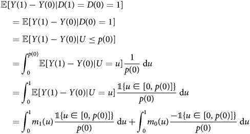
where the first equality uses the IV monotonicity assumption; the second equality uses the selection equation; the third equality uses the fact that U|U ≤ p(0) ~ unif[0, p(0)]. The case for never-takers can be proved analogously. □
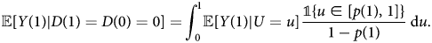
Corollary 1: From the derivation in theorem 1, for always-takers, we have:
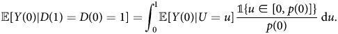
Similarly, for never-takers, we have:
Remark 4: Theorem 1 demonstrates that the ATE of always-takers is a weighted average of the MTE, where the weights are straightforward ratios of the propensity scores p(0) and p(1). This result, along with lemma 1, shows that if we can point identify ${\mathbb E}[ Y( 0) \vert U = u]$ and ${\mathbb E}[ Y( 1) \vert U = u]$
 , ${\mathbb E}[ Y( 0) \vert D( 1) = D( 0) = 1]$
 and ${\mathbb E}[ Y( 1) \vert D( 1) = D( 0) = 0]$
 are point identified, therefore, the ATEs of always-takers and never-takers would also be point identified.
The following two sections develop strategies for extrapolation of ATEs of always-takers and never-takers. The first, is a point identification result, but requires strong behavioral assumptions. The second is a partial identification result, which allows for more flexibility in modeling strategies. Our empirical analysis demonstrates each method.
3.2 Point identification of ATEs of always-takers and never-takers
Under strong assumptions, the MTE framework developed by Brinch et al. (Reference Brinch, Mogstad and Wiswall2017) can guarantee point identification of ATEs of always-takers and never-takers. Recall Remark 4, the task of point identification requires calculating two marginal treatment response pairs, i.e., ${\mathbb E}[ Y( 1) \vert U = u]$ and ${\mathbb E}[ Y( 0) \vert U = u]$
 . Further assumptions are unnecessary if P(Z) has continuous support from zero to one (Heckman and Vytlacil, Reference Heckman and Vytlacil1999, Reference Heckman and Vytlacil2007). However, in practice, instruments are often discrete and many are binary, violating this condition. In such conditions, Brinch et al. (Reference Brinch, Mogstad and Wiswall2017) invoke parametric assumption on the MTE and MTR functions, showing that at most N parameters can when p(Z) takes N different values. An implication of the identification result is that a linear MTE model can be identified with a single binary instrument. We formally state the identification result based on invoking parametric assumption of MTE and MTR functions in proposition 1.
Proposition 1: Suppose that assumption 1, 3, 4, and 5 hold. Assume that p(Z) takes N values, p 1, ..., p N ∈ (0, 1). Assume that ${\mathbb E}[ U_{1} - U_{0} \vert U = u,\; \, X = x]$ , ${\mathbb E}[ U_{0} \vert U = u,\; \, X = x]$
 and ${\mathbb E}[ U_{1} \vert U = u,\; \, X = x]$
 are specified as parametric functions, linear in parameters, with L parameters.
1. Using ${\mathbb E}[ Y \vert P( Z) = p,\; \, X = x]$
, the MTEs can be identified if L ≤ N − 1.2. Using ${\mathbb E}[ Y( 1) \vert P( Z) = p,\; \, X = x,\; \, D = 1]$
and ${\mathbb E}[ Y( 0) \vert P( Z) = p,\; \, X = x,\; \, D = 0]$, the MTEs can be identified if L ≤ N.


If either 1. or 2. are satisfied, the ATEs of always-takers and never-takers are point identified.
Proof. The desired results follow immediately from Proposition 1 in Brinch et al. (Reference Brinch, Mogstad and Wiswall2017) and corollary 1. □
Remark 5: Proposition 1 shows that if we assume the MTE is linear and there is a binary instrument (i.e., p(Z) takes two values, p(0) and p(1)), we can point identify MTR pairs and the MTE function. As a result, the ATEs of always-takers and never-takers can be point identified.
Parametric assumptions on the MTE functions can be informed by prior research on political behavior and the institutional context. Consider the empirical study of the persuasion effect of West German media on popular support of communism among East Germans. We might have a theory which indicates behavior is well approximated by a bivariate normal distribution, which, in turn, would imply a linear MTE function. We might further assume that the MTE function is downward sloping if we expect that people with a stronger effect are more likely to consume foreign media. This sort of “selection on the gains” would only be plausible if people can anticipate how media consumption affects themselves. This self-selection behavior has been found in the literature of political economics of media (Gentzkow, Reference Gentzkow2007; Martin and Yurukoglu, Reference Martin and Yurukoglu2017).
The primary limitation of this approach is the need for such strong parametric assumptions. Namely, while proposition 1 can allow treatment effects to be heterogeneous, they must be linear with respect to any unobservables. This strong assumption is particularly unfortunate in this context as the goal of the MTE literature is to account for heterogeneity on the treatment effect with respect to unobservables across individuals.
3.3 Partial identification of ATEs of always-takers and never-takers
In this subsection, we provide partial identification results based on Mogstad et al. (Reference Mogstad, Santos and Torgovitsky2018). This approach formulates the extrapolation problem as a linear optimization problem. We then briefly compare the performance of the linear programing approach with existing partial identification strategies. Our simulations find that the linear programing approach performs better than the competing partial identification approaches.
Corollary 1 shows that the ATEs for always-takers and never-takers are weighted averages of MTR pairs.Footnote 7 However, we generally do not know the functional form of these MTR pairs. To bound the possible parameter space of MTR pairs, we draw on information regarding a subset of weighted averages of MTR pairs that are identifiable from the data. As shown in Heckman and Vytlacil (Reference Heckman and Vytlacil2005), many identifiable estimands, for example, OLS estimand and LATE estimand, are themselves weighted average of MTR pairs, where the weights are identifiable. Hence, the parameter space of the MTR pairs are constrained by the known values of the OLS and LATE estimands (Mogstad et al., Reference Mogstad, Santos and Torgovitsky2018; Mogstad and Torgovitsky, Reference Mogstad and Torgovitsky2018). Given these constraints, the assumption that latent utility is continuous, exogeneity of the instrument and that selection into treatment is described by Equation (4), only a subset of values of our target parameters are consistent with the limited MTR pairs’ parameter space, that is, we can partially identify the target parameter.
It turns out that this intuition applies to any target parameter that is itself a weighted average of MTR pairs. In general, we call estimands that consist of these weighted averages IV-like estimands. Any identifiable IV-like estimands can provide information about the possible parameter space of MTR pairs. The formal definition of IV-like estimands in Mogstad et al. (Reference Mogstad, Santos and Torgovitsky2018) follows.
Definition 1: Suppose that $s\, \colon \, \{ 0,\; \, 1\} \times {\mathbb R}^{d_{z}} \rightarrow {\mathbb R}$ is an identified function that is measurable and has a finite second moment. An IV-like estimand has the form: $\beta _{s} \equiv {\mathbb E}[ s( D,\; \, Z) Y]$
 . If (Y, D) are generated according to Equation (1), Equation (2), assumptions 3–5, then: $\beta _{s} = {\mathbb E}[ {\int} _{0}^{1} m_{0}( u,\; \, X) \omega _{0s}( u,\; \, Z) \, {\rm d}u] + {\mathbb E}[ {\int} _{0}^{1} m_{1}( u,\; \, X) \omega _{1s}( u,\; \, Z) \, {\rm d}u] $
 , where $\omega _{0s}( u,\; \, z) \equiv s( 0,\; \, z) \mathbb {1} [ u > p( z) ] $
 and $\omega _{1s}( u,\; \, z) \equiv s( 1,\; \, z) \mathbb {1}[ u \leq p( z) ] $
 .
.
Remark 6: Notable IV-like estimands include IV slope, TSLS and the general OLS coefficients. The weights of these IV-like estimands are given in Table 2 in Mogstad et al. (Reference Mogstad, Santos and Torgovitsky2018).
In addition to the IV-like estimands presented in Mogstad et al. (Reference Mogstad, Santos and Torgovitsky2018), the binary instrument and binary treatment case produces cross moments between Y and 1{D = d, Z = z} (i.e., ${\mathbb E}[ 1\{ D = d,\; \, Z = z\} Y]$ , with d, z ∈ {0, 1}) are IV-like estimands where the weights are: $s( d,\; \, z) = {\mathbb P}[ Z = z]$
 and s(1 − d, z) = 0.Footnote 8 As an illustration, we plot weights using the data from Kern and Hainmueller (Reference Kern and Hainmueller2009) in Figure 1, where the x-axis displays the latent utility, and the y-axis indicates the amount of weight allocated to each cross-moment.

Figure 1. Weights for Cross Moments. (a) Weights for D = 0 and (b) Weights for D = 1. Note: Sample size =3023. This figure presents weights associated with the LATE and cross moments in Kern and Hainmueller (Reference Kern and Hainmueller2009). The horizontal axis is the latent heterogeneity U in the selection equation. The vertical axis is the weights of the IV estimands in regions where they are nonzero. Figure 1(a) presents the weights for ${\mathbb E}[ Y( 0) \vert U = u]$ . Figure 1(b) presents the weights for ${\mathbb E}[ Y( 1) \vert U = u]$
 .
.
In addition to using IV-like estimands to restrict the behavior of MTR pairs, researchers may additionally incorporate substantive assumptions by adding parametric or shape restrictions. Let S denote the set of IV-like specifications chosen by the researcher, and define a linear map, $\Gamma _{s}( m) \, \colon \, M \rightarrow {\mathbb R}$ for any IV-like specification s ∈ S as: $\Gamma _{s}( m) = {\mathbb E}[ {\int} _{0}^{1} m_{0}( u,\; \, X) \omega _{0s}( u,\; \, Z) \, {\rm d}u] + {\mathbb E}[ {\int} _{0}^{1} m_{1}( u,\; \, X) \omega _{1s}( u,\; \, Z) \, {\rm d}u] $
 . Finally, recall that the IV-like estimand has the form $\beta _{s} \equiv {\mathbb E}[ s( D,\; \, Z) Y]$
 . Our constrains require MTR pairs to satisfy Γs(m) = β s for every s ∈ S, given the substantive assumptions.
Given these constraints, our goal is to characterize bounds on the values of our target parameter, ATEs of always-takers and never-takers, that could have been generated by MTR functions consistent with observed IV-like estimands. Note that we can define a similar linear map for the target parameter β* as $\Gamma ^{\ast }\, \colon \, M \rightarrow {\mathbb R}$ , with: $\Gamma ^{\ast }( m) \equiv {\mathbb E}[ {\int} _{0}^{1} m_{0}( u) \omega _{0}^{\ast }( u,\; \, Z) \, {\rm d}\mu ^{\ast }( u) ] + {\mathbb E}[ {\int} _{0}^{1} m_{1}( u) \omega _{1}^{\ast }( u,\; \, Z) \, {\rm d}\mu ^{\ast }( u) ] $
 . We also note that by corollary 1, the weights in Γ*(m) for always-takers and never-takers are identifiable.
Therefore, it follows that if (Y, D, Z) is generated according to Equations (1), (2), assumptions 3–5, the our target parameters must belong to the identified set: $B^{\ast }_{s} \equiv \{ b \in {\mathbb R}\, \colon \, b = \Gamma ^{\ast }( m) \;\rm { for\, some } \;{\it m} \in {\it M}_{s} \}$ .
.
To repeat the intuition mentioned at the beginning at this subsection: B*s is the set of values for the target parameter that could have been generated by MTR pairs that satisfy the research's assumptions and are also consistent with the IV-like estimands. The next proposition formally states the identification result.
Proposition 2: Suppose that M is convex. Then either M S is empty, hence the bounds for ATEs of always-takers and never-takers are empty. Or, the bounds for the ATEs of always-takers and never-takers can be constructed by solving following two optimization problems:
subject to Γs(m) = β s for all s ∈ S, and:
subject to Γs(m) = β s for all s ∈ S. And $\beta ^{\ast } \in [ \underline {\beta }^{\ast },\; \, \bar {\beta }^{\ast }]$ .
.
Proof. The desired results follow immediately from Proposition 2 in Mogstad et al. (Reference Mogstad, Santos and Torgovitsky2018). □
Remark 7: When constructing bounds with proposition 2, we do not invoke any of the additional substantive assumptions that are required for other competing partial identification strategies. That is, extrapolation is possible with only the assumptions already assumed by the IV model.
Remark 8: The parameter spaces of MTR pairs are infinite dimensional and the optimization problem could be difficult to solve unless the set M has enough structure. To facilitate the computation, we can replace M with a finite dimensional linear space. Appendix A presents such an example and Appendix D.4.2 illustrates how to compute the bounds numerically.
In Appendix B, we provide alternative partial identification strategies for extrapolating LATE to ATEs of always-takers and never-takers. The competing partial identification approaches extrapolate by imposing assumptions about the direction and extent of causal effects, namely, responses have bounded support (Manski, Reference Manski1990), are monotonic (Manski, Reference Manski1997), or are ‘smooth’ (Kim et al., Reference Kim, Kwon, Kwon and Lee2018). We provide bounds of our target parameters based on those different substantive assumptions and prove their sharpness. We find that we can compute the bounds of target parameters explicitly with each of these competing partial identification strategies. Thus, we explicitly evaluate the trade-off between assumptions and identification power for those alternative strategies.
In Appendix D, we also conduct a simulation study to demonstrate different identification strategies presented in this section and Appendix B. We first demonstrate the point identification approach based on imposing parametric assumption on MTR pairs. Second, we highlight potential misspecification bias from imposing the wrong parametric assumptions on MTR pairs. Overall, our simulation study demonstrates the superior performance of linear programing approach over other competing partial identification approaches.
4. Estimation and application
In this section, we first briefly discuss the estimation of the bounds. By the analogy principle, we estimate the bounds by plugging sample analogs into the bounds. We then illustrate our extrapolation methodology by revisiting (Kern and Hainmueller, Reference Kern and Hainmueller2009).
While non-compliance is an issue for a variety of empirical settings, it is particularly important for studies of political persuasion, such as the Kern and Hainmueller (Reference Kern and Hainmueller2009) study of the effect of watching West German TV on public support for the East German communist regime. Two aspects of the Kern and Hainmueller (Reference Kern and Hainmueller2009) study are of particular importance for our method. First, their instrument, geographic driven exposure to signals, is an “encouragement designs”, where individuals must opt into treatment. Second, as with other studies of persuasion, it is likely that treatment effects would vary across the population on the basis of individual support for the regime. Analysis based on IV estimates only recover the ATE for the complier population who may not be representative of those with more or less support.
4.1 Empirical setting
Prior to the fall of the Berlin wall, many residents of East Germany had some access to media from the West. Opponents of Soviet rule in Europe organized propaganda, concerts, and media campaigns oriented toward German Democratic Republic (GDR) citizens. Kern and Hainmueller (Reference Kern and Hainmueller2009) addresses the question of how Western media shaped people's views of communism and contributed to the democratization of East Germany. To probe the effects of these persuasion campaigns, Kern and Hainmueller (Reference Kern and Hainmueller2009) examines surveys of support for the East German regime in the year preceding reunification. This survey solicited individual viewership of West German TV, political attitudes towards the East German political regime, and residence information between November 1988 and February 1989. In their analysis, they coded a binary variable D equal to 1 for respondents who had watched West German TV, 0 otherwise. In terms of dependent variables, they focus on the following three questions:
To what extend do you agree with the following statements probing support for the East German communist regime:
• “I am convinced of the Leninist/Marxist worldview.”
• “I feel closely attached to East Germany.”
• “In East Germany, political power is exercised in ways consistent with my views.”
Each respondent was offered a choice of one of four responses, fully disagree, largely disagree, largely agree, and fully agree. East German respondents generally voiced support for each of these three statements, but between 30 percent of respondents voiced at least disagreement with at least one of these questions.
For each of these questions, Kern and Hainmueller (Reference Kern and Hainmueller2009) seek to identify the causal effect of watching West German television. A key threat to the identification of the causal effect is the endogeneity of the viewership. If, for instance, respondents with low support for Communist regime are more likely to watch West German TV, they would find a spurious association. Addressing this self-selection is key to obtaining credible inference.
To address the endogeneity problem (Kern and Hainmueller, Reference Kern and Hainmueller2009) uses an instrumental variable approach. Specifically, whether or not respondents live in the Dresden district. Dresden district was the most eastern district of the GDR, bordering Poland and Czechoslovakia. They code the binary instrument Z as 0 for respondents living in the Dresden district and 1 otherwise.
There are three main justifications for the use of this instrument. The first pertains to the assumption of exogeneity. Residents of Dresden had difficult receiving TV or radio signals from West Germany for topological reasons.Footnote 9 Spatial sorting was limited by restrictions on movement as well as the ill-functioning labor market in East Germany. The second and third pertain to the exclusion restriction. There are no significant differences between Dresden districts and other regions on observable characteristics and there is no significant difference in political attitudes before West German television became available between Dresden districts and other districts. Finally, we offer further evidence of the validity of the identification assumptions using a methodology developed in Mourifié and Wan (Reference Mourifié and Wan2017). This test builds on the insight that the IV assumptions imply a set of moment inequalities. While not a direct test of the validity of our extrapolation, our approach depends on the validity of the LATE assumptions. The results presented in Appendix G fail to reject the IV validity assumptions.
4.2 What we know from data
The LATE of exposure to Western media on the three measures of support for the Communist regime are presented in Table F.1 in Appendix F. Overall, the point estimates are similar to the original results with small discrepancies due to different samples. The results show that the there is a positive effect of West German TV on East Germans’ support of communism among compliers. For the remainder of the analysis, we focus on support for Leninist/Marxist ideology.
Besides LATE, there are other four types of estimands that are identifiable from the data.Footnote 10 First, under the monotonicity assumption, we can identify the proportion of compliers, always-takers, and never-takers. These proportions are the weights that we will use when we conduct the linear programing procedure. Second, we can also estimate the unconditional propensity scores by their sample analogs. Third, as shown in lemma 1, the empirical analogs of the expectation of Y(1) for always-takers and the expectation of Y(0) for never-takers are available from the data. Finally, as shown in Abadie (Reference Abadie2002), the expectation of potential outcomes for compliers are identifiable. These identifiable quantities are listed in Table 2.
Table 2. Identifiable Quantities in Kern and Hainmueller (Reference Kern and Hainmueller2009)
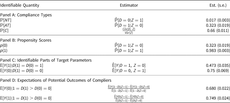
Note: Sample size =3023. This table presents other identifiable quantities in Kern and Hainmueller (Reference Kern and Hainmueller2009), namely, proportion of different compliance types, propensity scores, expectation of potential outcomes among compliers, and identifiable parts of target parameters. ${\mathbb P}[ NT]$ , ${\mathbb P}[ AT]$
 , and ${\mathbb P}[ C]$
 refers to the proportion of never-takers, always-takers, and compliers, respectively.
There are two interesting findings from Table 2. First, only $1.7\%$ of East Germans would not have watched Western media even if they had improved access to television signals. Second, the never-takers’ support rate for communism is high, $75\%$
 support communism. By comparison, only $47.3\%$
 of always-takers support communism.
4.3 Extrapolation 1: point estimates by linearizing MTR pairs
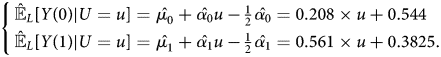
Recall proposition 1, if we impose linearity assumption on the MTR pairs, then, the ATEs of always-takers and never-takers are point identifiable. Under the linearity assumptions, it can be shown that for ${\mathbb E}_{L}[ Y \vert P( Z) = p,\; \, D = j]$ , where j ∈ {0, 1}, we have:
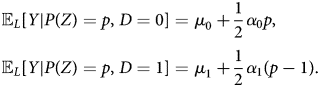
The quantities μ 0, α 0, μ 1, and α 1 are unknown. We can use sample analog of ${\mathbb E}[ Y \vert P( Z) = p( z) ,\; \, D = d] $ , with d ∈ {0, 1}, to solve the two linear equations below to compute $\hat {\mu }_{0}$
 , $\hat {\alpha }_{0}$
 , $\hat {\mu }_{1}$
 , and $\hat {\alpha }_{1}$
 :
:
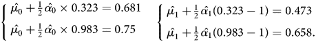
After solving the two equations, we have $\hat {\mu _{0}} = 0.648$ , $\hat {\alpha _{0}} = 0.208$
 , $\hat {\mu _{1}} = 0.663$
 , and $\hat {\alpha _{1}} = 0.561$
 . Then, the approximated MTR pairs based on linearity assumptions are:
Therefore, based on linearity assumptions, the extrapolated ATE of always-takers is:
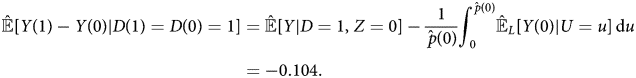
The extrapolated ATE of never-takers is:
These estimates show that the causal effect of media on attitudes depends on their propensity to consume the media. The ATE of always-takers is negative, meaning exposure to West German TV would make respondents less supportive of communism. By contrast, the ATE of never-takers is positive, reducing exposure to West German TV would make them less supportive of communism. For never-takers, the estimates support the “spiritual opium” hypothesis of Kern and Hainmueller (Reference Kern and Hainmueller2009)–perhaps watching West German TV makes their life more tolerable, increasing support for the government's preferred ideology. For always-takers, however, respondents are self-selecting the media sources according to their initial ideological positions.
The benefit of these estimates is that we can more directly speak to issues of political concern, such as the net effect of Western media exposure on support for communist ideology. We conduct a numerical experiment to compute this overall effect in the case of West German TV, taking into account the populations of compliers and the other two unobserved principal strata. In our numerical experiment, we compute the support rate of communism in two scenarios: when T = 1, i.e., when everyone consumes West German TV; when T = 0, i.e., when no one consumes West German TV. In the first scenario, we need to know following three quantities: $\hat {\mathbb {\mathbb E}}[ Y( 1) \vert D( 1) = D( 0) = 1]$ , $\hat {\mathbb {\mathbb E}}[ Y( 1) \vert D( 1) > D( 0) ]$
 and $\hat {\mathbb {\mathbb E}}[ Y( 1) \vert D( 1) = D( 0) = 0]$
 . In the second scenarios, we need to know: $\hat {\mathbb {\mathbb E}}[ Y( 0) \vert D( 1) = D( 0) = 1]$
 , $\hat {\mathbb {\mathbb E}}[ Y( 0) \vert D( 1) > D( 0) ]$
 and $\hat {\mathbb {\mathbb E}}[ Y( 0) \vert D( 1) = D( 0) = 0]$
 . Each of these quantities can be found in Table 2.
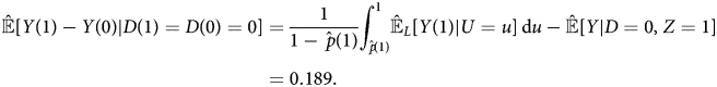
The overall effect of West German TV is summarized in Table 3. These results show that exposing the entire population to West German television would, on average, produce a small increase in support for communism. The average support rate for communism when no one consumes West German TV and when everyone consumes West German TV is $64.79\%$ and $66.3\%$
 respectively. However, Table 3 also shows that attitudes would be more polarized if everyone were exposed to West German TV.
Table 3. Effect of West German TV on Support for Communism
Note: Sample size = 3023. This table shows the support rate for communism under two hypothetical scenarios: either all residents in East Germany do not watch West German TV or they all do. In each cell in fourth and fifth rows, we calculate the support rate for communism across different types of residents.
4.4 Extrapolation 2: bounds by linear programming
The point estimation results require strong parametric assumptions on MTR pairs, possibly introducing severe misspecification bias. Our next step applies the linear programing approach to partially identify our target parameters, i.e., bound the ATEs of always-takers and never-takers.
The estimation of linear programing-based bounds involves inserting the sample analog into the estimating equation. The resulting maximization problem reduces to the following linear program:

A similar formulation is possible for the minimization problem.Footnote 11
There are two ways of proceeding with the extrapolation task. First, we can treat the ATEs of always-takers and never-takers as generalized LATEs, as both are weighted average of MTEs. Second, we can extrapolate the unknown part of our target parameters: $\hat {{\mathbb E}}[ Y( 0) \vert D( 1) = \;D( 0) = 1]$ and $\hat {{\mathbb E}}[ Y( 1) \vert D( 1) = D( 0) = 0]$
 , then, construct the bounds from the known parts of our target parameters. We present the results using the approach treating the ATEs of always-takers and never-takers as generalized LATEs.
The extrapolation results are presented in Figure 2. The x-axis depicts the polynomial order of the basis function used in the linear programing extrapolation. The y-axis displays the estimated ATE, controlling for each respondent's mother's occupation.Footnote 12 Each line shows the upper and lower bound for the extrapolation to each group. There two main conclusions. First, for never-takers, the bounds expand as we impose fewer restrictions on the basis functions. For always-takers, the estimated bounds are robust to difference choices of the basis functions. Second, Figure 2(b) show that the proportion of never-takers in our sample is too small to produce informative bounds. However, for always-takers, as shown in Figure 2(a), the bounds are sufficiently narrow to offer substantive insights.Footnote 13
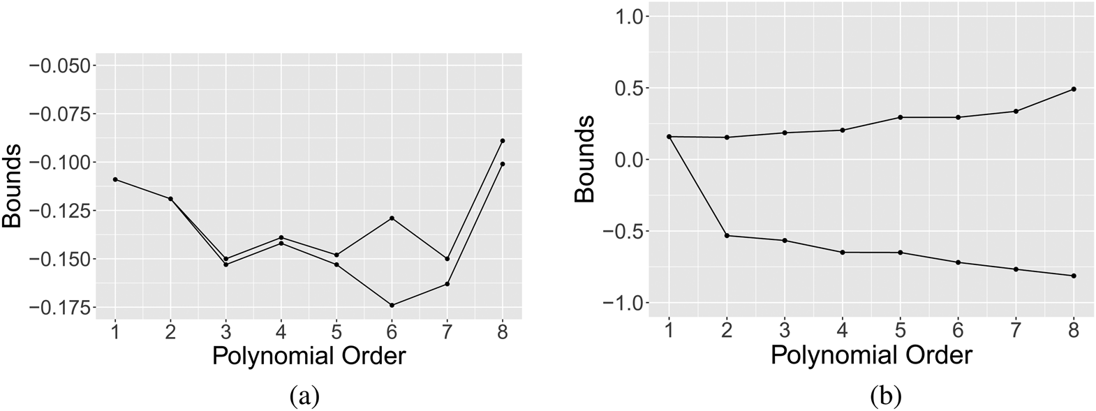
Figure 2. Extrapolate ATEs of always-takers and never-takers by linear programing. (a) ATE of always-takers: Generalized LATE. (b) ATE of never-takers: Generalized LATE. Note: Sample size =3023. This figure presents the bounds on the ATEs of always-takers and never-takers when we control mother's occupation in the linear program. The constraints in the linear program are the cross-moments in proposition C.1. The x-axis displays the polynomial order of the basis functions used in the linear program. Figures 2a,b are computed from treating ATEs of always-takers and never-takers as generalized LATEs in the linear program.
The results of extrapolation from the linear program show that there is a negative effect from West German TV on always-takers’ support for communism. Note that always-takers have the highest propensity to consume the West German's media. Therefore, one interpretation is that the always-takers are acting as-if they have anticipated the negative effects and self-select to consume the West German TV that reinforces their prior opposition to communism.
Moreover, we also provide empirical results from competing partial identification strategies in Appendix J. There are two main conclusions. First, some existing partial identification strategies produce bounds for the target parameters that are too wide to be informative. Second, there is a trade-off between the strength of assumptions and the widths of bounds, that is, researchers need to invoke stronger assumptions to get narrower bounds.
5. Conclusion
In many political settings, even under repressive conditions, individuals have control over their consumption of information. Instrumental variable (IV) analysis analyzes encouragements which shift the decision of some part of the population. The question then becomes how relevant any IV estimate is for a particular social scientific context, and how to draw conclusions about the broader population who are not responsive to a given encouragement.
Understanding counterfactual causal effects of those who are not responsive to a given encouragement can be of both practical and theoretical importance. However, we require tools for extrapolation. To do so, we restate the IV model in Imbens and Angrist (Reference Imbens and Angrist1994) in the latent utility framework of Vytlacil (Reference Vytlacil2002). Given this framework, we can define quantities that can be used in the process of extrapolation, including the average treatment effect for individuals who are just indifferent between selecting into or out of treatment. This framework allows for flexible heterogeneity of treatment effects with respect to latent utility, and is directly connected to individual behavior.
The key advantage of the latent utility framework is that it draws connections between our statistical assumptions and our substantive theories. Many classic treatment effect parameters, say, ATE, ATT, ATU, LATE, can be understood as weighted average of MTE, and these weights are identifiable from the data. As a result, the latent utility approach allows researchers to examine the match between their identification assumptions and their social scientific theories.
Furthermore, we show that, under the linear programing approach developed in Mogstad et al. (Reference Mogstad, Santos and Torgovitsky2018), it is possible to flexibly incorporate both structural assumptions and the treatment effect parameters into the extrapolation estimates. The former should be motivated by substantive theory, the latter are already calculated by existing IV approaches. The result are informative bounds, consistent with both the information provided by IV estimates and social scientific assumptions about the MTE function.
Our application to Kern and Hainmueller (Reference Kern and Hainmueller2009) demonstrates the value of directly modeling non-compliance. Using the linear programing approach to extrapolate IV estimates, we first replicate the effect described in the study and its consequences for a large population of always-takers. For always-takers, watching West German TV reduces support for communism. If access to West German TV were made more costly, it would drive up support for the regime. Substantively the self-selection of this population into treatment suggests that individual consumption of media may be driven by individual expectations—always-takers act as if they know the effect of watching West German TV and thus self-select into watching it.
Acknowledgements
We thank James Bisbee, Christopher Blattman, Matthew Blackwell, Anthony Fowler, Scott Gehlbach, Justin Grimmer, Kosuke Imai, Zeren Li, Zhaotian Luo, Azeem Shaikh, Joshua Ka Chun Shea, Alexander Torgovitsky, Yiqing Xu, Xiliang Zhao and Xiang Zhou, as well as participants from conferences at APSA-2020, Harvard Applied Statistics Workshop, International Methods Colloquium, MPSA-2020, and Political Science Speaker Series for Chinese Scholars for a multitude of helpful comments. We also would like to thank Holger Kern and Jens Hainmueller for sharing their data.
Supplementary material
The supplementary material for this article can be found at https://doi.org/10.1017/psrm.2023.46.
To obtain replication material for this article, https://doi.org/10.7910/DVN/S1QAE2


 Open access