


Crossref Citations
This article has been cited by the following publications. This list is generated based on data provided by Crossref.
Gu, Diandian
Wylie, Jonathan J.
and
Stokes, Yvonne M.
2024.
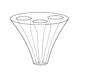
Drawing of fibres composed of shear-thinning or shear-thickening fluid with internal holes.
Journal of Fluid Mechanics,
Vol. 996,
Issue. ,