


1. Introduction
After the seminal study by Davies & Taylor (Reference Davies and Taylor1950), volumes of gas rising in a vertical tube are called Taylor bubbles when their equivalent spherical diameter is greater than the tube diameter. The buoyant rise of Taylor bubbles longer than a few tube diameters has the remarkable feature of occurring at a constant velocity independent of its length and, when viscous and surface tension effects can be neglected, only dependent on the acceleration of gravity and the tube diameter. It has been recognized that the flow taking place in the liquid film separating the gas from the tube wall, which D.D. Joseph called ‘drainage flow’ (Funada et al. Reference Funada, Joseph, Maehara and Yamashita2005), has a crucial importance in the bubble ascent. Continuity requires that the bubble rise at such a velocity that the volume flow rate of the drainage flow equals the volume per unit time vacated by the base of the rising bubble. Awareness of this fairly obvious fact is present in the earlier literature (see, e.g. Brown Reference Brown1965; Clanet, Héraud & Searby Reference Clanet, Héraud and Searby2004) without, however, drawing the conclusion that, by manipulating the film thickness so as to increase or decrease the drainage flow, it would be possible to affect the rising velocity of the bubble. In our earlier paper (Zhou & Prosperetti Reference Zhou and Prosperetti2021) we have shown by numerical simulation that, by constraining the bubble inside a porous cylinder coaxial with the tube, the drainage flow can be increased and the rising velocity correspondingly increased. A qualitative confirmation of this prediction has recently been obtained by Z. Zuo (personal communication 2023).
In this paper we demonstrate ways to decrease the drainage flow so as to markedly reduce the rising velocity of a Taylor bubble. We show that, by a subtle nonlinear process, a forced periodic variation of the bubble volume results in a thinning of the draining film that leads to this effect (§ 3). The effect is quite strong, with a marked slow down of the bubble occurring with volume pulsations of the order of a few percent.
As in our previous paper, our results are established by numerical means. We study a Taylor bubble rising in a vertical tube of finite length and consider two ways in which the bubble volume is caused to oscillate that we term kinematically and dynamically controlled. In the kinematically controlled oscillations the bubble volume is caused to pulsate by an imposed sinusoidal displacement of the top of the liquid column as could be produced, e.g. by a piston. The position  $Z_{top}$ of the top of the column is prescribed as
 \begin{equation} Z_{top}(t) ={-} A_t \cos \omega t , \end{equation}
in which  $A_t$ is the amplitude of the oscillations and
  $\omega$ their angular frequency. The
  $z$ axis, oriented upward, coincides with the axis of the tube and the top of the liquid column, when undisturbed, is located at
  $z=0$. With the dynamically controlled system, the liquid column has a free surface with mean position
  $z=0$ surmounted by a small gas space. The pressure
  $p(t)$ at the top of this gas region is prescribed by adding to the ambient pressure
  $p_a$ a sinusoidal oscillation with an amplitude of
  $\Delta P$ according to
 \begin{equation} p(t) = p_a +\Delta P\sin\omega t . \end{equation}
Due to their frequent occurrence in the chemical, energy and other industries, the literature on Taylor bubbles is quite voluminous, even pre-dating the study by Davies & Taylor (Dumitrescu Reference Dumitrescu1943). Important references on the subject are the papers by Bretherton (Reference Bretherton1961), Goldsmith & Mason (Reference Goldsmith and Mason1962), Polonsky, Shemer & Barnea (Reference Polonsky, Shemer and Barnea1999), Viana et al. (Reference Viana, Pardo, Yánez, Trallero and Joseph2003), Nogueira et al. (Reference Nogueira, Riethmuler, Campos and Pinto2006) and many others.
We can also point to a limited number of papers in which gravity-driven Taylor bubbles are affected by forced oscillations, although under a very different excitation compared with those considered here, namely by the forced vertical or horizontal oscillations of the vertical tube in which they rise. Kubie (Reference Kubie2000) studied horizontal oscillations of the tube finding a marked increase of the rising velocity that he explained as a consequence of the ‘effective acceleration’, given by the vector sum of gravity and the imposed acceleration. Although he did not discuss in detail the strong deformations of the bubble shape that he observed, it is evident from his images that they have the potential to greatly increase the drainage flow. In a short note, Brannock & Kubie (Reference Brannock and Kubie1996) reported experiments demonstrating the slowing down of a Taylor bubble in a vertically oscillating tube. Their work was continued and much extended by Madani, Caballina & Souhar (Reference Madani, Caballina and Souhar2009, Reference Madani, Caballina and Souhar2012) who, by gradually increasing the acceleration of the forced oscillations, documented an initial slowing down of the bubble rising followed by an increase at larger accelerations. Their attempt to explain these experimental results within the framework of an equation developed by Clanet et al. (Reference Clanet, Héraud and Searby2004), who adapted Davies & Taylor's original model based on an approximation of the flow in the nose region of a fixed-shape bubble, was not successful. In the end, they resorted to the development of correlations. Interestingly, both Brannock & Kubie and Madani et al. noticed a deformation of the bubble nose and, the latter, also waves propagating along the film surrounding the bubble but neither group followed up on these potentially interesting observations. Madani et al. (Reference Madani, Caballina and Souhar2009) mention an effect on the drainage flow as the bubble top expands and contracts without further elaboration.
The mechanism of the velocity reduction observed by both Brannock & Kubie and Madani et al. remains unexplained. An important difference with the situations studied in the present paper is that, in an oscillating tube, the oscillations are equivalent to an oscillating body force that permeates the entire liquid volume, above and below the bubble and in the film. On the other hand, in neither situation that we consider can pressure gradients develop along or under the bubble, a feature that will be seen to have a major effect. Another potentially important difference is that, since Madani et al.'s tube was closed (by releasing a stopper at the tube bottom, Brannock & Kubie, like Davies & Taylor, actually studied the emptying of the tube), their bubble had to maintain a constant volume while its volume is forced to oscillate in our study. It appears therefore that little can be learned from our study that has a bearing on the physics of a Taylor bubble in an oscillating tube without a separate investigation. For completeness, and in spite of the difference in scale and in the physics involved, we may also mention the volume oscillations of vapour Taylor bubbles in the pulsating heat pipes developed in recent decades (see, e.g. Nikolayev Reference Nikolayev2021; Su et al. Reference Su, Hu, Zheng, Wu, Liu, Zhu and Huang2023).
After a brief description of the numerical set-up and numerical method in § 2, we study the behaviour of the Taylor bubble under kinematically controlled oscillations in § 3, and under dynamically controlled oscillations in § 4. A summary and a few concluding considerations are presented in § 5.
2. Numerical set-up
The simulation is carried out with the compressibleInterFlow solver in the TwoPhaseFlow library developed by Scheufler & Roenby (Reference Scheufler and Roenby2023) based on the OpenFOAM framework. The solver directly simulates the Navier–Stokes equations allowing for compressibility effects and uses the volume-of-fluid method to deal with the gas–liquid interface. The plicRDF scheme is used for interface reconstruction; for more details, the reader can refer to Scheufler & Roenby (Reference Scheufler and Roenby2023). In the present paper we use the ideal-gas equation of state for the gas inside the bubble. Since, for the frequencies considered in this study, the wavelength of the pressure waves in the liquid far exceeds the length of the system we investigate, we assume the liquid to be incompressible with a constant density.
The flow is assumed to remain axisymmetric, thanks to which it is possible to simulate a thin wedge with two, rather than three, coordinates to reduce the computational burden. The mesh used in the simulations is orthogonal in both radial and vertical directions. With an aspect ratio close to 1, the cell size is gradually reduced towards the wall of the tube to have a better resolution of the velocity profile in the liquid film region. For most cases, we use 50 cells in the radial direction, although the terminal velocity of a normally rising Taylor bubble is predicted with a difference of less than 0.2 % by the use of 25 or 50 cells. The linearUpwind scheme is used for the convection terms of the momentum equation, whereas the vanLeer scheme is used for the advection of the volume-fraction field, both with second-order accuracy in space. We use the first-order implicit Euler scheme for the time discretization, which, after tests with the present highly unsteady flow field, has been found to be most stable among the available time stepping schemes.
The bubble is initially generated as a combination of a round cylinder and two hemispherical caps on each end of it. The initial film thickness is estimated according to the correlation provided in Llewellin et al. (Reference Llewellin, del Bello, Taddeucci, Scarlato and Lane2012). The no-slip condition is imposed at the tube walls. Figure 1 shows a comparison of our simulations of the rising velocity  $U_{B0}$ of a constant-volume, non-oscillating bubble (crosses) with some of the experimental data collected by Viana et al. (Reference Viana, Pardo, Yánez, Trallero and Joseph2003) (diamonds). A comparison with the theory of Brown (Reference Brown1965) is shown later in figure 11. The same computational tool has been used in several of our earlier papers where its accuracy is documented in greater detail (see, e.g. Zhou & Prosperetti Reference Zhou and Prosperetti2021, Reference Zhou and Prosperetti2022).

Figure 1. Comparison of the bubble rising velocity in the absence of excitation of the present simulation (purple crosses) with the experimental data collected in figure 9(c) of Viana et al. (Reference Viana, Pardo, Yánez, Trallero and Joseph2003) (blue diamonds). The upper cross is obtained with a Galilei number  $Ga$, defined in (2.3), of 73.71 used in the simulations presented in this paper; for the lower cross
  $Ga=36.86$. The range of Bond number (defined in (2.2a,b)) for the reference data is
  $14< Bo< 26$ while, in the present simulations, the Bond number has the fixed value 17.78.
The excitation of either type mentioned in § 1 is imposed after a transient stage during which the bubble reaches a steady shape and a constant rising velocity. Figure 2 shows schematics of the simulations and boundary conditions. In principle, for the kinematically controlled case, the displacement of the top of the liquid column renders the computational domain time dependent. We avoid the need for frequent gridding by imposing, in place of the displacement condition (1.1) at  $z=Z_{top}(t)$, the equivalent vertical velocity condition
 \begin{equation} u(z=0,t)= \omega A_t \sin \omega t , \end{equation}
where  $\omega A_t$ is seen to be the amplitude of the prescribed velocity oscillation. This condition is imposed at
  $z=0$ with a uniform profile over the tube cross-section. In order to avoid a conflict with the no-slip condition, wall slip is allowed over a short section of the tube close to the top boundary. The transition to a well-developed non-uniform velocity profile at deeper depths is found to be smooth. Since the region of the flow on which we focus is far below the top of the tube, this treatment has no influence on the dynamics of the Taylor bubble.

Figure 2. Schematic of the simulations for kinematically controlled oscillations in (a) (shown as driven by an oscillating piston) and dynamically controlled oscillations in (b).
In the kinematically controlled case, before the oscillation starts, the velocity at the top boundary is set to be zero to mimic a closed tube (or, as shown in figure 2(a), a stationary piston at  $z=0$). After the bubble has reached its equilibrium shape, we first slowly compress it by an amount
  $A_t$, then apply the velocity excitation (2.1) from this minimum-volume configuration. In this way, a gradual, instead of a sudden, start-up of the oscillation is achieved. The designation ‘kinematically controlled’ is motivated by the fact that the volume change of the bubble is solely determined by how much liquid is added or subtracted by the boundary condition (2.1), independently of the pressure in the bubble that changes passively during the oscillation.
For the dynamically controlled excitation, the oscillating pressure (1.2) is applied at the top of a small gas space occupying a height equal to two tube diameters above the liquid free surface as shown in figure 2(b). Due to the gradual decrease of the hydrostatic pressure, the bubble volume averaged over a period increases while it rises. For the deepest bubbles we have simulated (those shown in figure 17), the total amount of bubble expansion caused by this hydrostatic pressure change from its initial position to the free surface does not exceed 5 %, and is orders smaller within the distance corresponding to a single cycle of oscillation. Therefore, this effect is safely neglected in our subsequent discussion.
There are five parameters that are involved in the Taylor bubble motion in the absence of oscillations, i.e. the density  $\rho$ and viscosity
  $\mu$ of the liquid, the surface tension coefficient
  $\sigma$, the diameter of the tube
  $D$ and the gravitational acceleration
  $g$. The effect of the density and viscosity of the gas phase can be neglected in view of their typically much smaller values in comparison with those of ordinary liquids. According to dimensional analysis, two independent dimensionless groups can be constructed from the five independent parameters that we choose as the two commonly used ones in the study of the rise of bubbles, namely the Morton and Bond numbers, defined by
 \begin{equation} Mo = \frac{\mu^4g}{\rho \sigma^3},\quad Bo = \frac{\rho g D^2}{\sigma} . \end{equation}
Alternatively, one can use the Galilei number to replace either one of the above, i.e.
 \begin{equation} Ga = \frac{ \rho D \sqrt{g D}}{\mu} = \left(\frac{Bo^3}{Mo}\right)^{1/4} . \end{equation}
In the following we non-dimensionalize lengths by  $D$, times by
  $\sqrt {D/g}$ and pressures by
  $\rho g D$.
The code we have used also solves the energy equation in both phases that, in principle, would introduce a dependence on their thermal properties and, in particular, those of the gas. Since, as will be seen later, the bubble volume only executes small-amplitude oscillations, it can be assumed that the bubble pressure-volume relation is adequately described by a polytropic relation  $p_bV^\kappa \simeq {\rm const}.$, with
  $p_b$ the gas pressure in the bubble,
  $V$ its instantaneous volume and
  $\kappa$ a polytropic index. As shown in Chen & Prosperetti (Reference Chen and Prosperetti1998), this last quantity depends on the thermal penetration length into the gas, of the order of
  $\sqrt {D_{th}/\omega }$, with
  $D_{th}$ the gas thermal diffusivity. From the relations given in the reference, it can be estimated that, with a diatomic gas having the physical properties of nitrogen (which we used in the numerical simulation), in our case
  $1.3 < \kappa < \gamma$ with
  $\gamma =7/5=1.4$, the ratio of specific heats. Thus, in practice, in our simulations the gas can be considered to behave adiabatically and consideration of its thermal diffusivity becomes unnecessary. In other cases it may be necessary to account in greater detail for the gas thermal properties that, however, can always be reduced to a frequency-dependent polytropic index as shown in Chen & Prosperetti (Reference Chen and Prosperetti1998). In view of the large differences between the thermal capacities of the two phases, the liquid temperature changes by extremely small amounts that can be neglected to an excellent approximation.
The simulation of Taylor bubbles in low-viscosity liquids such as water involves problems such as unsteadiness of the bubble tail, loss of axisymmetry, small bubble shedding and turbulence, all hindering a focused analysis of the fundamental physics that we are interested in. For this reason, we use a Morton number of  $Mo=1.90 \times 10^{-4}$ that would correspond, for example, to a glycerol–water solution with
  $\mu =0.05076\ {\rm Pa}\ {\rm s}$,
  $\rho =1194.6\ {\rm kg}\ {\rm m}^{-3}$ and
  $\sigma =0.0659\ {\rm J}\ {\rm m}^{-2}$. For the Bond number, we have used
  $Bo = 17.78$ that, with the cited physical properties, would correspond to a tube diameter
  $D=10$ mm, very close to the 9.8 mm diameter one used by Madani et al. (Reference Madani, Caballina and Souhar2009, Reference Madani, Caballina and Souhar2012). With these physical properties and tube diameter, the Galilei number equals
  $Ga=73.71$. The flow remains laminar and the tail intact in most cases. In our simulations the bubble length at equilibrium is
  $L/D \approx 4$ with its volume
  $V_0/D^3\approx 1.8$, long enough for the liquid film around the bubble to be fully developed. The ambient pressure that is involved in the dynamically controlled case is
  $p_a/(\rho g D) = 864.6$, corresponding to the standard atmospheric pressure with the above dimensional values of
  $\rho$ and
  $D$.
$D$.
3. Kinematically controlled excitation
We start with the kinematically controlled excitation in which the top of the liquid column is forced to oscillate according to (1.1).
Figure 3(a) gives an overall picture of the shape of the bubble at different instants equally spaced during one period after steady-state oscillations have been reached; the dimensionless frequency is  $f\sqrt {D/g}=1.28$ with
  $f=\omega /2{\rm \pi}$,
  $D$ the tube diameter and
  $g$ the acceleration of gravity. The oscillation amplitudes are, from left to right,
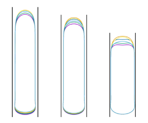
  $A_t/D = 0.025$, 0.05 and 0.09 and the corresponding variations of the bubble volume 1.1 %, 2.2 % and 4.0 %. There are several features worthy of notice. First, as expected, the amplitude of the nose oscillations increases as the driving amplitude increases. More interestingly, in spite of appearances, the undisturbed bubble volumes are the same in all three cases. Indeed, as the driving amplitude increases, a progressive thinning of the liquid film along the side of the bubble takes place with the consequence that the cross-section of the tube occupied by the gas increases and the bubble length shortens. Thirdly, the oscillations of the tail are imperceptible: all that can be seen is that it just moves monotonically upward. The amount of this upward motion during one period decreases with increasing drive from left to right, indicating a decreasing bubble rise velocity in the same order. Figure 3(b) shows the position versus time of the bubble nose (upper line) and tail (lower line) for the middle bubble of panel (a) with
  $A_t/D=0.05$. The relative insensitivity of the tail ascent to the imposed volume oscillations compared with the nose is quite evident. Because of this insensitivity, in the following we will use the period-averaged velocity of the bubble bottom,
  $U_B = \bar {U}_{bot}$, to quantify the bubble rising velocity when volume oscillations are present. The response of the liquid film to the imposed oscillations is not clear in figure 3(a). As will be shown presently, it is so small as to become noticeable only with a strong magnification. These observations reveal that the oscillations happen mainly in the bubble nose region, but can hardly penetrate the liquid film to reach the bubble tail. This point will be made clearer later.

Figure 3. (a) Evolution of shape and position of the rising Taylor bubble during one period for kinematically controlled oscillations. The vertical black lines are the wall of the tube. The driving frequency is  $f \sqrt {D/g}=1.28$ corresponding to a period
  $(2{\rm \pi} /\omega )\sqrt {g/D}\approx 0.78$. From left to right, the driving amplitude is
  $A_t/D=0.025$, 0.05 and 0.09. For each panel, six snapshots are taken at equal intervals of about 1/6th of a period after steady conditions have been reached. (b) Position versus time of the top and bottom of the middle bubble of panel (a).
The rising velocity of the bubble tail versus time for an ordinary, undisturbed Taylor bubble (dashed line) and the three cases of figure 3(a) are shown in figure 4. After steady conditions are reached with no forcing, oscillations start at  $t \sqrt {g/D}\approx 9.4$. There is a brief transient after which a steady regime is reached. The rising velocity then stabilizes around a steady value that decreases as the drive increases from top to bottom. It is quite remarkable that, for the largest amplitude
  $A_t/D=0.09$, corresponding to volume oscillations of about 4.0 %, the bubble slows down to a nearly vanishing velocity. This phenomenon is due to the unexpected fact that the oscillations cause the liquid film to become thinner than for an ordinary Taylor bubble with the consequence that the drainage flow decreases and so does the bubble rising velocity.

Figure 4. Bubble tail velocity  $U_B$, averaged over one oscillation period, as a function of time for the kinematically driven case. The frequency is
  $f\sqrt {D/g} = 1.28$ and the solid lines, from top to bottom, are for the oscillation amplitudes of
  $A_t/D=0.025$, 0.05 and 0.09. The excitation starts at
  $t \sqrt {g/D} \approx 9.4$. The dashed horizontal line is the velocity in the absence of oscillations.
3.1. Thinning of the liquid film
The key to an understanding of these results is the transient process by which the liquid film achieves the final thickness starting from the initial, larger undisturbed one. The explanation must start with the recognition that, except near the bubble top, the drainage flow in the film around the bubble is essentially governed by a balance of gravity and viscous effects (possibly augmented by turbulent dissipation when viscous effects are smaller) irrespective of the pressure imposed by the bubble on the film. Indeed, since the gas pressure in the bubble is very nearly uniform, no pressure gradients can arise to thin the film when the pressure rises or thicken it when it falls. Any such effect can only originate near the top of the bubble, because it is only in this region that pressure gradients can be developed to increase or decrease the film volume flow rate. The conclusion that, in the fully developed region, the film flow cannot be influenced by the pressure in the bubble can also be deduced from the very nearly parallel nature of the film flow in this region (possibly in a time-average sense with turbulence) and (by an argument similar to that of the boundary layer theory) from the separation of scales between the film thickness and the bubble length that makes the pressure in the film equal to that outside it, i.e. in the bubble. The fact that the film flow is purely gravity driven and not affected by the pressure variation in the top region largely prevents the bubble nose oscillations from influencing the flow in the tail region.
Let us focus in detail on the behaviour of the bubble shape in the initial stage of oscillation shown in figure 5(a). In order to highlight the important features of this result the image is highly distorted by a strong magnification of the horizontal scale. Note also that the image focuses only on a small radial range: neither the region near the axis of the tube, located at  $r=0$, nor that near the tube wall, located at
  $r/D=\frac {1}{2}$, are shown. The vertical dashed line indicates the position of the film surface before the start of the oscillations. The time ordering of the bubble outlines is the same as their ordering from bottom to top at the bubble tail. The first profile (green) is taken at maximum compression, the second and third ones (yellow and light blue) during the following expansion, the fourth and fifth ones (orange and purple) during the subsequent compression and the last one (dark blue) again at maximum compression. The bubble shape corresponding to the maximum expansion rate is shown without distortion in figure 5(b) where the small circle shows the position of the horizontal dashed line in panel (a).

Figure 5. (a) Six snapshots of the bubble surface during the second oscillation cycle starting with the expansion half-cycle (in order, the green, yellow, light blue lines) and concluding with the compression half-cycle (orange, purple and dark blue lines). Here  $f \sqrt { D/g} = 1.28$ and
  $A_t / D = 0.05$. The vertical dashed line shows the steady position of the side bubble surface before the oscillations start. (b) Flow field near the top of the bubble at the instant when the expansion rate reaches the maximum value and the bubble volume is at equilibrium, between the second and third lines (yellow and light blue) in panel (a). The vertical dashed and solid lines are the axis and the wall of the tube, respectively. The instantaneous streamlines and liquid velocity vectors in the laboratory frame are shown by white lines and (red) arrows (the corresponding information in the gas is irrelevant and is not shown for clarity). The small circle, located at the same depth as the horizontal dashed line in panel (a), marks the position at which the sideways enlargement of the bubble surface is greatest.
Each line in figure 5(a) shows two sideways enlargements of the bubble shape, one near the top and one near the bottom. The latter one is a standard feature of Taylor bubbles when inertia is prevalent or, at any rate, not insignificant (see, e.g. Magnini et al. Reference Magnini, Ferrari, Thome and Stone2017) and is not consequential for the present purposes. The important feature is the sideways enlargement near the bubble top. Also visible are sets of downward-propagating and damped capillary waves that would be expected to be induced by the strong deformation of the bubble top.
Consider the expansion half-cycle first (green, yellow and light blue lines). The bubble expands pushing some of the liquid upward while the liquid in the uniform region of the film continues to fall down under the action of gravity. Therefore, the vertical component of the velocity changes sign near the bubble nose, as demonstrated by the divergence of the streamlines in figure 5(b). A low-velocity region thus forms as indicated by the vanishing length of the velocity vectors. But the liquid in the lower film (near the small circle in figure 5b) drains continuously with its original downward velocity. As a result of volume conservation, the bubble surface must expand sideways as shown by the green, yellow and light blue lines in figure 5(a).
This mechanism can be better appreciated by comparing the streamlines shown in figure 6 for a non-oscillating (a) and oscillating (b,c) bubbles depicted in a frame of reference moving with the terminal velocity  $U_{B0}$ of the former. The snapshots for the oscillating cases are taken at the instant at which the expansion rate reaches the maximum and, therefore, the bubble length is the same as the equilibrium length. In this frame the non-oscillating bubble has a stagnation point at the nose with the liquid in free fall (if viscosity is disregarded) along the bubble surface as argued by Davies & Taylor (Reference Davies and Taylor1950) and as shown in figure 6(a). The flow in the film becomes fully developed (and the downward velocity stabilizes) when viscosity has permeated the entire film thickness. When the bubble expands as here, on the other hand, the nose must move upward so that the point where the vertical component of the velocity vanishes must be located at some distance under it (figure 6b,c). The liquid therefore has a shorter distance to fall and, at the same depth under the nose, its velocity will therefore be less. Lower down, however, the film flow rate cannot have changed for the reason explained before. Thus, the liquid supply is insufficient to maintain the film volume flow rate with the consequence that the film thins and the bubble enlarges sideways under the vertical velocity stagnation point during the expansion half-cycle as shown in figure 5. The distance by which this stagnation point descends is expected to be positively related to the strength of the expansion, which is quantified by the maximum liquid velocity
  $\omega A_t$ in (2.1). This correspondence can be checked by comparing the last two panels in figure 6. The lowering of the stagnation point decreases the velocity of the liquid by the time it reaches the uniform film region with the consequence that the film thinning effect is more significant.

Figure 6. Instantaneous streamlines in the frame of reference moving with the terminal velocity  $U_{B0}$ of an ordinary non-oscillating Taylor bubble. (a) At steady state without oscillation; (b,c) at the instant of the maximum rate of expansion during the first cycle of oscillation. The frequency is
  $f\sqrt {D/g}=1.28$. The amplitude
  $A_t/D$ is (b) 0.05 and (c) 0.025. The corresponding value of
  $\omega A_t /\sqrt {g D}$ is 0.40 and 0.20, respectively. The background colour shows the vertical component of the liquid velocity in the moving frame of reference adopted for this figure, and the small circles mark the points with zero value of it. The section of the bubble shown is about 1/6th of the entire length.
Owing to liquid inertia, at the end of the expansion, some time is needed for gravity to restore the fully developed film velocity and, in fact, for the cases in which the stagnation point is low enough, the low-velocity region can still be clearly observed in the compression half-cycle that follows. The flow velocity deficit persists therefore during at least a fraction of the compression in the course of which the film keeps thinning. Actually, if the frequency is high enough, the next expansion half-cycle will begin while the film thickness is still decreasing, as is the case in figure 5(a) (orange, purple and dark blue lines).
By the mechanism discussed above, the thinning of the film accumulates and propagates downward cycle after cycle until the film is so thin that the downward acceleration below the stagnation point is sufficient to maintain the much diminished volume flow rate (figure 7). The remarkable feature of the process is that the sideways enlargement taking place during one half-cycle is not cancelled by an opposite contraction during the next half-cycle. Rather, the effects of both half-cycles have the same sign and it is this circumstance that is responsible for the unexpected slowing down of the bubble.

Figure 7. The bubble surface every two periods (from bottom to top in time order) starting from the first instant when the oscillatory motion starts. Note the downward progress of the thinning of the liquid film from the top of the bubble. Here  $f\sqrt {D/g}=1.28$ and
  $A_t/D=0.05$. The vertical dashed line shows the steady position of the lateral surface of the bubble before the oscillations start.
The competition between inertia and velocity restoration is illustrated in figure 8(a), which shows the vertical velocity near the top of the bubble at three successive instants during the first compression half-cycle. The white arrows point to the region of low-velocity liquid straddling the film near the bubble nose. The strong interaction between the oscillation and the film flow shows the great potential for continuous film thinning. In contrast, the case in figure 8(b) has a smaller  $\omega A_t$. The stagnation point is thus closer to its original position without oscillation and the film flow is less blocked. It is seen that, with this lower amplitude, no appreciable low-velocity region can persist into the compression half-cycle so that the final steady film thickness has almost been reached. The same condition would also be seen for the case in figure 8(a), but only after a greater number of oscillation cycles, by which time the film would have become significantly thinner.

Figure 8. Distribution of the vertical velocity component during compression in the first oscillation cycle;  $T=2{\rm \pi} /\omega$ is the oscillation period. The amplitude of the oscillation is
  $A_t/D=0.075$ in (a) and 0.025 in (b). For both cases, the frequency of the oscillation is
  $f\sqrt {D/g}=1.28$. The arrows in panel (a) point to the area in the liquid film that is effectively blocked by low-velocity liquid.
The previous considerations suggest that a larger velocity oscillation amplitude  $\omega A_t$ leads to a thinner film thickness and, thus, a smaller bubble rising velocity. The effect of the driving amplitude
  $A_t$ with a fixed frequency
  $\omega$ has been shown in figure 4. It is expected that a similar effect would be observed if the frequency is varied with a fixed oscillation amplitude. This expectation is supported by the numerical results as can be seen in figure 9. In figure 9(a) the topmost straight line is the position versus time of the bottom of a Taylor bubble in the absence of oscillations. The other lines, from top to bottom, show the same quantity for progressively increasing frequency. These lines (except the straight one without imposed oscillations) exhibit some very small-amplitude oscillations that are all but invisible on the scale of the figure. The oscillations are somewhat clearer in panel (b), which shows the instantaneous velocity of the bubble bottom versus time for the same cases. Despite these oscillations, the decrease of the mean value of the bottom velocity shows a clear correlation to the increase of the driving frequency.

Figure 9. Time dependence of (a) depth and (b) instantaneous velocity of the bubble tail. The solid lines, from top to bottom, are for driving frequencies  $f\sqrt {D/g}=0.32$, 0.96, 1.28, 1.60 and 1.92, respectively. The amplitude is
  $A_t/D=0.05$ for all cases. The dashed lines show results without oscillations; excitation starts at
  $t\sqrt {g/D} \approx 9.4$.
The expected correspondence between decreased velocity and decreased film thickness can be checked in figure 10 that shows the film thickness  $h$ as a function of time. Similar to the bottom velocity shown in figure 9(b), the film thickness experiences oscillations that are more pronounced for low-frequency cases and rapidly decrease as the frequency is increased. These temporal oscillations correspond to a train of downward-propagating surface waves that are induced by the periodic deformation of the bubble nose. The variation of the film thickness caused by the waves is small (about 3 % for the blue line) and exactly cancels during one period. In any case, these waves do not have a significant effect on the phenomena we have described.

Figure 10. Time dependence of the film thickness measured close to the midpoint between the nose and tail of the bubble. From top to bottom, the solid lines correspond to frequencies  $f\sqrt {D/g}=0.32$, 0.96, 1.28, 1.60 and 1.92; the oscillation amplitude is
  $A_t/D=0.05$. The horizontal dashed line shows the film thickness in the absence of oscillations. The excitation starts at
  $t/\sqrt {g/D} \approx 9.4$.
3.2. Further considerations
Brown (Reference Brown1965) gives the following expression for the velocity profile  $u(r)$ in the steady, fully developed flow of a liquid film of thickness
  $h$ falling along the inner surface of a cylindrical tube of diameter
  $D$:
$D$:
 \begin{equation} u(r) ={-}\frac{\rho g}{8\mu}\left[\frac{1}{2}(D^2-4r^2)- (D-2h)^2 \ln \frac{D}{2r} \right]\!.\end{equation}
Here  $r$ is the radial distance from the tube axis. This expression is obtained from the steady Navier–Stokes equations with the assumption of parallel flow and the zero-stress condition at the gas–liquid interface. Upon combining this result with the condition of volume conservation, one can relate the bubble rising velocity
  $U_{B0}$ to the film thickness. The result accurate to the order of
  $O[(2 h/D)^4]$ is (Brown Reference Brown1965)
 \begin{equation} {U_{B0}}= \frac{\rho g D^2}{6\mu} \frac{ (2h/D)^3}{1-2h/D} . \end{equation}
We have found that, the expression (3.1) for  $u(r)$ well describes the velocity field in the fully developed flow region of our film at every instant irrespective of the bubble volume oscillations, which confirms that the drainage flow is in fact enslaved to the film thickness. We can therefore expect that (3.2), with
  $U_{B0}$ replaced by
  $U_B$, should also apply to our system. That this is indeed the case is shown in figure 11(a) in which the solid line represents (3.2) while the small circles mark the film thicknesses and the corresponding rising velocities obtained from the present simulations after the steady state is reached.

Figure 11. (a) The solid line is a graph of the Taylor bubble rising velocity as a function of the liquid film thickness  $h$ according to the result (3.2) of Brown (Reference Brown1965). The circles are the results of the present numerical simulations with driving frequencies, in decreasing order of
  $h$,
$h$,  $f\sqrt {D/g}=0$ (no oscillation), 0.32, 0.64, 0.96, 1.28, 1.60 and 1.92; the oscillation amplitude is
  $A_t/D=0.05$. The value of
  $h$ shown is averaged over one period of oscillation. (b) Position versus time of the bubble bottom when the oscillations are driven from below (wavy line) or from above (tilted purple line) the bubble; the dashed black line is the result without oscillations.
It is seen from figure 9 that the tail of the bubble is unaware of the oscillation (started at  $t\sqrt {g/D} \approx 9.4$) until
  $t\sqrt {g/D} \approx 13$. The time needed for the stabilization of the velocity of the tail increases with the driving frequency. With the largest frequency (the lowest line in figure 9b), the velocity reaches a constant value only after
  $t\sqrt {g/D} \approx 26$. The duration of the transient during which the film thins, and thus, the bubble rising velocity decreases, can be estimated by noting that flow-rate perturbations in a falling vertical film propagate with a velocity of the order of the Nusselt velocity,
  $u_{Nu} \approx h^2g/\nu$ with
  $\nu =\mu /\rho$ the liquid kinematic viscosity, a leading-order approximation of (3.1). If
  $L$ is the length of the bubble, the time taken for the film thickness variation at the top arriving at the tail of the bubble can be expected to be of the order of
  $L/u_{Nu}$ or
 \begin{equation} t\sqrt{\frac{g}{D}} = \frac{L\nu}{h^2\sqrt{gD}} = \frac{L_*}{h_*^2Ga} , \end{equation}
with  $L_*=L/D$,
  $h_*=h/D$ and
  $Ga$ the Galilei number defined in (2.3). The number of oscillation cycles corresponding to (3.3) is
  $L\omega \nu /(2{\rm \pi} h^2g)$.
For each driving frequency, the film thickness  $h$ changes from the original, undisturbed value
  $h_0$ to a terminal value at steady state
  $h_\infty$. Two different time scales can be obtained by substituting the two values of
  $h$ into (3.3). If
  $h_0$ is used, we get an estimate of the time within which the initial perturbation reaches the bubble tail, whereas the time within which the film thinning process has completed should be estimated with
  $h_\infty$, whose value depends on the driving frequency. With the data in figure 10 we find
  $t\sqrt {g/D} = 4.3$ by using
  $h_0$, and
  $t\sqrt {g/D} = 17.8$ by using
  $h_\infty$ for the slowest bubble (lowest line in figure 10). Both results agree well with our earlier observations in figure 9.
A confirmation of the importance of the drainage flow is provided by simulations in which the oscillations were driven from below the bubble while the top of the tube was closed. Some illustrative results are shown in figure 11(b) in which the dashed black line is the position of the bottom of a normal undisturbed Taylor bubble. The slightly oscillating line following it is the position of the bottom of the bubble in the presence of imposed oscillations from below. Since, with this arrangement, the drainage flow is not affected, the only difference between the two is due to the slight compression and expansion of the bubble caused by the imposed oscillations. The lowest, more inclined line is instead the position of the bubble bottom versus time when the oscillations are driven from the top at the same frequency. The huge difference between the rise velocity as obtained with the two oscillation drivers is an eloquent illustration of the role of the drainage flow.
In the previous considerations no mention has been made of the bubble length except for the derivation of (3.3). The reason is that, according to our explanation, the process of progressive film thinning proceeds downward with no upstream influence from the bubble tail back to the top. The difference to be expected with a longer bubble is only a longer transient in accordance with (3.3).
It would be useful if a correlation could be found to predict the bubble rising velocity. In the following we take a small step on this with fixed  $Mo$ and
  $Bo$, the definition and values of which have been provided in § 2. In this case, what can be controlled are the oscillation frequency
  $\omega = 2{\rm \pi} f$ and the velocity amplitude
  $\omega A_t$, both appearing in the boundary condition (2.1). Figure 12 shows the dependence of the steady-state bubble rising velocity
  $U_B$ on
  $\omega A_t$. The former is normalized by the terminal rising velocity
  $U_{B0}$ without volume oscillations. For each
  $\omega A_t$, five cases are simulated with the oscillation frequency
  $f\sqrt {D/g}$ ranging from 0.64 to 1.92 with equal intervals. The data points obtained with the same frequency are connected by dashed lines serving as guides to the eyes. The figure shows that, in the investigated parameter range,
  $\omega A_t$ plays a dominant role on the determination of the film thickness, and thus, the rising velocity, agreeing with the earlier discussion in this section. The oscillation frequency
  $f$ itself has a relatively minor influence. For a fixed value of
  $\omega A_t$, the rising velocity is smaller when
  $f$ is larger. The reason is two fold. First, with the same film thickness and position of the stagnation point, the low-frequency oscillation allows longer time for the recovery of the liquid velocity in the low-velocity region during the compression half-cycle. Therefore, the downward flow rate averaged over a period is larger, i.e. the film flow is less hindered. Secondly, for a fixed
  $\omega A_t$, a lower frequency
  $f=\omega /(2{\rm \pi} )$ means a larger oscillation amplitude
  $A_t$. If
  $A_t$ is so large as to be comparable to the length of the bubble nose, it is possible that, during compression, the top of the bubble is pushed much lower than the low-velocity region developed during expansion, whose influence on the film flow is therefore considerably weakened. It is worth pointing out that the data points would be significantly more scattered if the velocity ratio
  $U_B/U_{B0}$ were plotted as a function of the maximum acceleration
  $\omega ^2 A_t/g$, as suggested by Brannock & Kubie (Reference Brannock and Kubie1996) and others in their study of the Taylor bubble rising in a vertically oscillating tube.

Figure 12. Dependence of the steady-state bubble rising velocity on the oscillation amplitude of the liquid velocity, the former normalized by the terminal velocity of a rising Taylor bubble without volume oscillations. The data points connected by dashed lines are, from top to bottom, for oscillation frequencies  $f\sqrt {D/g}=0.64$, 0.96, 1.28, 1.60 and 1.92, respectively. The results for the three largest frequencies are close to each other and nearly overlap. The solid line is a fitted curve, (3.4), of the data on the lowest dashed line that are expected to be close to the asymptotic limit for large frequencies.
An intriguing feature of the numerical results shown in figure 12 is that, when the driving velocity amplitude  $\omega A_t$ is held constant, they suggest the existence of an asymptotic behaviour as
  $f\sqrt {D/g}$ increases. In the parameter range that we have investigated, the data for the largest value of this quantity,
  $f\sqrt {D/g}=1.92$, appear to be close to this asymptote that can be fitted very well by the expression
 \begin{equation} \frac{U_B}{U_{B0}} = \exp\left[{-}4.11 \left( \frac{\omega A_t}{\sqrt{gD}} \right)^2 - 5.56 \left( \frac{\omega A_t}{\sqrt{gD}} \right)^4 \right]\!, \end{equation}
as is shown by the grey line in the figure. We emphasize again that (3.4) is obtained with specific Morton and Bond numbers. A potentially interesting fact is that the constant 4.11 is close to  $\sqrt {Bo} = 4.22$ or
  $Ga/Bo=4.15$.
Equation (3.4) may shed some light on the nonlinear characteristics of the problem being discussed. With fixed driving frequency  $\omega$, the Taylor expansion of (3.4) for small driving amplitude
  $A_t$ yields
 \begin{equation} \frac{\Delta U_B}{U_{B0}} = \frac{U_{B0}-U_B}{U_{B0}} = 4.11 \left( \frac{\omega A_t}{\sqrt{g D}} \right)^2 + O\left[ \left( \frac{\omega A_t}{\sqrt{g D}} \right)^4 \right]\!, \end{equation}
confirming that the velocity reduction  $\Delta U_B$ depends nonlinearly on
  $A_t$ as stated before.
At first sight, figure 12, in which the results depend only weakly on  $f\sqrt {D/g}$, appears to be in contrast with figures 9(b) and 10, which exhibit a much stronger sensitivity to the value of the same parameter. In reality there is no conflict because changing
  $f$ and keeping
  $\omega A_t = 2{\rm \pi} f A_t$ constant in figure 12 requires changing
  $A_t$ in inverse proportion at the same time, while
  $A_t$ is kept constant in figures 9(b) and 10 as
  $f$ is changed. Thus, the consequences of varying
  $f\sqrt {D/g}$ in the two cases cannot be compared.
An obvious question is whether the slow down of the bubble that we have described can be pushed so far as to stop it altogether. It is known that, in small tubes, surface tension can have such a strong effect as to thin the film surrounding the bubble to the point that it breaks by van der Waals effects and a three-phase contact line forms. In this case the bubble cannot rise but remains frozen in place (Zukoski Reference Zukoski1966; Lamstaes & Eggers Reference Lamstaes and Eggers2017). Perhaps this limit can be reached by the present method although the matter cannot be pursued numerically because of difficulties with bubble stability and multi-scale requirements. If a three-phase contact line forms and the tube is not so small that one can rely on surface tension to stabilize the upper liquid surface that formed the top of the Taylor bubble, it would be an interesting problem whether this surface can be dynamically stabilized by the liquid column oscillation with a mechanism similar to that demonstrated by Apffel et al. (Reference Apffel, Novkoski, Eddi and Fort2020), who were able to stabilize a suspended liquid mass over a gas layer in a vertically oscillating container.
4. Dynamically controlled excitation
For the case of dynamically controlled excitation, illustrated in figure 2(b), the liquid column above the Taylor bubble has a free surface at its top. The pressure of the gas above this free surface oscillates sinusoidally according to (1.2). This configuration imposes a boundary condition on the force acting on the liquid column rather than on its displacement. Therefore, the dynamics of the liquid column as affected by its interaction with the bubble is expected to play a role in the determination of the bubble oscillations as well as its rising velocity.
The upper group of lines in the two panels of figure 13 show the time dependence of the bubble nose depth for different pressure amplitudes and  $f\sqrt {D/g}=1.28$ in panel (a) and 1.52 in panel (b). The lower groups of lines convey the same information for the bubble tail. The straight, inclined topmost line in each group is for a normal steadily rising Taylor bubble with the same undisturbed volume but without pressure excitation. The simulation starts at
  $t=0$ with the simplified bubble shape described in § 2. The oscillations start at
  $t\sqrt {g/D} \simeq 9.4$, by which time the shape of the bubble has relaxed to steady conditions.

Figure 13. Time dependence of the depth of the bubble nose (top group of lines in each panel) and tail (bottom group of lines) with a driving frequency  $f\sqrt {D/g}=1.28$ in (a) and 1.52 in (b) for dynamically controlled oscillations. In (a) the driving pressure amplitudes are, from top to bottom,
  $\Delta p/p_a=0$ (no oscillation), 0.004, 0.006 and 0.008 and in (b)
  $\Delta p/p_a=0$, 0.004, 0.005 and 0.006. The horizontal dashed lines roughly mark the position of the inflection points on the curves for the motion of the bubble top.
The slope of these lines decreases shortly after the start of the oscillations indicating a slower rising velocity. For the weaker excitations, the slope eventually returns to the original value, equal to that of an ordinary Taylor bubble. The same behaviour would be observed in all cases if the bubbles were to rise further. Therefore, an inflection point at which the second-order derivative of the curves changes sign from negative to positive can be found in each deceleration–acceleration process. In each panel of figure 13, the inflection points are located at approximately the same depth of the bubble top, marked by the dashed horizontal lines. The values of this critical depth, however, are different for the two different driving frequencies. Thus, unlike the kinematically controlled case of § 3, now the slowing down is temporary and occurs when the bubble nose is in the neighbourhood of a well-defined, frequency-dependent depth. We show below that, at this depth, the oscillations of the bubble volume reach a maximum amplitude for a given driving frequency  $\omega$. We designate this depth as the resonant depth, although it should be stressed that it does not necessarily coincide with conditions such that the oscillations of the bubble are in resonance with the drive.
Appendix A describes a simplified theory for the oscillations of the bubble and the resonant depth. The main simplification is that the bubble rising is neglected in the development, which will be justified provided the oscillation period is sufficiently short; a quantification of this statement will be provided shortly. It is shown in Appendix A that, when viscous effects are unimportant, the resonant depth is given by
 \begin{equation} H_{R,inv} = \frac{\gamma p_a/(\rho L_e)}{\omega^2-\omega_\infty^2} \quad {\rm with}\ \omega_\infty^2=\frac{\gamma g}{L_e} . \end{equation}
Here  $p_a$ is the undisturbed pressure at the free surface and
 \begin{equation} L_e=\frac{V_0}{{\rm \pi} R^2} \end{equation}
is an effective equilibrium bubble length expressed in terms of the undisturbed bubble volume  $V_0$ (see Appendix A). Since the inviscid resonance frequency
  $\omega _{0,inv}$ of the bubble at a depth of
  $H$ is given by (see Appendix A)
 \begin{equation} \omega_{0,inv}^2 = \frac{\gamma p_a}{\rho H L_e}+\omega_\infty^2 , \end{equation}
it is seen that, when  $H=H_{R,inv}$,
  $\omega = \omega _{0,inv}$ so that the bubble is driven at resonance. This is the only case in which the bubble executes resonant oscillations at the resonant depth. It is also seen from both (4.1) and (4.3) that
  $\omega _\infty$ is the natural frequency of a very deep bubble. In (4.1) and in the rest of this section we have assumed that the bubble executes adiabatic oscillations writing
  $\gamma$, the ratio of the gas specific heats, in place of a more general polytropic index; we include some considerations on this point in Appendix A.
With viscosity, for a given  $\omega$, the bubble response reaches its maximum approximately at the depth (see Appendix A)
 \begin{equation} H_R = \frac{\gamma p_a}{\rho L_e} \frac{\alpha \omega^2 - \omega_\infty^2}{\left(\alpha \omega^2 - \omega_\infty^2\right)^2 + \beta^2 \omega^4} , \end{equation}
in which  $\alpha$ and
  $\beta$ are two parameters dependent on the combination
  $\nu /(\omega R^2)$; they are defined in (A12) and graphed in figure 19. The parameter
  $\nu /(\omega R^2)$ is the inverse of the square of the Womersley number
  $Wo= R\sqrt {\omega /\nu }$ that is often used to characterize the behaviour of pulsatile flows such as blood flow in arteries (see, e.g. Ku Reference Ku1997). For small values of
  $\nu /(\omega R^2)$,
  $\alpha$ and
  $\beta$ are approximately given by
 \begin{equation} \alpha \simeq 1 + \sqrt{\frac{2\nu}{\omega R^2}} = 1 + \frac{\sqrt{2}}{Wo} , \quad \beta \simeq \sqrt{\frac{2\nu}{\omega R^2}} = \frac{\sqrt{2}}{Wo} , \end{equation}
and, over the entire range of  $\nu /(\omega R^2)$,
  $1 \leqslant \alpha < 4/3$. It is evident that in the inviscid limit, in which
  $\alpha =1$ and
  $\beta =0$, (4.4) reduces to (4.1) given earlier.
Corresponding to the value  $H_R$ of the resonant depth, the bubble oscillation amplitude attains the value
 \begin{equation} \frac{|X_M|}{\Delta P} = \sqrt{(\alpha -\omega_\infty^2/\omega^2)^2+\beta^2} \frac{L_e}{\beta\gamma p_a} . \end{equation}
This is the maximum oscillation amplitude as a function of the bubble depth  $H$ for a fixed
  $\omega$, not as a function of the driving frequency
  $\omega$ for a fixed depth
  $H$. As can be seen from (A16), when the bubble is much deeper than
  $H_R$, the oscillation amplitude is small and its rise velocity will be close to that of an ordinary Taylor bubble. Conversely, when the bubble is much above
  $H_R$ and close to the surface, the slowing down of the ascent will depend on the amplitude of the drive that, being close to that of the bubble pressure, determines the film thickness.
Figure 14 shows the normalized resonant depth  $H_R/(p_a/\rho g)$ as a function of
  $\omega /\omega _\infty$; the curves are parametrized by the dissipation parameter
 \begin{equation} N = \frac{\nu}{\omega_\infty R^2} . \end{equation}
It is evident from (4.4) that  $H_R$ vanishes for
  $\omega ^2=\omega _\infty ^2/\alpha$, grows as
  $\omega$ increases from this value, reaches a maximum (which becomes progressively smaller with increasing dissipation), past which it starts to decrease with the eventual asymptotic trend
 \begin{equation} H_R \simeq \frac{\alpha}{\alpha^2+\beta^2} \frac{\gamma p_a}{\rho \omega^2L_e} . \end{equation}
Figure 14. Normalized resonant depth as a function of  $\omega /\omega _\infty$, with
  $\omega _\infty$ the infinite-depth resonant frequency defined in (4.1). From bottom to top, the solid lines correspond to the viscosity parameter defined in (4.7)
  $N= 2$, 0.5, 0.1 and 0.01. The dashed line is the inviscid result (4.1).
For any value of  $N$, below the maximum of
  $H_R$, there are two values of the frequency that result in the same resonance depth. If, in an application, there are specific reasons to desire a particular value of
  $H_R$, it is likely that the larger value would be of interest as, in this way, the bubble would reside in the resonance region for a greater number of periods, and with a larger oscillation amplitude as can be seen from (4.6), both allowing for a greater decrease of the drainage flow along its side and, therefore, for a greater slow down of its rising velocity.
The relation between the bubble nose velocity and the bubble depth (both averaged over a period) is depicted in figure 15 for three driving pressure amplitudes. For all amplitudes, the shape of the curves is the same, with rapid oscillations (caused by a slight change of the phase and amplitude at each depth) superimposed on a common trend that slowly decreases as the resonant depth is approached and then increases as it is passed. The minimum of the velocity gets smaller as the driving pressure is increased but its position (which is also indicated by the horizontal dashed line in figure 13b) remains approximately the same except for a small displacement to lower depths with increasing amplitude caused by weak nonlinear effects.

Figure 15. Velocity of the bubble top as a function of its depth, both averaged over one period. The residual oscillations on the curves are due to the fact that the phase and amplitude of the bubble oscillations keep changing with depth. The driving amplitudes are, from top to bottom,  $\Delta p/p_a=0.004$, 0.005 and 0.006. The driving frequency is fixed at
  $f\sqrt {D/g}=1.52$.
The explanation of this behaviour is that the oscillation amplitude of the bubble increases as the resonant depth  $H_R$ is approached so that the film along its surface becomes thinner as we have explained in the previous section; the converse happens as the bubble rises above
  $H_R$. A direct illustration of this mechanism is provided in figure 16 that shows, magnified in the same way as in earlier figures, the lateral surface of the bubble as it goes through the resonant depth. The succession of lines from the lowest (purple) to the highest (blue) corresponds to the successive positions of the bubble separated by 16 periods. As the resonant depth is approached, the film thins (purple and yellow) reaching a minimum thickness at the resonant depth (green). As the bubble rises further (orange and blue), the film thickens again. The thickness of the liquid film increases from nose to tail when the bubble approaches the resonant depth because the bubble never resides at the same depth long enough for the analog of the transient depicted in figure 7(b) to reach completion. For the converse reason, the film thickness decreases from nose to tail as the bubble leaves the resonant depth.

Figure 16. Shape and position of the lateral surface of the rising Taylor bubble at successive instants separated by 16 oscillation periods for dynamically controlled oscillations. The frequency of the pressure oscillations is  $f\sqrt {D/g}=1.28$ and the amplitude
  $\Delta p/p_a=0.006$.
The interval of depths over which one may expect the decrease and increase of the rising velocity shown in figure 15 depends on the width of the bubble resonance that, itself, depends on the degree of damping affecting the oscillations. The width  $\Delta H_R$ of the resonance at half-height is given by
 \begin{equation} \Delta H_R = \frac{2\sqrt{3} \beta \omega_\infty^2\omega^2}{(\alpha \omega^2-\omega_\infty^2)^2+\beta^2 \omega^4} \frac{p_a}{\rho g} , \end{equation}
and is seen to be an increasing function of the damping parameter for  $\beta$ not too large. On substitution of the parameters, (4.9) predicts
  $\Delta H_R/D \approx 2.0$ for the case shown in figure 15, in good agreement with the simulation results. With this result we can now be more quantitative about the error introduced with the neglect of the bubble rise in the theory developed in Appendix A: the error can be expected to be small when the rise during one period, of the order of
  $2{\rm \pi} U_B/\omega$, with
  $U_B$ the bubble rise velocity, is smaller than
  $\Delta H_R$. This condition is evidently satisfied in the examples of figure 15 with
  $2{\rm \pi} U_{B0}/(\omega \Delta H_R ) \approx 0.06$ (which would be smaller if the instantaneous
  $U_B$ is used instead of
  $U_{B0}$) and, since the rise velocity is slowed down as an effect of the oscillations, can be expected to be satisfied in many situations.
The oscillation amplitudes of the bubble volume induced by the pressure oscillations used in the previous examples are of the order of a few percent. This circumstance suggests the slowing down of the bubble could be extended to a larger range of depths by the simultaneous use of a combination of different frequencies. The results of this approach are demonstrated in figure 17. Panel (a) shows the simulated bubble rising velocity with dimensionless driving frequencies  $f\sqrt {D/g}= 0.6$, 0.75 and 1. Also plotted is the result obtained with all the three driving signals acting simultaneously. With the multi-frequency drive, at every depth the rising velocity reduction approximately equals the sum of those caused by the individual frequencies. In panel (b) the analytical oscillation amplitude of the bubble predicted by (A16) is plotted against the depth. The predicted shape of all the curves has a good agreement with those in panel (a), reflecting a strong correlation between
  $\bar {U}_{top}$ and
  $|X|$ as was demonstrated in figure 12. At the maximum amplitude in panel (b), the volume variation is about 5 % of the equilibrium volume of the bubble for the largest single-frequency oscillation (purple), within the linear oscillation regime, reaching 8 % for the multi-frequency drive.

Figure 17. The top panel shows the dependence of the period-averaged bubble top velocity on its period-averaged depth, obtained from the numerical simulation. The three single-peaked curves, from left to right, correspond to pressure oscillation frequencies  $f\sqrt {D/g}= 0.6$, 0.75 and 1; the driving amplitude is
  $\Delta p/p_a=0.01$. The multi-peaked curve is the result with the simultaneous application of the three pressure oscillations. The horizontal grey line shows the rising velocity without oscillations. The black dashed line is obtained by algebraically adding the velocity reduction (compared with the grey line) of the three single-peaked results. The bottom panel, sharing the same horizontal axis with the top one, shows the theoretical result of the bubble oscillation amplitude
  $|X|$ calculated with the parameters corresponding to the three single-peaked cases in the top panel. The sum of the three curves is also shown. In the theoretical calculation, the polytropic indices are estimated with the method given by Chen & Prosperetti (Reference Chen and Prosperetti1998) and range from 1.314 to 1.333.
5. Summary and conclusions
A Taylor bubble rising in a tube slows down when it is subjected to small-amplitude forced volume oscillations because they diminish the drainage flow along its surface. During the expansion of the bubble, the film thickness decreases because of the imbalanced inflow and outflow in the film region, which is the result of the upward motion of the bubble nose. During contraction, it takes time for the drainage flow to re-establish itself, thus, the imbalance still exists and the film keeps thinning. As a consequence, the flow rate through the film is reduced in both half-cycles. Since the rise of the bubble is predicated on the ability of the drainage flow to replenish the space vacated by the rising bubble bottom, a slowing down of the drainage flow inevitably results in a slowing down of the bubble.
We have considered two different ways in which the bubble oscillations can be forced by acting on the liquid level at the top of the tube, an imposed displacement of the level (kinematic control) and an imposed pressure variation (dynamic control). With the first method, the bubble slow down persists over its entire ascent. With the second one, the slowing down is noticeable only while the bubble traverses a section of the tube centred at a depth at which the oscillations of the liquid column above the bubble are at a maximum. An alternative possible implementation would be a flexible tube section the diameter of which is made to vary periodically in time, with the top of the tube either open with a constant ambient pressure or closed.
For practical applications the stability of the bubble is important, an aspect of the problem that we have not examined in detail. However, we have found in our simulations that, in the kinematically driven case, if the imposed oscillations are stronger, namely,  $\omega A_t$ is larger than the data shown in figure 12, the shape of the bubble side surface may become irregular and solitary waves similar to those reported in Madani et al. (Reference Madani, Caballina and Souhar2009) appear. With even stronger oscillations, the nose of the bubble is destroyed by a combination of the Rayleigh–Taylor and Faraday instabilities as shown in figure 18. The appearance of liquid drops inside a Taylor bubble has been found before in other contexts (see, e.g. Andredaki et al. Reference Andredaki, Georgoulas, Miché and Marengo2021) but, in those cases, drops are formed by the folding of the bubble tail due to the increased pressure at the rear stagnation point rather than at the nose as here. The disruption of the bubble may go well beyond that shown in figure 18 as, depending on the driving amplitude, it is quite possible that the bubble would not remain intact as it passes through the resonant depth region. Conceivably, this might be a method to disrupt a bubble at a given depth.

Figure 18. Shape of a Taylor bubble with kinematically controlled oscillations imposed at the top of the tube. Three typical snapshots are selected in chronological order after the oscillation starts. The frequency is  $f\sqrt {D/g}=1.28$ and the amplitude
  $A_t/D=0.2$. In the third panel a droplet falls through the bubble. The thickness of the liquid film around the bubble near the top is close to zero.
We have also carried out a few numerical simulations with two or more Taylor bubbles finding that the varying pressure of the leading bubble operates on the trailing one similarly to the pressure drive of § 4. In this way the oscillations of the bubbles become coupled and the increased complexity of the situation does not permit a simple extrapolation of the single-bubble results of this paper.
Funding
G.Z. acknowledges the support of the National Natural Science Foundation of China (grant number 12202441) and the Fundamental Research Funds for the Central Universities.
Declaration of interests
The authors report no conflict of interest.
Appendix A. The resonant depth
It can be seen in figure 15 that the period of the driving for the bubble oscillations is much shorter than the time it takes the bubble to transit through the resonant depth region. This justifies an approximate model in which the bubble is considered to be at a fixed depth. Furthermore, in view of the smallness of the oscillations, the system composed by the bubble and the liquid column above it can be treated as a linear spring-mass oscillator. Beside the constant gravitational force, the liquid column is subjected to the pressure in the bubble,  $p_b$, and the disturbed pressure at the free surface, which it is convenient to write as
 \begin{equation} p(t) = p_a + \Delta P {\rm e}^{-{\rm i}\omega t} , \end{equation}
where i is the imaginary unit. The motion of the liquid column is represented by the displacement  $X$ of its mass centre. The governing equation for
  $X$ reads
 \begin{equation} \rho {\rm \pi}R^2 H \ddot X = {\rm \pi}R^2 (p_b - p) - \rho g {\rm \pi}R^2 H + 2 {\rm \pi}R H \tau_w , \end{equation}
where  $R$ is the tube radius,
  $H$ is the depth of the bubble measured at its top. The viscous shear stress at the wall,
  $\tau _w$, imposes damping on the system by dissipating some mechanical energy into heat.
It can be shown by elementary geometric considerations that with the assumption  $|X| \ll H$, the change
  $\delta V$ of the bubble volume can be expressed in terms of
  $X$ as
 \begin{equation} \frac{\delta V}{{\rm \pi} R^2} = X \left[ 1+O\left(\frac{X}{H}\right) \right]\!. \end{equation}
Assuming a pressure-volume relation for the gas governed by a polytropic index  $\kappa$ and confining ourselves to the linear approximation, justified when
  $|\delta V|/V_0 \ll 1$ with
  $V_0$ the undisturbed bubble volume, we write
 \begin{equation} p_b = \left(\frac{V_0}{V_0+\delta V}\right)^\kappa p_b^0 = \left(\frac{1}{1+X/L_e}\right)^\kappa p_b^0 \simeq \left(1- \frac{\kappa X}{L_e} \right)p_b^0 , \end{equation}
in which  $L_e$ is the equivalent bubble length defined in (4.2) and
  $p_b^0$ is the pressure inside the bubble at equilibrium, equal to the hydrostatic pressure at depth
  $H$, i.e.
 \begin{equation} p_b^0 = p_a + \rho g H . \end{equation}
We have neglected the pressure difference across the bubble interface due to the surface tension effect, which is at least an order smaller than the pressure variation caused by the volume oscillation in all of our cases.
In the linear approximation, in order to account for thermal dissipation, one can give an imaginary part to the polytropic index  $\kappa$ as explained in detail in Chen & Prosperetti (Reference Chen and Prosperetti1998). The effect is an augmentation of the damping coefficient
  $\beta$ introduced later. For simplicity, we assume that the bubble radius is much greater than the thermal penetration depth in the gas, so that
  $\omega R^2/D_{th} \gg 1$, with
  $D_{th}$ the gas thermal diffusivity. In this limit, thermal damping is negligible and
  $\kappa \simeq \gamma$, the ratio of the gas specific heats. On this basis we have written
  $\gamma$ in place of
  $\kappa$ in the equations of § 4 although we write
  $\kappa$ in this Appendix A as a reminder to the reader.
Upon substituting (A1), (A4) and (A5) into the equation of motion (A2) and neglecting for the moment  $\tau _w$, we find that
 \begin{equation} \ddot X + \omega_{0,inv}^2 X ={-} \frac{\Delta P}{\rho H} {\rm e}^{-{\rm i}\omega t} , \end{equation}
in which  $\omega _{0,inv}^2$ is the natural frequency in the absence of dissipation defined in (4.3) (with
  $\gamma$ replaced by
  $\kappa$). This expression for
  $\omega _{0,inv}$ can be found in Baird (Reference Baird1963) who was interested in the behaviour of a bubble in a vertically oscillating tube.
In order to account for  $\tau _w$, we note that the liquid column is ordinarily much longer than the tube diameter. This circumstance allows us to make the approximation of parallel flow for the entire liquid column, which leads to the Navier–Stokes momentum equation in the simplified form
 \begin{equation} \partial_t u ={-} \frac{1}{\rho} \partial_x p - g + \nu \left( \partial_r^2 u + \frac{1}{r} \partial_r u \right)\!, \end{equation}
where  $x$ is the coordinate along the tube axis pointing upward. By assuming
  $u \sim {\rm e}^{-{\rm i}\omega t}$ and using
  $\partial _x p = (p-p_b)/H$ justified by the fact that, as follows from (A7),
  $\partial _x^2 p=0$, noting (A1), (A4) and (A5), this equation becomes
 \begin{equation} \partial_r^2 u + \frac{1}{r} \partial_r u + {\rm i} \frac{\omega}{\nu} u = \frac{F(t)}{\nu} , \end{equation}
in which
 \begin{equation} F(t) = \frac{\Delta P}{\rho H} {\rm e}^{-{\rm i}\omega t} + \omega^2_{0,inv} X . \end{equation}
The solution regular at  $r=0$ and satisfying the no-slip boundary condition at
  $r=R$ is
 \begin{equation} u = \frac{{\rm i} F}{\omega} \left[ \frac{J_0(s)}{J_0(S)} - 1 \right], \quad {\rm with} \ s = r\sqrt{\frac{{\rm i}\omega}{\nu}} \quad \text{and} \quad S = R\sqrt{\frac{{\rm i}\omega}{\nu}}={\sqrt{{\rm i}} Wo} , \end{equation}
where  $Wo = R\sqrt {\omega /\nu }$ is the Womersley number. The wall shear stress readily follows as
  $\tau _w = [\mu \partial _r u]_{r=R}$ and the momentum equation (A2) may then be written as
 \begin{equation} \ddot{X} ={-} \left(1- 2 \frac{J_1(S)}{S J_0(S)} \right) \left( \omega_{0,inv}^2X+ \frac{\Delta P}{\rho H} {\rm e}^{-{\rm i}\omega t} \right)\!. \end{equation}
It is now convenient to introduce two real parameters  $\alpha$ and
  $\beta$ by
 \begin{equation} \alpha + {\rm i} \beta = \left(1 - 2 \frac{J_1(S)}{SJ_0(S)}\right)^{{-}1} . \end{equation}
The dependence of these parameters on the quantity  $\nu /(\omega R^2)={1/Wo^2}$ is shown in figure 19. The range of
  $\alpha$ is limited to the interval
  $[1,4/3)$;
  $\beta$, on the other hand, is large for small frequency and radius and large viscosity, all situations that increase the damping, and tends to zero as viscous effects become less significant. For the cases shown in this paper, the value of Wo ranges from 6 to 15.

Figure 19. Dependence of  $\alpha$ (purple line) and
  $\beta$ (green line) as defined in (A12) on the parameter
  $\nu /(\omega R^2)$. The horizontal dashed lines mark the asymptotic limits of
  $\alpha$ and
  $\beta$.
Since we are interested in steady solutions of the form  $X \sim {\rm e}^{-{\rm i} \omega t}$, we have the identities
  $\dot {X} = - {\rm i} \omega X$ and
  $\ddot {X} = - {\rm i} \omega \dot {X}$ from which the momentum equation (A11) can be recast into the standard form for a damped driven oscillator with all real coefficients,
 \begin{equation} \ddot{X} + \beta \omega \dot{X} + \left[ \omega_{0,inv}^2 - (\alpha - 1) \omega^2 \right] X ={-} \frac{\Delta P}{\rho H} {\rm e}^{-{\rm i} \omega t} , \end{equation}
from which the natural frequency  $\omega _0$ and damping
  $b$ of the oscillations can be read directly, i.e.
 \begin{equation} \omega_0^2 = \omega_{0,inv}^2 - (\alpha - 1) \omega^2 , \quad b = \tfrac{1}{2} \beta \omega . \end{equation}
The steady solution to (A13) is
 \begin{equation} X = \frac{\Delta P/(\rho H)}{\alpha \omega^2 - \omega_{0,inv}^2 + {\rm i} \beta \omega^2} {\rm e}^{-{\rm i} \omega t} , \end{equation}
from which the amplitude of the oscillations follows as
 \begin{equation} |X| = \frac{\Delta P/(\rho H)}{\sqrt{ \left(\alpha \omega^2 - \omega_{0,inv}^2 \right)^2 + \beta^2 \omega^4 } } . \end{equation}
The expression (4.4) for the resonance depth  $H_R$ is now found upon calculating the maximum of
  $|X|$ as a function of
  $H$ and the corresponding amplitude (4.6) upon substituting the result into (A16).


