Steady water waves with arbitrary surface pressure: their recovery from bottom-pressure measurements

Abstract

Equations relating the pressure at a horizontal seabed, the free-surface profile and the surface pressure are derived for two-dimensional irrotational steady water waves with arbitrary pressure at the free surface. Special cases include gravity, capillary, flexural and wind waves. Without approximations, we show that the free-surface recovery from the bottom pressure requires the resolution of only one first-order ordinary differential equation independent of the surface pressure, thus providing a new general recovery method valid for a broad class of water waves. Another equation provides an explicit expression for the surface pressure as a function of the bottom pressure and of the free surface. Thus, if unknown, the surface pressure can also be recovered if one extra measurement is available. This new recovery procedure is illustrated analytically for the linear approximation of a flexural–capillary–gravity wave, and numerically for fully nonlinear capillary–gravity waves.

1. Introduction

In this paper, we present equations relating the surface-wave profile, the surface pressure and the bottom pressure. This study includes any surface pressure describing various physical effects, such as capillarity, flexural elasticity, wind stress, etc.

Methods for recovering pure gravity (i.e. with constant pressure at the free surface) irrotational waves from bottom-pressure gauges have long been proposed. These methods solve the problem either exactly or under various simplifications; see Constantin (2012), Oliveras et al. (2012), Clamond & Constantin (2013), Vasan et al. (2017) and the references therein for reviews and details. Recently, Clamond, Labarbe & Henry (2023) showed that an exact recovery is also possible in the presence of constant vorticity. However, to the present authors’ knowledge, the recovery of capillary, flexural and wind waves (among many other situations of physical interest) has never been attempted. These phenomena involve different non-constant surface pressures that can be very complicated (especially for capillary and flexural waves), and the surface pressure is generally a function of the free-surface profile that is unknown a priori. Hence, compared with the case with constant surface pressure (i.e. pure gravity waves) treated in the references cited above, considering varying surface pressure is a major additional complication, requiring a new method of resolution for the wave recovery problem.

In this short paper, we describe a new general recovery method valid for any surface pressure. This is possible because the free-surface recovery from the bottom pressure requires the resolution of only one first-order ordinary differential equation independent of the surface pressure. Once known, the surface profile and the bottom pressure yield an explicit relation for the surface pressure. Thus, the surface profile and the surface pressure are both determined from the bottom pressure, but modulo an unknown scalar parameter (e.g. the Bernoulli constant), so one extra relation is required to close the problem. This can be obtained either by an extra measurement or by the knowledge of the physical effects at the free surface (i.e. knowing an equation the surface pressure must satisfy).

The paper is organised as follows. Section 2 is devoted to the physical assumptions and the resulting fundamental equations. Equations for the free-surface and the surface-pressure recovery from the bottom pressure are derived in § 3. The recovery procedure is illustrated analytically and numerically in § 4 and § 5, respectively. Finally, § 6 outlines some conclusions and perspectives.

2. Preliminaries

In the frame of reference moving with a travelling wave of permanent shape, the flow beneath the wave is a steady two-dimensional irrotational motion of an inviscid fluid. Note that the wave phase velocity $c$ is a non-zero constant in any other Galilean frame of reference. Let $(x,y)$ be a Cartesian coordinate system moving with the wave, $x$ being the horizontal coordinate and $y$ being the upward vertical one, and let $(u(x,y), v(x,y))$ be the velocity field in this moving frame of reference. We denote by $y=-d$, $y=\eta (x)$ and $y=0$ the equations at the bottom, the free surface and the mean water level, respectively. The latter equation expresses that $\langle \eta \rangle =0$ for a smooth $(2{\rm \pi} /k)$-periodic wave profile $\eta$, where $\langle {\cdot }\rangle$ is the Eulerian average operator over one period, i.e.

(2.1)\begin{equation} \left\langle \eta\right\rangle \stackrel{\text{{def}}}= \frac{k}{2{\rm \pi}} \int_{-{{\rm \pi}/k}}^{{{\rm \pi}/k}} \eta(x) \,\mathrm{d}\kern 0.06em x = 0. \end{equation}

For solitary and more general aperiodic waves, the same averaging operator applies taking the limit $k\to 0^+$.

The flow is governed by the balance between the restoring gravity force, the inertia of the system and a surface pressure. With constant density $\rho >0$ and acceleration due to gravity $g>0$ directed downward, the kinematic and dynamic equations are, for $(x,y)\in {\mathbb R}\times [-d,\eta (x)]$ (Wehausen & Laitone 1960),

(2.2a–d)\begin{align} u_x + v_y = 0, \quad v_x - u_y = 0, \quad uu_x + vu_y =-P_x/\rho, \quad uv_x + vv_y =- g-P_y/\rho , \end{align}

where $P(x,y)$ denotes the hydrodynamical pressure.

The flat bottom and steady free surface being impermeable, we have

(2.3a,b)\begin{equation} {v}_{b} = 0, \quad {v}_{s} = {u}_{s} \eta_x, \end{equation}

with $\eta _x\stackrel {\text {{def}}}=\,\mathrm {d}\eta /\mathrm {d} x$ and where subscripts ‘${b}$’ and ‘${s}$’ denote, respectively, restrictions at the bottom and at the free surface, e.g. ${u}_{b}(x)=u(x,-d)$, ${v}_{s}(x)=v(x,\eta (x))$. The pressure at the free surface is

(2.4)\begin{equation} {P}_{s} = P_{atm} + \rho {p}_{s}, \quad \text{at} \ y = \eta(x), \end{equation}

where $P_{atm}$ is a constant atmospheric pressure and ${p}_{s}$ is a varying pressure (divided by the density). For instance, one can consider a prescribed surface pressure such as a Gaussian distribution of magnitude $p_0$ and variance $\lambda$ (Wade et al. 2014),

(2.5)\begin{equation} {p}_{s} = p_0 \exp[-x^2/(2\lambda)], \end{equation}

or capillary and flexural effects such that (Lamb 1932; Toland 2008)

(2.6)\begin{equation} {p}_{s} =-\frac{\mathrm{d}}{\mathrm{d}\kern 0.06em x} \left\{ \frac{\tau\eta_x}{(1+\eta_x^{2})^{1/2}} - \frac{D\eta_{xxx}}{(1+\eta_x^{2})^{5/2}} + \frac{5D\eta_{x}\eta_{xx}^{2}}{2(1+\eta_x^{2})^{7/2}} \right\}, \end{equation}

with $\tau$ being a surface tension coefficient and $D$ a rigidity parameter (both divided by the fluid density). Other phenomena can of course be considered, as well as their combination. Without loss of generality, we take $\langle {p}_{s}\rangle =0$ since $\langle {p}_{s}\rangle$ can be absorbed into the definition of $P_{atm}$. It is thus convenient to introduce the normalised relative pressure

(2.7)\begin{equation} p(x,y) \stackrel{\text{{def}}}= [ P(x,y)-P_{atm}]/\rho, \quad (x,y)\in{\mathbb R}\times[-d,\eta(x)]. \end{equation}

The flow being irrotational, the dynamical (Euler) equations (2.2c,d) can be integrated into a Bernoulli equation:

(2.8)\begin{equation} 2 (\,p + gy) + u^2 + v^2 = B, \quad (x,y)\in{\mathbb R}\times[-d,\eta(x)] , \end{equation}

where $B$ is a Bernoulli constant. From (2.1)–(2.4) and (2.8), one gets (Clamond & Constantin 2013; Clamond et al. 2023)

(2.9)\begin{equation} B = \langle {u}_{s}^{2} + {v}_{s}^{2} \rangle = \langle {u}_{b}^{2} \rangle, \end{equation}

yielding the, here important, relation

(2.10)\begin{equation} \left\langle {p}_{b}\right\rangle = gd. \end{equation}

Finally, (2.2a,b) imply that the complex velocity $w\stackrel {\text {{def}}}= u-\mathrm {i} v$ is a holomorphic function of the complex coordinate $z\stackrel {\text {{def}}}= x+\mathrm {i} y$, an interesting feature exploited below.

3. Equations for the free-surface and surface-pressure recoveries

For free-surface and surface-pressure recoveries, we present here a simple derivation of equations generalising those of Clamond (2013) and Clamond & Constantin (2013).

3.1. General equations

The function $w^2$ being holomorphic, its real and imaginary parts satisfy the Cauchy–Riemann relations

(3.1a,b)\begin{equation} \partial_y(u^2-v^2) - \partial_x(2uv) = 0, \quad \partial_x(u^2-v^2) + \partial_y(2uv) = 0. \end{equation}

Integrating over the water column and using the boundary conditions, these relations yield after some elementary algebra

(3.2a,b)\begin{equation} {p}_{b} - {p}_{s} - gh = \frac{\mathrm{d}}{\mathrm{d}\kern 0.06em x} \int_{-d}^\eta uv \,\mathrm{d} y, \quad \left( {p}_{s} + g\eta \right) \frac{\mathrm{d}\eta}{\mathrm{d}\kern 0.06em x} = \frac{\mathrm{d}}{\mathrm{d}\kern 0.06em x} \int_{-d}^\eta \frac{u^2-v^2+B}{2} \,\mathrm{d} y. \end{equation}

Taylor expansions around $y=-d$ can be written (Lagrange 1781; Fenton 1972; Clamond 2022)

(3.3)$$\begin{gather} u^2 - v^2 = \cos [ (y+d) \partial_x ] {u}_{b}^{2} =-2 \cos[ (y+d) \partial_x] ({p}_{b} - gd), \end{gather}$$

(3.4)$$\begin{gather}2uv =-\sin[ (y+d) \partial_x ] {u}_{b}^{2} = 2 \sin[ (y+d) \partial_x ] ({p}_{b}-gd) \end{gather}$$

or in complex form

(3.5)\begin{equation} w(z)^2 = \exp[ \mathrm{i} (y+d) \partial_x ] {u}_{b}(x)^2 = {u}_{b}(z+\mathrm{i}d)^2 = B + 2gd - 2{p}_{b}(z+\mathrm{i}d). \end{equation}

(For any real function $F(x)$ continuable in the complex plane, $F(x+\mathrm {i} h)= \exp [ \mathrm {i} h \partial _x ]F(x)$ is the Taylor expansion around $h=0$.) Hence, with $h\stackrel{\text{{def}}}= d +\eta$, we have

(3.6a)$$\begin{gather} \int_{-d}^\eta uv\,\mathrm{d} y = \left[ 1 - \cos\left( h \partial_x \right) \right] \partial_x^{-1} \left({p}_{b} - gd\right)\!, \end{gather}$$

(3.6b)$$\begin{gather}\int_{-d}^\eta \frac{u^2-v^2+B}{2}\,\mathrm{d} y =-\sin\left( h \partial_x \right) \partial_x^{-1} ({p}_{b} - gd), \end{gather}$$

so (3.2) yield

(3.7)$$\begin{gather} {p}_{s} + g\eta = \partial_x \cos\left( h \partial_x \right) \partial_x^{-1} \left({p}_{b} - gd \right) = \left[ \cos\left( h \partial_x \right) - \eta_x \sin\left( h \partial_x \right) \right] ({p}_{b} - gd), \end{gather}$$

(3.8)$$\begin{gather}(B-{p}_{s}-g\eta) \eta_x = \partial_x \sin\left( h \partial_x \right) \partial_x^{-1} \left({p}_{b} - gd \right) = \left[ \sin\left( h \partial_x \right) + \eta_x \cos\left( h \partial_x \right) \right] ({p}_{b} - gd). \end{gather}$$

After one integration, (3.8) becomes

(3.9)\begin{equation} B\eta - {\textstyle{\frac{1}{2}}} g \eta^2 - \partial_x^{-1} \left( {p}_{s} \eta_x \right) = \sin\left( h \partial_x \right) \partial_x^{-1} ({p}_{b}-gd) . \end{equation}

With the special surface pressure (2.5) the term $\partial _x^{-1}{p}_{s} \eta _x$ cannot be obtained in closed form, but with (2.6) we have

(3.10)\begin{equation} \partial_x^{-1} ( {p}_{s} \eta_x) = \frac{\tau} {(1+\eta_x^{2})^{1/2}}-\tau + \frac{D \eta_x \eta_{xxx} - 3D \eta_{xx}^{2}}{(1+\eta_x^{2})^{5/2}} + \frac{5D \eta_{xx}^{2}}{2(1+\eta_x^{2})^{7/2}} + \text{constant}, \end{equation}

where the integration constant must be determined by the mean level condition (2.1), i.e. imposing

(3.11)\begin{equation} \big\langle {\textstyle{\frac{1}{2}}} g \eta^2 + \partial_x^{-1} ( {p}_{s} \eta_x) + \sin( h \partial_x) \partial_x^{-1} ({p}_{b} - gd) \big\rangle = 0 . \end{equation}

Note that the value of the integration constant in $\partial _x^{-1} ({p}_{b}-gd)$ does not matter here because this constant vanishes after application of the pseudo-differential operator $\sin ( h\partial _x )$.

Equations (3.7), (3.8) and (3.9) are generalisations for ${p}_{s}\neq 0$ of the relations derived by Clamond & Constantin (2013, equation (3.5)–(3.6)) and by Clamond (2013, equation (4.4)) when ${p}_{s}=0$. (This is obvious introducing the holomorphic function $\mathfrak {P}(z) \stackrel {\text {{def}}}= {p}_{b}(z+\mathrm{i}d )$ and $\mathfrak {Q}(z)\stackrel {\text {{def}}}= \int [\mathfrak {P}(z)-gd] \,\mathrm {d} z$.)

3.2. Generic equation for the free-surface recovery

When ${p}_{s}=0$ (pure gravity waves), $\eta$ can be obtained from ${p}_{b}$ solving the ordinary differential equation (3.8) (Clamond & Constantin 2013) or, more easily, solving the algebraic equation (3.9) (Clamond 2013). When ${p}_{s}\neq 0$ is a function of $x$ and/or $\eta$, such as (2.5) and (2.6), in general (3.9) is a complicated highly nonlinear high-order integro-differential equation for $\eta$ due to the term $\partial _x^{-1}( {p}_{s} \eta _x )$ (see relation (3.10) for an example of practical interest). This is not a problem for recovering the free surface $\eta$ from the bottom pressure ${p}_{b}$ because the surface pressure ${p}_{s}$ can be eliminated between (3.7) and (3.8), yielding

(3.12)\begin{equation} B \eta_x = [(1-\eta_x^{2}) \sin(h \partial_x ) + 2 \eta_x \cos( h \partial_x)] ({p}_{b} - gd), \end{equation}

or in complex form, introducing $\tilde {\mathfrak {P}}(z)\stackrel {\text {{def}}}= {p}_{b}(z+\mathrm{i}d )-g d$,

(3.13)\begin{equation} B \eta_x = ( 1-\eta_x^{2}) \operatorname{Im}\{ {\tilde{\mathfrak{P}}}_{s}\} + 2\eta_x \operatorname{Re}\{ {\tilde{\mathfrak{P}}}_{s}\} , \end{equation}

that is, a (nonlinear) first-order ordinary differential equation for $\eta$. Equation (3.13) being algebraically quadratic for $\eta _x$, it can be solved explicitly for $\eta _x$; thus one gets

(3.14)\begin{equation} \operatorname{Re}\{ {\tilde{\mathfrak{P}}}_{s}\} - \eta_x \operatorname{Im} \{ {\tilde{\mathfrak{P}}}_{s} \} = {\textstyle{\frac{1}{2}}} B \pm {\textstyle{\frac{1}{2}}} \vert B - 2 {\tilde{\mathfrak{P}}}_{s} \vert. \end{equation}

Since the free surface is flat if the bottom pressure is constant (and because $B>0$), the minus sign must be chosen. Moreover, the condition (2.9) rewritten in terms of $\tilde {\mathfrak {P}}$ yielding $B = \langle \vert B - 2 {\tilde {\mathfrak {P}}}_{s} \vert \rangle$, the average of the right-hand side of (3.14) is zero, so is the left-hand side.

Equation (3.14) is a priori not suitable if $\eta$ is (nearly) not differentiable (limiting waves). It is thus more efficient to solve its antiderivative

(3.15)\begin{equation} \operatorname{Re}\{ {\mathfrak{Q}}_{s} \} - K = {\textstyle{\frac{1}{2}}}\partial_x^{-1} (B-|B - 2 {\tilde{\mathfrak{P}}}_{s} |), \end{equation}

where $K$ is an integration constant and where $\mathfrak {Q}(z)\stackrel {\text {{def}}}= {q}_{b}(z+\mathrm{i}d )$, with ${q}_{b}(x)\stackrel {\text {{def}}}=\partial _x^{-1} ({p}_{b} -g d)$. Assuming $\langle {q}_{b}\rangle \stackrel {\text {{def}}}=0$ (without loss of generality), it yields $\partial _x\operatorname {Re}\{{\mathfrak {Q}}_{s}\} = \operatorname {Re}\{ {\tilde {\mathfrak {P}}}_{s} \} - \eta _x \operatorname {Im}\{ {\tilde {\mathfrak {P}}}_{s} \}$ and $\langle (1+\mathrm {i}\eta _x){\mathfrak {Q}}_{s}\rangle =0$. The right-hand side of (3.15) being the antiderivative of a zero-average quantity, we conveniently choose $\langle \partial _x^{-1} (B - \vert B - 2 {\tilde {\mathfrak {P}}}_{s} \vert ) \rangle \stackrel {\text {{def}}}=0$, hence $K = \langle \operatorname {Re}\{ {\mathfrak {Q}}_{s} \} \rangle$. Thus, a numerical resolution of (3.15) does not require the computation of $\eta _x$, which is an interesting feature for steep waves.

3.3. Recovery of the surface pressure

The free surface $\eta$ being obtained after the resolution of (3.14) or (3.15), the surface pressure ${p}_{s}$ is obtained explicitly at once from (3.7):

(3.16)\begin{equation} {p}_{s} = \partial_x \operatorname{Re}\{{\mathfrak{Q}}_{s}\} - g\eta = \operatorname{Re}\{ {\tilde{\mathfrak{P}}}_{s} \} - \eta_x \operatorname{Im}\{ {\tilde{\mathfrak{P}}}_{s} \} - g \eta. \end{equation}

Thus, as $\eta$, ${p}_{s}$ is known modulo the Bernoulli constant $B$. Relation (2.10) holds as a definition of the mean depth $d$, leaving us with only one scalar quantity to be determined (i.e. $B$).

3.4. Closure relation

In order to fully recover both the free surface and the surface pressure, knowing the bottom pressure is not sufficient and one extra piece of information is needed. We consider here two possibilities of practical interest.

A first possibility is when we have access to one independent extra measurement, for instance the mean velocity at the bottom (or elsewhere), the mean pressure somewhere above the seabed, the phase speed, the wave height, etc. In that case, the Bernoulli constant $B$ is chosen such that the recovered wave matches this measurement. Thus, the free surface and the surface pressure can be both fully recovered.

If no extra measurements are available (only the bottom pressure is known), the free surface can nevertheless be fully recovered with the knowledge of the physical nature of the surface pressure, for instance given by (2.5) or (2.6) (among many other possibilities). The missing parameter can then be obtained minimising an error (quadratic or minimax, for example) between the recovered surface pressure ${{p}_{s}}_r$ obtained from (3.16) and the theoretical surface pressure ${{p}_{s}}_t$ given, say, by (2.6).

3.5. Remarks

The fact ${p}_{s}$ can be eliminated is not surprising. Indeed, ${p}_{b}$ too can be eliminated between (3.7) and (3.8), yielding the equation

(3.17)\begin{equation} {p}_{s} + g\eta = \partial_x \cos( h\partial_x) \sin( h\partial_x )^{-1} [ B\eta - {\textstyle{\frac{1}{2}}} g\eta^2 - \partial_x^{-1}({p}_{s}\eta_x)], \end{equation}

or, after inversion of the pseudo-differential operator,

(3.18)\begin{equation} B\eta - {\textstyle{\frac{1}{2}}} g\eta^2 - \partial_x^{-1}\left({p}_{s}\eta_x\right) = \sin\left(h\partial_x\right)\cos\left( h\partial_x \right)^{-1} \partial_x^{-1} \left( {p}_{s} + g\eta \right)\!. \end{equation}

Relation (3.18) with ${p}_{s}=0$ is an Eulerian counterpart of the Babenko (1987) equation (Clamond 2018). A more involved Eulerian equation, somehow similar to (3.17) with ${p}_{s}=0$, was derived by Fenton (1972, equation (10)).

Note that, in its present form, (3.18) is not suitable for accurate numerical computations of $\eta$ due to the complicated pseudo-differential operator. For this purpose, its integral formulation is better suited (Clamond 2018, § 6). However, (3.17) and (3.18) are convenient to derive analytic approximations (cf. § 4 where surface recovery is performed analytically for linear flexural–capillary–gravity waves in order to illustrate the procedure).

4. Example 1: recovery of linear flexural–capillary–gravity waves

Here, we illustrate the recovery procedure for an infinitesimal flexural–capillary–gravity wave that is analytically tractable via its linear approximation.

4.1. Linear approximation of a travelling wave

For infinitesimal waves, the surface pressure (2.6) and the Babenko-like equation (3.17) are linearised as

(4.1a,b)\begin{equation} {p}_{s} \approx D \eta_{xxxx} - \tau \eta_{xx}, \quad {p}_{s} + g \eta \approx \partial_x \cos\left( d\partial_x \right) \sin\left( d\partial_x \right)^{-1} B \eta. \end{equation}

The $(2{\rm \pi} /k)$-periodic solutions are thus $\eta \approx a\cos (kx-\varphi )$ (a the constant amplitude with $ka\ll 1$ and $\varphi$ a constant phase shift) with the (linear) dispersion relation

(4.2)\begin{equation} B \approx (g + \tau k^2 + D k^4)k^{-1}\tanh(kd) . \end{equation}

The linear approximation of the bottom pressure can then be obtained as

(4.3a,b)\begin{align} {p}_{b} \approx gd + \mathfrak{p} \cos(kx-\varphi), \quad \mathfrak{p} = a ( g + \tau k^2 + D k^4) \operatorname{sech}(kd) = kaB \operatorname{csch}(kd), \end{align}

and the horizontal velocity at the bottom as

(4.4)\begin{equation} {u}_{b} \approx{\pm} \sqrt{B} [ 1 - B^{-1} \mathfrak{p} \cos(kx-\varphi) ]\quad\implies\quad \langle {u}_{b} \rangle \approx{\pm} \sqrt{B}. \end{equation}

This relation shows that, to this order of approximation, the Bernoulli constant $B$ can be replaced by $\langle {u}_{b}\rangle ^2$. Moreover, the sign of $\langle {u}_{b}\rangle$ gives the direction of propagation. Thus, in terms of parameters measurable at the bottom, the (linearised) free surface is

(4.5)\begin{equation} \eta \approx k^{-1} \left\langle {u}_{b} \right\rangle^{-2} \mathfrak{p} \sinh(kd)\cos(kx-\varphi). \end{equation}

4.2. Free-surface and surface-pressure recoveries

Suppose that data of the bottom pressure can be well approximated by the ansatz (4.3a). A least squares (for example) minimisation between the data and (4.3a) gives $gd$, $k$, $\varphi$ and $\mathfrak {p}$; these parameters are now definitely known. We have to the first-order in $\eta$

(4.6)$$\begin{gather} {\tilde{\mathfrak{P}}}_{s} \approx \mathfrak{p} \cos(kx-\varphi +\mathrm{i} kd) - \mathrm{i}\mathfrak{p}\sin(kx - \varphi + \mathrm{i} kd) k \eta, \end{gather}$$

(4.7)$$\begin{gather}{\mathfrak{Q}}_{s} \approx k^{-1} \mathfrak{p} \sin(kx - \varphi + \mathrm{i} kd) + \mathrm{i} \mathfrak{p} \cos(kx - \varphi - \mathrm{i} kd) \eta, \end{gather}$$

and, for infinitesimal waves, both $\mathfrak {p}$ and $\eta$ are small quantities of the same order. Thus, to the leading order, the recovery formula (3.14) yields

(4.8)\begin{equation} \mathfrak{p} \sinh(kd) \sin(kx - \varphi) + B \eta_x \approx 0 \quad\implies\quad \eta = (kB)^{-1} \mathfrak{p} \sinh(kd) \cos(kx-\varphi), \end{equation}

where the resolution is performed under the condition (2.1). Similarly, to the leading order, the relation (3.16) yields the surface pressure

(4.9)\begin{equation} {p}_{s} \approx [ \cosh(kd) - g(kB)^{-1} \sinh(kd) ] \mathfrak{p} \cos(kx-\varphi) = [ kB \coth(kd) - g] \eta. \end{equation}

With (4.8) and (4.9), the free surface and the surface pressure, respectively, are recovered modulo only one yet unknown parameter: the Bernoulli constant $B$. If, for instance, $\langle {u}_{b}\rangle$ has also been measured, then we have $B\approx \langle {u}_{b}\rangle ^2$ and the solution (4.5) is recovered. If no extra measurements are available, but if we know that we are dealing with flexural–capillary–gravity waves, the relation (2.6) should apply. Thus, the quadratic error $E$ between (2.6) and (4.9) is, to the leading order,

(4.10)\begin{equation} E \approx {\textstyle{\frac{1}{2}}} \mathfrak{p}^2 \cosh(kd)^2 [ 1 - (g + \tau k^2 + D k^4) k^{-1} B^{-1} \tanh(kd)]^2, \end{equation}

so this error is minimum if $B = ( g + \tau k^2 + D k^4) k^{-1} \tanh (kd)$, as expected. Alternatively, from the recovered surface pressure ${{p}_{s}}_r$ given by (4.9), we have $\max ({{p}_{s}}_r)-\min ({{p}_{s}}_r)=2(\coth (kd)- g/kB)\sinh (kd)\mathfrak {p}$, while the theoretical surface pressure ${{p}_{s}}_t$ (2.6) yields $\max ({{p}_{s}}_t)- \min ({{p}_{s}}_t)\approx 2(\tau k^2 + D k^4)\sinh (kd)\mathfrak {p}/(kB)$. Equating these two quantities gives the expected dispersion relation.

5. Example 2: recovery of nonlinear capillary–gravity waves

We now consider the fully nonlinear recovery problem for capillary–gravity waves. Since we do not have experimental data for this problem, we first compute a travelling wave from which we extract the bottom pressure numerically. The algorithm used for such a computation is an adaptation of the method described in Clamond (2018) and Labarbe & Clamond (2023) when arbitrary pressure is present at the free surface. Once computed, this accurate numerical solution is taken as data for the bottom pressure to reconstruct the wave profile, the surface pressure and various hydrodynamic parameters.

Following Clamond (2013), we start by expanding the pressure data in truncated Fourier series (collocated at a set of equispaced points) and perform analytic continuation in the complex plane (Clamond 2013)

(5.1)\begin{equation} \tilde{\mathfrak{P}}(z) = {p}_{b}(z+\mathrm{i}d) - gd \approx \sum_{|n|>0}^N \mathfrak{p}_n \mathrm{e}^{\mathrm{i} n k (z + \mathrm{i} d)} = \sum_{|n|>0}^N \mathfrak{p}_n \mathrm{e}^{- n k d} \mathrm{e}^{\mathrm{i} n k z} . \end{equation}

From the above definition, we compute the antiderivative at the surface

(5.2)\begin{equation} {\mathfrak{Q}}_{s}(x) = \int_{0}^{x} {\tilde{\mathfrak{P}}}_{s}(x') \,\mathrm{d}\kern 0.06em x' \approx \sum_{|n|>0}^N \frac{\mathrm{i} \mathfrak{p}_n} {n k} \frac{\mathrm{e}^{-nka} - \mathrm{e}^{\mathrm{i} nk(x+\mathrm{i}\eta)}}{\mathrm{e}^{nkd}} . \end{equation}

We note that $N=256$ is sufficient enough to accurately resolve the Fourier spectrum (up to computer precision) of the bottom-pressure data. Once the holomorphic functions are computed, we solve (3.15) by imposing the total height of the wave as a closure relation within the built-in iterative solver fsolve from Matlab (Clamond et al. 2023). As an initial guess, we use the linear approximation given by (4.8). The algorithm only takes a few seconds to run on a classical desktop and achieves a tolerance criterion of $\epsilon <10^{-12}$ on the residual.

We present in figures 1 and 2 two examples of nonlinear capillary–gravity waves. The primary possesses a surface tension coefficient with critical Bond number ${Bo}\stackrel {\text {{def}}}= \tau /(gd^2)=1/3$, whereas the second is subject to strong capillary effects with ${Bo}=2$. The first configuration displayed in figure 1 is in rather shallow water, with Froude number squared ${Fr}^2\stackrel {\text {{def}}}= B/(g d)=1.01568$. As clearly demonstrated in figure 1(a,b), both highlight excellent agreement between the recovered surface pressure and wave profile with the solutions of reference. For the first case, the numerical error between recovered (r) and theoretically predicted (t) fields are as follows: $\| \eta _r - \eta _t \|_{\infty } = 6.5289\times 10^{-9}$, $\| {{p}_{s}}_r - {{p}_{s}}_t \|_{\infty } = 2.8887\times 10^{-8}$ and $\vert B_r - B_t \vert = 2.5233\times 10^{-7}$. Similarly, the second case represents waves over a significantly deep layer, where the inverse problem is essentially more difficult to solve as it is mathematically ill-posed. Nevertheless, it also shows remarkable agreement in the recovered data. Regarding numerical errors for this case, it yields $\| \eta _r - \eta _t \|_{\infty } = 1.3882\times 10^{-9}$, $\| {{p}_{s}}_r - {{p}_{s}}_t \|_{\infty } = 1.8098\times 10^{-8}$ and $\vert B_r - B_t \vert = 2.1645\times 10^{-7}$. We note that the Froude number square is $B/(gd)=2.28113$ in this case.

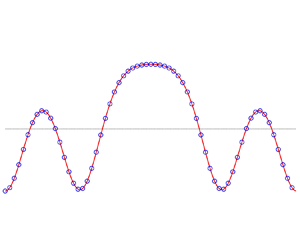
Figure 1. Recovery of a nonlinear capillary–gravity wave with period $L = 6{\rm \pi} d$, Froude number square $B/(gd)=1.01568$ and Bond number $\tau /(gd^2)=1/3$. (a) Bottom pressure treated as a ‘measurement’ for the recovery procedure. (b,c) Respectively, recovered surface pressure and profile (blue circles) vs the exact solution (red line).

Figure 2. Same panels as figure 1 for the period $L/d=2{\rm \pi}$, the Froude number square $B/(gd)=2.28113$ and the Bond number $\tau /(gd^2)=2$.

These recoveries were obtained assuming no a priori knowledge of the physical nature of the surface pressure, but assuming that the total wave height has been measured in addition to the bottom pressure. If instead of the total wave height we consider, say, the mean horizontal velocity at the bottom, we were also able to recover both the free surface and surface pressure, with similar accuracy for $\eta$ (${\sim }10^{-8}$) and $B$ (${\sim }10^{-10}$).

With knowledge of the physical nature of the surface pressure, we were also able to recover the free surface without extra measurements besides the bottom pressure. This is obtained by minimising an error between the reconstructed and theoretical surface pressure as explained in § 3.4. Our preliminary numerical investigations seem to indicate that the choice of the error to minimise plays a role in the speed and accuracy of the recovery procedure. A thorough numerical investigation of this optimisation problem is way beyond the scope of this short paper, of which the purpose is a proof of concept to attest the possibility to recover both the free surface and the surface pressure.

6. Discussion

We derived expressions for free-surface and surface-pressure recoveries, assuming the physical effects at the free surface or considering additional measurements. Then, we illustrated the practical procedure with a fast and simple numerical algorithm. The method proposed here is more general in substance than previous studies by Clamond (2013), Clamond & Constantin (2013), Clamond & Henry (2020), and can be generalised to incorporate linear shear currents along the lines of Clamond et al. (2023). This approach can further be extended to accommodate overhanging waves (existing in the presence of capillary and/or vorticity) as recently shown by Labarbe & Clamond (2023).

So far, we have considered recovery procedures from bottom-pressure measurements, but similar relations could be derived considering the pressure at another depth, as well as other measured physical quantities. Further extensions to configurations with non-permanent wave motions or arbitrary vorticity, for example, are also of great interest, but present technical challenges beyond the scope of this current work.

In this short paper, we demonstrated the possibility to recover the free surface with an arbitrary surface pressure, and we briefly illustrated the procedure with a few examples. We did not address the (difficult) question of uniqueness of the free surface from a given bottom pressure. Indeed, for instance, capillary–gravity waves are not unique for identical physical parameters (Buffoni, Groves & Toland 1996; Clamond, Dutykh & Durán 2015). This example indicates, although the recovery from bottom measurements is a slightly different problem, that the question of uniqueness is important, both theoretically and practically, and it should be the subject of future investigations.