Impact of laterally mobile surface charge on diffusiophoresis of hydrophobic rigid colloids

Abstract

The diffusiophoresis of charged hydrophobic nanoparticles (NPs) governed by an imposed ionic concentration gradient is analysed. The main objective is to elucidate the impact of the laterally mobile adsorbed surface ions at the interface on the propulsion of the hydrophobic NPs in diffusiophoresis. In addition, the dielectric polarization due to the difference in dielectric constant between the NPs and the suspension medium is also considered. The mobile surface ions create a friction as well as an electric force at the hydrophobic surface, which leads to a modification of the slip velocity condition and the slip length. We obtain an exact numerical solution of the governing electrokinetic equations in their full form by adopting a control volume formulation. The numerical model is supplemented by analytical solutions derived based on the Debye–Hückel linearization. We find that the lateral mobility of the surface ions obstruct the coions to diffuse from the higher concentration side to the lower concentration side, which results in a repulsive force to the particle leading to the occurrence of a negative mobility. Based on the numerical results and analytical solutions, we have shown that for a fully mobile surface charge, the diffusiophoresis of a hydrophobic NP is identical to the diffusiophoresis of a liquid droplet whose viscosity is related to the slip length of the hydrophobic particle. We establish that the dielectric polarization enhances the velocity of a hydrophobic particle, which has potential applications in the practical context.

1. Introduction

Diffusiophoresis is an important electrokinetic phenomenon that describes the transport of colloidal entities in a solution of electrolytes or non-electrolytes under the influence of an imposed concentration gradient. Diffusiophoresis has drawn wide interest due to its relevance in numerous processes such as colloid separation enabled by ${\rm CO}_2$-induced diffusiophoresis (Shimokusu et al. 2019), colloid stratification during drying (Sear & Warren 2017), oil recovery (Yang, Shin & Stone 2018), detection and healing of bone fracture (Yadav et al. 2013), separation and purification (Meisen et al. 1971; Carstens & Martin 1982), surface adhesion and coating (Korotkova & Deryagin 1991), DNA sequencing (Shin et al. 2017) as well as to drive catalytic nano- and micromotors (Sen et al. 2009). Diffusiophoresis can transport colloids in a dead-end pore and produce no Joule heating due to net zero current through the suspension medium. These are more suitable in translocation and characterizing living cells as compared with electrophoresis or pressure-driven flows (Lee 2019).

The diffusiophoresis induced by an imposed concentration gradient in an electrolyte is more complicated than that of the non-electrolyte medium. The charged colloid induces an electric double layer (EDL), which deforms under the influence of the applied concentration field and, in turn, creates the double layer polarization (DLP). Diffusiophoresis is a combination of two distinct electrokinetic effects, namely, chemiphoresis and induced electrophoresis (Prieve et al. 1984; Prieve & Roman 1987). The former effect arises due to the DLP, which, in turn, leads to an induced local electric field. The electrophoresis part is solely induced by the diffusion field arising due to the difference in the diffusion coefficient of ionic species present in the electrolyte. In general, the electrophoresis and chemiphoresis effects cannot be separated as the diffusion field influences the DLP as well as the DLP effect modifies the local electric field. Based on a thin EDL consideration, Prieve et al. (1984) has provided a mathematical expression for the electrophoresis and chemiphoresis parts valid for a lower range of surface charge density.

Over the years, several studies have been made on diffusiophoresis under a finite Debye layer consideration (Hsu, Hsu & Chen 2009; Fang & Lee 2015; Lee 2019; Ohshima 2022). Based on theoretical analysis (Hsu et al. 2009; Fang & Lee 2015) the mobility reversal at a higher $\zeta$-potential due to the occurrence of the type-II double layer polarization (DLP-II) is demonstrated. At a higher $\zeta$-potential, the stronger electrostatic force created by the surface ions prevents the diffusion of coions across the Debye layer. This leads to a larger accumulation of coions at the higher concentration side (DLP-II), creating a stronger repulsive force to the particle and pushing the particle towards the lower concentration side, resulting in a mobility reversal. In droplet diffusiophoresis, the mobility reversal may happen at a lower surface potential due to the DLP-II effect caused by a locally induced electric field (Tsai et al. 2022). Several experimental studies (Nery-Azevedo, Banerjee & Squires 2017; Shimokusu et al. 2019; Shin 2020; Wilson et al. 2020) corroborate the theoretical findings of the diffusiophoresis of colloidal entities.

Most of the existing studies on the electrokinetics over hydrophobic surfaces considered the slip velocity condition as being independent of the surface charge. The hydrophobic behaviour of the solid substrate is characterized by the smaller solid–fluid cohesivity parameter appearing in the Leonard-Jones potential, which determines the interaction of the fluid and solid molecules. In addition, the surface ions interact with the solvent ions by the Coulomb potential. Thus, the friction at the hydrophobic interface is influenced by the electric force created by the surface charge. The slip length, which is the ratio of the liquid viscosity to the interfacial friction coefficient, must depend on the surface charge. Based on the stress balance condition incorporating the electric force created by the surface charge, Joly et al. (2004) proposed a surface charge-dependent slip length. The molecular dynamics simulation of Xie et al. (2020) established the dependence of slip length on the surface charge density. Several experimental studies (Pan & Bhushan 2013; Jing & Bhushan 2015) have established that the slip length diminishes with the higher accumulation of surface charge. The experimental and theoretical analysis of Kobayashi (2020) on the electrophoresis of hydrophobic polystyrene nanoparticles concludes that the slip length is larger for a lower surface charge density.

The slip velocity effects on a hydrophobic solid surface can be interpreted through the ‘gas cushion model’ (Vinogradova 1995), which combines a thin layer of decreased viscosity with mobile surface ions located at the interface and immobile ions are fixed at a solid surface (Vinogradova, Silkina & Asmolov 2023). Maduar et al. (2015) demonstrated that in response to an electric field, the adsorbed charges on a hydrophobic surface are laterally mobile with respect to the fluid. Physisorption of the surface charge on the slippery hydrophobic surface is demonstrated in experimental studies (Dammer & Lohse 2006). This has been corroborated by ab initio simulations (Sendner et al. 2009). Based on the molecular dynamics simulations on electrokinetic transport through hydrophobic carbon and hexagonal boron nitride (hBN) nanotubes, Mangaud et al. (2022) established that the experimental data for the surface state can be deduced correctly by considering the mobility of the physisorbed surface charge. The laterally mobile surface ions can arise due to the adsorption of basic and/ or acidic surfactants (Mouterde & Bocquet 2018). The wetting properties of naturally hydrophilic ${\rm SiO}_2$ nanoparticles are manipulated using ionic surfactants (Liang et al. 2019). The experimental study (Galarza-Acosta et al. 2023) reveals a weak adsorption of surfactant molecules onto the ${\rm SiO}_2$ nanoparticles. The experimental and theoretical study by Uematsu, Bonthuis & Netz (2020) demonstrates that the sizable amount of $\zeta$-potential on a hydrophobic surface, as determined experimentally, may arise due to the adsorption of surface active agents present in the suspension medium.

The laterally mobile surface ions (physisorbed ions) create a friction force as well as an electric force at the hydrophobic interface. Several authors (Mouterde & Bocquet 2018; Liang et al. 2019; Mouterde et al. 2019; Xie et al. 2020; Liu, Xing & Pi 2022) studied the impact of the mobile surface charge in the context of electrokinetics over charged slippery flat surfaces. It may be noted that Maduar et al. (2015) and the subsequent study by Vinogradova, Silkina & Asmolov (2022) neglected the electric force in the fluid friction at the charged hydrophobic interface and thus the slip length is independent of the surface charge density in those studies. However, electrokinetics around a curved surface becomes complicated due to the development of a non-uniform induced tangential electric field. This unknown induced electric field influences the slip condition at the hydrophobic curved surface. The laterally mobile surface ions along the surface of a hydrophobic colloid create hydrodynamic friction and a tangential electric force, which can modify the local electric field as well as create resistance to the propulsion of hydrophobic nanoparticles (NPs). Thus, the electrokinetics is expected to have a strong influence due to the presence of the mobile surface charge.

Despite the relevance of the charged surface wettability condition in several practical contexts (Van Loosdrecht et al. 1987; Kobayashi 2020), studies on its influence on diffusiophoresis are rather limited. Recently, Majhi & Bhattacharyya (2022) imposed a Navier-slip condition to analyse the influence of surface wettability on diffusiophoresis. In this paper, we consider the diffusiophoresis of a polarizable hydrophobic charged particle. The adsorbed surface charge on the hydrophobic colloid is considered to be laterally mobile, which leads to a modification of the slip velocity condition involving both hydrodynamic friction and electric force. The hydrophobic colloids such as DNA or protein can have a dielectric permittivity different from the electrolyte medium (Loeb 1924; Shukla & Mikkola 2020). In such cases, the colloid can polarize and create an induced surface charge. Due to the anti-symmetric distribution of the induced surface charge, the electrophoresis part may remain invariant. It also does not alter the tangential stress balance condition at the interface. However, the induced charge can modify the DLP and, hence, affect the diffusiophoresis. A theoretical analysis on the diffusiophoresis of such a type of colloids has not been addressed in the literature.

In the present study, the mathematical model is based on the conservation principle. A modified interfacial slip condition is developed through a balance of hydrodynamic and electric stress created by the weakly adsorbed laterally mobile surface ions. The electric force on the surface charge enables the effective slip length to vary with the surface charge density. Thus, the slip boundary condition is coupled with the induced electric field, which is governed by the local distribution of ions. We develop a finite volume based numerical scheme to solve the governing equations in their full form. In addition, we adopt a regular perturbation analysis to linearize the governing equation and an explicit analytical solution for diffusiophoretic mobility is developed under the Debye–Hückel (D–H) limit. Thus, the present model applicable for polarizable and hydrophobic charged particles with mobile surface charge will pave the way for the experimentalist to measure the intrinsic parameters associated with the colloid particle based on the diffusiophoresis correctly.

Several authors (Uematsu et al. 2020, and the references therein) established that the mechanisms for the electrification of hydrophobic solid surfaces are similar to those of bubble or droplet surfaces. In this study, based on the numerical solution as well as the analytical expression under the D–H approximation, we attempt to show an equivalence between the diffusiophoresis of a hydrophobic colloid with fully mobile surface charge and a charged droplet.

2. Mathematical model

We consider the diffusiophoresis of a hydrophobic colloidal particle of radius $a$ in an electrolyte solution of viscosity $\eta$ under an externally imposed concentration gradient $\boldsymbol {\nabla } n_{\infty }$, which enables the particle to translate with a uniform speed $U_{D}$ with respect to the suspension medium. The dielectric permittivity of the particle and aqueous medium are, in general, different and are denoted by $\epsilon _{p}$ and $\epsilon _{e}$, respectively. We consider the particle surface to be hydrophobic, which acquires a uniform surface charge density $\sigma$ as a result of the weak physisorption of a specific ionic species at the surface. The mobile nature of such ions significantly modifies the hydrodynamic slip condition (Maduar et al. 2015; Mouterde & Bocquet 2018; Vinogradova et al. 2022). A spherical polar coordinate system ($r,\theta,\psi$) is considered with its origin (figure 1) held fixed at the centre of the particle, and the $z$-axis ($\theta =0$) is taken along the imposed concentration gradient $\boldsymbol {\nabla } n_{\infty }$. With respect to this stationary coordinate frame fixed at the particle centre, the far-field fluid is considered to approach with a velocity $-U_{D}$ towards the particle.

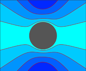
Figure 1. A schematic illustration of the diffusiophoresis of a hydrophobic polarizable particle and the spherical coordinate system.

The scaled electric potential ($\phi$), scaled by the thermal potential $\phi _{0}$, within the electrolyte is governed by the Poisson equation,

(2.1)\begin{equation} \nabla ^{2}\phi={-}\frac{(\kappa a)^{2}}{2}\rho_e,\quad r>1, \end{equation}

where $\rho _e=\sum _{i=1}^{N}z_{i}n_{i}$ is the scaled space charge density. Here, $z_{i}$ and $n_{i}$ are the valence and the concentration of the $i{\text {th}}$ ionic species, respectively. The ionic concentration is scaled by the bulk ionic strength $I=(1/2)\sum _{i=1}^{N}{z^{2}_{i}n^{\infty }_{i}}$, where $n^{\infty }_{i}$ is the bulk concentration of the $i{\text {th}}$ ionic species and can be measured from $n_{\infty }$, which is the ionic concentration at $r=0$ in the absence of the particle.

As there is no free charge inside the particle, the electric potential inside the particle ($\bar {\phi }$) is governed by the Laplace equation, i.e.

(2.2)\begin{equation} \nabla ^{2}\bar{\phi}=0,\quad r<1. \end{equation}

The boundary conditions of the electric potential along the particle surface are

(2.3a,b)\begin{equation} \frac{\partial \phi}{\partial r}-\epsilon_{r}\frac{\partial \bar{\phi}}{\partial r}={-}\sigma, \quad \bar{\phi}=\phi. \end{equation}

Here, the first condition corresponds to the jump discontinuity of the dielectric displacement vector and the second condition is due to the continuity of the potential. Additionally, $\epsilon _{r}~(=\epsilon _{p}/\epsilon _{e}$) is the particle to electrolyte permittivity ratio and $\sigma$ is scaled surface charge density scaled by $\epsilon _{e}\phi _{0}/a$.

The Nernst–Planck equation governing the spatial distribution of the $i\text {th}$ ionic species is

(2.4)\begin{equation} \frac{\partial n_i}{\partial t} +\boldsymbol{u}\boldsymbol{\cdot}\boldsymbol{\nabla} n_i=\frac{1}{Pe_{i}}\boldsymbol{\nabla}\boldsymbol{\cdot}(n_{i} \boldsymbol{\nabla} \mu_{i}), \end{equation}

where $\mu _{i}$ is the dimensionless electrochemical potential of the $i\text {th}$ ionic species, scaled by $k_{B}T$, and is defined as

(2.5)\begin{equation} \mu_{i}=\mu^{0}_{i}+z_{i}\phi+\ln{n_{i}}. \end{equation}

Here, $\boldsymbol {u}=(v,u)$ is the velocity vector with $v$ the radial and $u$ the cross-radial velocity components, scaled by $U_{0}=\epsilon _{e}\phi ^{2}_{0}/\eta a$, and $t$ is the dimensionless time which is scaled by $a/U_{0}$. The Péclet number $Pe_{i}=\epsilon _{e}\phi ^{2}_{0}/\eta D_{i}$ provides the importance of advective to diffusive transport of ions, where $D_i$ is the diffusion coefficient of the $i\text {th}$ ionic species. The no normal flux of ions at the particle surface leads to the boundary condition at $r=1$ as

(2.6)\begin{equation} \boldsymbol{\nabla}{\mu_{i}}\boldsymbol{\cdot} \boldsymbol{e}_{r}=0, \end{equation}

where $\boldsymbol {e}_{r}$ is the unit normal vector pointing outwards at the particle surface.

The equation of incompressible Newtonian fluid describing the motion of ionized fluid can be expressed in scaled form as

(2.7)$$\begin{gather} Re\frac{\partial \boldsymbol{u}}{\partial t} + Re(\boldsymbol{u}\boldsymbol{\cdot}\boldsymbol{\nabla})\boldsymbol{u}- \nabla^{2}\boldsymbol{u} +\boldsymbol{\nabla} p + \frac{(\kappa a)^{2}}{2} \rho_e \boldsymbol{\nabla}\phi =0, \end{gather}$$

(2.8)$$\begin{gather}\boldsymbol{\nabla}\boldsymbol{\cdot}\boldsymbol{u}=0, \end{gather}$$

where pressure $p$ is the scaled pressure by $\epsilon _{e}\phi ^{2}_{0}/a^{2}$ and other scales for other variables are defined earlier. The Reynolds number associated with the electrokinetic motion of colloidal entities is generally small and the flow field is also axisymmetric in nature. We assume the $z$-axis as the axis of symmetry.

We consider lateral mobility of the adsorbed surface charge on the hydrophobic surface. The interfacial friction modifies by the electric force created by the surface charge, which leads to the slip length, the ratio between the liquid viscosity to the interfacial friction, at the hydrophobic surface as (Xie et al. 2020)

(2.9)\begin{equation} \lambda_{eff}=\frac{\lambda}{1-6{\rm \pi}(1-\chi_{s})(\tau\epsilon_{e}\phi_{0}/e)\lambda\sigma}, \end{equation}

where $\lambda$ is the slip length corresponding to the uncharged surface (bare slip length) and $\tau$ is the effective hydrodynamic radius of the physisorbed hydroxide ions. Here, $\chi _{s}=\omega _{s}/(\omega _{s}+\omega _{w})$ is a scaled parameter which can be related to the mobility of the surface ions, where $\omega _{s}$ and $\omega _{w}$ are the friction coefficients of the mobile surface ion with water and wall, respectively (Mouterde & Bocquet 2018; Mouterde et al. 2019). Based on the Stokes drag on the hydrated ion of size $\tau _h$, the friction coefficient $\omega _{s}$ can be obtained as $\omega _{s}=3{\rm \pi} \tau _{h}\eta$ (Mangaud et al. 2022), which has the dimension ${\rm kg}\ {\rm s}^{-1}$. In the present formulation, $\omega _{w}$ is appearing through the scaled parameter $\chi _{s}$, which can be determined through the electrophoretic mobility of the physisorbed ions, defined as $1/(\omega _{s}+\omega _{w})$. Several theoretical analyses (Mouterde & Bocquet 2018; Liu et al. 2022) on the electroosmotic flow involving the physisorbed surface ions determined $\chi _{s}$ by considering the experimental data for the electrophoretic mobility of physisorbed ions, as reported by Mouterde et al. (2019) and Mangaud et al. (2022). For a rigid hydrophilic wall in which the ion–wall friction $\omega _{w}\to \infty$, then $\chi _{s}=0$, i.e. ions are immobile on the surface. As the surface ions are considered to have lateral mobility, the balance of interfacial stress leads to the modified slip boundary condition as (Majhi, Bhattacharyya & Gopmandal 2024)

(2.10)\begin{equation} u\boldsymbol{e}_{\theta}=\lambda_{eff}\left\{\left(\boldsymbol{\sigma^{H}}+\chi_{s}\left(\boldsymbol{\sigma^{E}}-\boldsymbol{\bar{\sigma}^{\bar{E}}}\right)\right) \boldsymbol{\cdot}\boldsymbol{e}_{r}-\left[\left(\left(\boldsymbol{\sigma^{H}}+\chi_{s}\left(\boldsymbol{\sigma^{E}}-\boldsymbol{\bar{\sigma}^{\bar{E}}}\right)\right) \boldsymbol{\cdot}\boldsymbol{e}_{r}\right)\boldsymbol{\cdot}\boldsymbol{e}_{r}\right]\boldsymbol{e}_{r}\right\}, \end{equation}

where $\boldsymbol {e}_{\theta}$ is the unit tangential vector at the particle surface, $\boldsymbol {\sigma ^{H}}$ denotes the hydrodynamic stress tensor, and the Maxwell stress tensors outside and within the particle are respectively $\boldsymbol {\sigma ^{E}}$ and $\boldsymbol {\bar {\sigma }^{\bar {E}}}$ (Yang et al. 2018). Using (2.3a,b), the above boundary condition for the tangential velocity on the slippery impermeable hydrophobic surface for the axisymmetric problem can be simplified to

(2.11)\begin{equation} u=\lambda_{eff}\left[ r\frac{\partial}{\partial r}\left(\frac{u}{r}\right)-\chi_{s}\sigma\left(\frac{1}{r}\frac{\partial \phi}{\partial \theta}\right)\right]\quad \text{and}\quad v=0\quad \text{at}\ r=1. \end{equation}

For the case of immobile surface charge $\chi _{s}=0$, the friction force created by the electromigration of surface ions becomes zero. The second condition $v=0$ on the surface arises due to the fluid impermeability along the surface of the rigid particle. Note that for a hydrophilic surface, $\lambda =0$, which yields $\lambda _{eff}=0$ and thus, the tangential velocity reduces to zero.

The boundary conditions along the far-field $(r\gg 1)$ in a reference frame fixed at the particle centre are as follows:

(2.12a–c)\begin{equation} \boldsymbol{u}={-}U_D \boldsymbol{e_z}, \quad n_{i}=\frac{n^{\infty}_{i}}{I}(1+\alpha r \cos\theta),\quad\phi={-}\beta\alpha r \cos\theta, \end{equation}

where $U_D$ is the diffusiophoretic velocity, which is unknown a priori and the primary concern is to calculate $U_{D}$. The diffusiophoretic mobility, denoted as $\mu _{D}$, is the diffusiophoretic velocity per unit imposed concentration gradient $\alpha$. Here, ${\alpha ={|\boldsymbol {\nabla }^{*}{n_{\infty }}|a}/{n_{\infty }}}$ is the scaled concentration gradient imposed externally. The term $\beta ={\sum _{i}{D_{i}z_{i}n^{\infty }_{i}}}/{\sum _{i}{D_{i}z^{2}_{i}n^{\infty }_{i}}}$ is the parameter measures the diffusion potential.

At steady state, the unknown diffusiophoretic velocity $U_{D}$ is determined through the balance of electric and drag forces as experienced by the particle. The steady diffusiophoresis of a spherical particle can be considered to be axisymmetric, implying that the azimuthal dependence of the variables can be neglected. Due to this axisymmetry consideration, the force balance only along the $z$-direction can be considered. The electrostatic ($F_E$) and hydrodynamic ($F_D$) forces along the flow direction can be calculated by integrating over the particle surface the Maxwell stress tensor $\boldsymbol {\sigma ^E}$ and hydrodynamic stress tensor $\boldsymbol {\sigma ^H}$, respectively (Majhi & Bhattacharyya 2022). The diffusiophoretic velocity $U_{D}$ and, hence, mobility $\mu _{D}$ is determined by solving the force balance condition $F_E+F_D=0$.

We adopt a numerical procedure to solve the governing electrokinetic equations exactly. In the numerical method, $U_{D}$ is determined iteratively by solving the force balance condition. Based on an approximate $U_{D}$, the governing nonlinear electrokinetic equations are solved in a coupled manner. The diffusiophoresis considered here is a steady process. However, for numerical simulation, the diffusiophoresis is considered to start impulsively from the equilibrium state, which approaches the steady state after a transient phase. A forwards time marching procedure is adopted to solve the governing unsteady equations, which is continued until the time-independent solution is achieved after a transient phase. We adopt a control volume approach with a higher-order upwind discretization for the convection and electromigration terms. A detailed discussion on the numerical method as adopted here is provided elsewhere (Majhi & Bhattacharyya 2022,  2023a). Through this numerical solution, the forces acting on the particle are determined and, subsequently, the solution for $U_{D}$ is updated. The procedure is continued until the force balance condition, within a tolerance limit, is satisfied.

In addition to the exact numerical solution (ENS), we make a theoretical analysis on diffusiophoresis under a weak applied concentration field along with linearized approximation. In this case, we drop the unsteady terms in the governing equations and neglect the convective terms in the momentum equation (2.7). The reduced set of equations considered for the theoretical analysis is provided in Appendix A. The explicit form of the diffusiophoretic velocity is obtained for the low charge limit for which the D–H approximation holds. Below, we provide an outline of the theoretical analysis and derivation of analytical expression for the mobility.

3. Linearized solution under a weak concentration gradient

We adopt a first-order perturbation analysis by considering the imposed concentration gradient scaled by the bulk concentration divided by particle radius, i.e. $\alpha$ as the perturbation parameter. When a concentration difference at the two ends of the domain $n_{\infty,R}-n_{\infty,L}$ is imposed, then $\alpha ={(n_{\infty,R}-n_{\infty,L})a}/[{R(n_{\infty,R}+n_{\infty,L})}]$, where $R$ is the radius of the outer boundary. In general, the domain $R\gg a$, which implies $\alpha \ll 1$. Under this small $\alpha$, all the electrokinetic variables appearing in the above governing equations are considered to be slightly perturbed from their equilibrium condition. The equilibrium condition implies that the gradient of the electrochemical potential is zero and there is no relative motion of fluid and the particle. Based on this perturbation, we can derive the expression for the diffusiophoretic mobility as

(3.1)\begin{equation} \mu_{D}=\frac{1}{9}{\int_{1}^{\infty}\left[\frac{1}{1+2\lambda_{eff}}-{3r^2}+2\frac{(1+3\lambda_{eff})}{(1+2\lambda_{eff})}r^3\right] G(r)\,{\rm d}r}-\frac{2\chi_{s}\lambda_{eff}\sigma}{3(1+2\lambda_{eff})}Y(1). \end{equation}

A detailed derivation of (3.1) based on the linear perturbation analysis is provided in Appendix A. The functions $G(r)$ and $Y(1)$ are obtained by solving a set of boundary value problems, as outlined in Appendix A. We show later that the mobility based on this expression (3.1) matches with the ENS of the governing equations. This simplified model for the mobility (3.1) requires a numerical solution of the set of linear boundary value problems (A4) as provided in Appendix A. Thus, the simplified model is significantly more cost effective as compared with the exact numerical solution, which requires numerical solutions of coupled set of nonlinear partial differential equations. This expression is further simplified by adopting the D–H approximation valid for the range of surface charge density so as to have the surface potential less the thermal potential, i.e. $|\zeta |<1$.

Based on the D–H approximation, the closed form analytical solution for the diffusiophoretic mobility of a hydrophobic particle suspended in a monovalent symmetric electrolyte with distinct diffusion coefficient can be derived as

(3.2)\begin{align} \mu_{D}&= \left[\frac{\sigma}{\kappa a+1}\varTheta_{1}(\kappa a)-\frac{\chi_{s}\lambda_{eff}\sigma K_{1}}{(\epsilon_{r}+K_{1})(1+2\lambda_{eff})}\right]\beta\nonumber\\ &\quad +\left(\frac{\sigma}{\kappa a+1}\right)^{2}\left[\frac{1}{8}\varTheta_{2}(\kappa a)-\frac{2\chi_{s}\lambda_{eff}}{3(\epsilon_{r}+K_{1})(1+2\lambda_{eff})} \right.\nonumber\\ & \quad \times\left. \left\{\frac{21}{4}-\frac{3}{4}\kappa a+\frac{3}{4}(\kappa a)^{2}-3{\rm e}^{\kappa a}E_{5}(\kappa a)+15{\rm e}^{\kappa a}E_{6}(\kappa a)-45{\rm e}^{\kappa a}E_{7}(\kappa a)\right\}\right], \end{align}

where $K_{1}=(1+\kappa a)+(1+\kappa a)^{-1}$, and the functions $\varTheta _{1}(\kappa a)$ and $\varTheta _{2}(\kappa a)$ are respectively given by

(3.3a)\begin{align} \varTheta_{1}(\kappa a)&=\frac{\lambda_{eff}}{1+2\lambda_{eff}}\kappa a+\frac{1+\lambda_{eff}}{1+2 \lambda_{eff}}+2{\rm e}^{\kappa a}E_{5}(\kappa a)-\frac{5}{1+2\lambda_{eff}}{\rm e}^{\kappa a}E_{7}(\kappa a), \end{align}

(3.3b)\begin{align} \varTheta_{2}(\kappa a)&= \frac{2\lambda_{eff}}{1+2\lambda_{eff}}\kappa a+\frac{1}{1+2 \lambda_{eff}}-\frac{8}{3}{\rm e}^{\kappa a}E_{3}(\kappa a)+8{\rm e}^{\kappa a}E_{4}(\kappa a)\nonumber\\ &\quad +\frac{8}{3}\frac{1}{1+2\lambda_{eff}}{\rm e}^{\kappa a}E_{5}(\kappa a)-8\varTheta_{1}(\kappa a) {\rm e}^{\kappa a}E_{5}(\kappa a)-\frac{40}{3}\frac{1}{1+2\lambda_{eff}}{\rm e}^{\kappa a}E_{6}(\kappa a)\nonumber\\ &\quad +\frac{10}{3}{\rm e}^{2\kappa a}E_{6}(2\kappa a)+\frac{7}{3}\frac{1}{1+2\lambda_{eff}}{\rm e}^{2\kappa a}E_{8}(2\kappa a). \end{align}

The details derivation of the above expression is provided in Appendix B. Equation (3.2) is one of the key findings of the present study. It is useful for experimentalists for the correct evaluation of intrinsic hydrodynamic and electrostatic properties of charged colloids based on the diffusiophoresis. We can separate the electrophoresis and chemiphoresis parts in the mobility expression (3.2). The terms multiplied by $\beta$ in (3.2) correspond to the electrophoretic contribution, denoted by $\mu _{E}$, and the remaining terms independent $\beta$ correspond to the chemiphoretic contribution, which is denoted by $\mu _{C}$, i.e. $\mu _{D}=\mu _{E}+\mu _{C}$, where

(3.4a)\begin{align} \mu_{E}&=\left[\frac{\sigma}{\kappa a+1}\varTheta_{1}(\kappa a)-\frac{\chi_{s}\lambda_{eff}\sigma K_{1}}{(\epsilon_{r}+K_{1})(1+2\lambda_{eff})}\right]\beta, \end{align}

(3.4b)\begin{align} \mu_{C}&= \left(\frac{\sigma}{\kappa a+1}\right)^{2}\left[\frac{1}{8}\varTheta_{2}(\kappa a)-\frac{2\chi_{s}\lambda_{eff}}{3(\epsilon_{r}+K_{1})(1+2\lambda_{eff})}\right.\nonumber\\ & \quad\times\left. \left\{\frac{21}{4}-\frac{3}{4}\kappa a+\frac{3}{4}(\kappa a)^{2}-3{\rm e}^{\kappa a}E_{5}(\kappa a)+15{\rm e}^{\kappa a}E_{6}(\kappa a)-45{\rm e}^{\kappa a}E_{7}(\kappa a)\right\}\right]. \end{align}

The mobility expression (3.2) based on the linear-order analysis under the D–H approximation shows that the dielectric polarization has no impact on the mobility when immobile surface charge is considered. A similar conclusion has been made by several authors (O'Brien & White 1978; Bhattacharyya & De 2015) in the context of electrophoresis. However, the dielectric polarization can have an impact when the surface charge becomes mobile, which can be captured even through the first-order analysis.

3.1. Mobility expression for $0\leqslant \chi _{s}<1$

In this subsection, we consider various limiting situations and provide closed form analytical results for diffusiophoretic mobility. For the case of a perfectly dielectric particle ($\epsilon _{r}\to 0$), the expression (3.2) reduces to

(3.5)\begin{align} \mu_{D}&= \left[\frac{\sigma}{\kappa a+1}\varTheta_{1}(\kappa a)-\frac{\chi_{s}\lambda_{eff}\sigma}{(1+2\lambda_{eff})}\right]\beta\nonumber\\ &\quad +\left(\frac{\sigma}{\kappa a+1}\right)^{2}\left[\frac{1}{8}\varTheta_{2}(\kappa a)-\frac{2\chi_{s}\lambda_{eff}(\kappa a+1)}{3(1+2\lambda_{eff})((\kappa a+1)^{2}+1)} \right.\nonumber\\ & \quad \times\left. \left\{\frac{21}{4}-\frac{3}{4}\kappa a+\frac{3}{4}(\kappa a)^{2}-3{\rm e}^{\kappa a}E_{5}(\kappa a)+15{\rm e}^{\kappa a}E_{6}(\kappa a)-45{\rm e}^{\kappa a}E_{7}(\kappa a)\right\}\right]. \end{align}

It is obvious that the electrophoresis part attenuates as the velocity of the surface ions, i.e. $\chi _{s}$, is increased. For a perfectly conducting particle ($\epsilon _{r}\to \infty$), the mobility expression (3.2) reduces to the limiting form as

(3.6)\begin{equation} \mu_{D}=\frac{\sigma}{\kappa a+1}\varTheta_{1}(\kappa a)\beta+\frac{1}{8}\left(\frac{\sigma}{\kappa a+1}\right)^{2}\varTheta_{2}(\kappa a). \end{equation}

Under the Hückel limit (i.e. $\kappa a\to 0$), the mobility expression (3.2) reduces to the following simple form:

(3.7)\begin{equation} \mu_D=\frac{2}{3}\sigma\left[\frac{1+3\lambda_{eff}}{1+2\lambda_{eff}}-\frac{3\chi_{s}\lambda_{eff}}{(\epsilon_{r}+2)(1+2\lambda_{eff})}\right]\beta. \end{equation}

This implies that in the Hückel limit, there is no chemiphoresis contribution in particle mobility, i.e. the mobility is generated by the corresponding electrophoresis part only. Further, for a dielectric particle ($\epsilon _{r}\to 0$), the corresponding mobility expression (3.7) reduces to

(3.8)\begin{equation} \mu_D=\frac{2}{3}\sigma\left[\frac{1+3\lambda_{eff}}{1+2\lambda_{eff}}-\frac{3\chi_{s}\lambda_{eff}}{2(1+2\lambda_{eff})}\right]\beta \end{equation}

and in the case of perfectly conducting particle ($\epsilon _r \to \infty$), the above expression (3.7) reduces to

(3.9)\begin{equation} \mu_D=\frac{2}{3}\sigma\left[\frac{1+3\lambda_{eff}}{1+2\lambda_{eff}}\right]\beta. \end{equation}

It is clear by comparing (3.8) and (3.9) that the mobility for a hydrophobic particle is enhanced for the conducting particle as compared with the non-conducting case. Setting $\lambda =0$, we can deduce the Hückel limit $\mu _D=(2/3)\beta \sigma$ applicable for a hydrophilic particle.

We now consider the Smoluchowski limit for a thin EDL, i.e. $\kappa a \gg 1$. The surface charge density for a low-charged particle is related to $\zeta$-potential by the relation $\sigma =\kappa a \zeta$. Based on the order of magnitude analysis, the mobility expression (3.2) can be reduced to

(3.10)\begin{align} \mu_{D}&=\zeta\left[\frac{\lambda_{eff}\kappa a+1}{1+2\lambda_{eff}}-\frac{\chi_{s}\lambda_{eff}(\kappa a)^{2}}{(1+2\lambda_{eff})(\epsilon_{r}+\kappa a)}\right]\beta\nonumber\\ &\quad +\frac{\zeta^{2}}{8}\left[\frac{2\lambda_{eff}\kappa a+1}{1+2\lambda_{eff}}-\frac{4\chi_{s}\lambda_{eff}(\kappa a)^{2}}{(1+2\lambda_{eff})(\epsilon_{r}+\kappa a)}\right]. \end{align}

We find from (3.10), which is valid for a thinner Debye length, that the dielectric polarization has no effect on the mobility when the surface charge is immobile, i.e. $\chi _{s}=0$. This supports the existing study by Schnitzer & Yariv (2012), which shows that the dielectric polarization does not alter the leading-order electrokinetics for a thin EDL. It is evident that both the electrophoresis ($\mu _{E}$) and chemiphoresis ($\mu _{C}$) parts augment as the permittivity of the particle is increased, and this augmentation is proportional to $\chi _{s}$. For a perfectly conducting particle $\epsilon _{r}\to \infty$, the chemiphoresis part becomes positive and the dependence on $\chi _{s}$ appears only through the modification of the effective slip length $\lambda _{eff}$. For a perfectly dielectric particle, (3.10) further reduces to

(3.11)\begin{equation} \mu_{D}=\zeta\left[\frac{1+\lambda_{eff}\kappa a}{1+2\lambda_{eff}}-\frac{\chi_{s}\lambda_{eff}\kappa a}{(1+2\lambda_{eff})}\right]\beta+\frac{\zeta^{2}}{8}\left[\frac{1+2\lambda_{eff}\kappa a}{1+2\lambda_{eff}}-\frac{4\chi_{s}\lambda_{eff}\kappa a}{1+2\lambda_{eff}}\right]. \end{equation}

Hence, under the Smoluchowski limit ($\kappa a\gg 1$), the corresponding electrophoretic and chemiphoretic mobility of a perfectly dielectric particle can be expressed as

(3.12a,b)\begin{equation} \mu_{E}=\zeta\left[\frac{1+(1-\chi_{s})\lambda_{eff}\kappa a}{1+2\lambda_{eff}}\right]\beta\quad \text{and}\quad \mu_{C}=\frac{\zeta^{2}}{8}\left[\frac{1+2(1-2\chi_{s})\lambda_{eff}\kappa a}{1+2\lambda_{eff}}\right]. \end{equation}

It is clear from (3.12a,b) that the sign of $\mu _{E}$ is governed by $\beta \sigma$ and for a fixed $\beta$ and $\sigma$, no change of sign in $\mu _{E}$ occurs as $\chi _{s}\leqslant 1$. The magnitude of $\mu _{E}$ reduces as the surface ions become mobile, i.e. with the increase of $\chi _{s}$. However, the chemiphoretic mobility $\mu _{C}$ remains positive for $\chi _{s}\leqslant 0.5$ and it changes its sign from positive to negative for $\chi _{s}>0.5+0.25(\lambda _{eff}\kappa a)^{-1}$ with $\mu _{C}=0$ at the critical $\chi _{s}$ as $0.5+0.25(\lambda _{eff}\kappa a)^{-1}$. This implies that at a thinner Debye length and/ or higher slip length, $\mu _{C}$ becomes negative when $\chi _{s}$ becomes marginally bigger than $0.5$. Thus, the thin layer analysis shows that the mobility of surface ions $\chi _{s}$ attenuates chemiphoretic mobility when $\chi _{s}<0.5+0.25(\lambda _{eff}\kappa a)^{-1}$ and the mobility for $\beta \sigma >0$ can become negative and can enhance with $\chi _{s}$ for $\chi _{s}>0.5+0.25(\lambda _{eff}\kappa a)^{-1}$.

We find that the mobility of a perfectly dielectric hydrophobic particle ($\epsilon _{r}=0$) may change its sign even if $\beta$ and $\sigma ~(\text {or}~\zeta )$ are fixed, and $\mu _{D}$ may become zero at $\chi _{s}={(1+2\kappa a\lambda _{eff})\zeta +8\beta (1+\kappa a\lambda _{eff})}/{4\kappa a\lambda _{eff}(2\beta +\zeta )}$ at a thin EDL, where $\zeta =\sigma /\kappa a$. The knowledge of mobility reversal is extremely important in various biomedical applications specially in drug delivery, in which the propulsion of the nanoparticle along the direction of the imposed concentration gradient is needed. When the slip length is much smaller than the particle radius, i.e. the dimensionless effective slip length $\lambda _{eff}\ll 1$, the mobility expression (3.11) becomes

(3.13)\begin{equation} \mu_{D}=\beta\zeta[{1+(1-\chi_{s})\lambda_{eff}\kappa a}]+\frac{\zeta^{2}}{8}[1+2(1-2\chi_{s})\lambda_{eff}\kappa a]. \end{equation}

It is evident that the effect of slip amplifies as the Debye length becomes thinner and declines as the surface ions become mobile. For the case of immobile surface charge ($\chi _{s}=0$), the mobility becomes

(3.14)\begin{equation} \mu_{D}={\beta\zeta}({1+\lambda_{eff}\kappa a})+\frac{\zeta^{2}}{8}({1+2\lambda_{eff}\kappa a}), \end{equation}

which is identical with the analytical expression as derived by Majhi & Bhattacharyya (2022) for a hydrophobic particle with immobile surface charge ($\chi _{s}=0$) under a low surface potential when $\lambda _{eff}=\lambda$. The expression for the electrophoresis part shows that the $\zeta$-potential is amplified by a factor $(1+\kappa a\lambda _{eff})$, which follows the concluding remark of Khair & Squires (2009) in the context of electrophoresis of a hydrophobic particle under a thin EDL consideration. For a hydrophilic particle, i.e. $\lambda =0$, the mobility expression (3.14) reduces to

(3.15)\begin{equation} \mu_{D}={\beta\zeta}+\frac{\zeta^{2}}{8}, \end{equation}

which is exactly the same expression as derived by Prieve et al. (1984) for a thin Debye layer under the D–H approximation.

3.2. Mobility expression for $\chi _{s}=1$ and resemblance to a viscous droplet

The mobility expression of a hydrophobic rigid colloid with fully mobile surface charge may be derived from (3.2) by setting $\chi _s=1$, i.e.

(3.16)\begin{align} \mu_{D}&= \left[\frac{\sigma}{\kappa a+1}\varTheta_{1}(\kappa a)-\frac{\lambda\sigma K_{1}}{(\epsilon_{r}+K_{1})(1+2\lambda)}\right]\beta\nonumber\\ &\quad +\left(\frac{\sigma}{\kappa a+1}\right)^{2}\left[\frac{1}{8}\varTheta_{2}(\kappa a)-\frac{2\lambda}{3(\epsilon_{r}+K_{1})(1+2\lambda)}\right.\nonumber\\ & \quad\times \left. \left\{\frac{21}{4}-\frac{3}{4}\kappa a+\frac{3}{4}(\kappa a)^{2}-3{\rm e}^{\kappa a}E_{5}(\kappa a)+15{\rm e}^{\kappa a}E_{6}(\kappa a)-45{\rm e}^{\kappa a}E_{7}(\kappa a)\right\}\right]. \end{align}

When $\chi _{s}=1$, the $\lambda _{eff}$ becomes $\lambda$. Several researchers (Gopmandal, Bhattacharyya & Ohshima 2017; Ohshima 2019; Uematsu et al. 2020) have established a similarity in the electrokinetic transport of hydrophobic colloids with liquid droplets. We now attempt to establish such similarity in diffusiophoresis between liquid droplets and hydrophobic colloids. It is evident that the mobility expression (3.16) becomes identical to the expression for the mobility of a droplet of viscosity $\eta _d=\eta /3\lambda$ as derived by Samanta et al. (2023b). Thus, the diffusiophoresis of a hydrophobic colloid with slip length $\lambda$ for a fully mobile adsorbed surface charge is equivalent to that of a dielectric droplet with viscosity ratio of the droplet-to-fluid $\eta _{r}=1/3\lambda$. We have shown later in § 4 that our numerical simulation for the fully mobile surface ions ($\chi _{s}=1$) agrees exactly with the numerical results of Fan et al. (2022) for a liquid droplet with droplet-to-fluid viscosity ratio $\eta _{r}= 1/3\lambda$.

It may be noted that Tsai et al. (2022) derived an expression for the mobility of a droplet under the D–H approximation, which involves integrals that cannot be evaluated analytically. However, the present expression for the mobility (3.16) as derived based on the D–H approximation does not involve any complicated exponential integrals.

Under the Hückel limit $(\kappa a\ll 1)$, the mobility expression (3.16) reduces to

(3.17)\begin{equation} \mu_D=\frac{2}{3}\sigma\left[\frac{1+3\lambda}{1+2\lambda}-\frac{3\lambda}{(\epsilon_{r}+2)(1+2\lambda)}\right]\beta. \end{equation}

It is evident that the second term of the expression (3.17) reduces with the increase of $\epsilon _{r}$, which implies that the mobility increases with the increase of $\epsilon _{r}$. If we further consider $\epsilon _r \to \infty$ (conducting particle), the above expression (3.17) reduces to

(3.18)\begin{equation} \mu_D=\frac{2}{3}\sigma\left[\frac{1+3\lambda}{1+2\lambda}\right]\beta. \end{equation}

It is clear that $|\mu _{D}|$ is higher for the conducting particle than the dielectric particle.

Under the Smoluchowski limit ($\kappa a \gg 1$), the mobility of a hydrophobic particle with fully mobile surface ions is obtained as

(3.19)\begin{align} \mu_{D}=\zeta\left[\frac{\lambda \kappa a+1}{1+2\lambda}-\frac{\lambda(\kappa a)^{2}}{(1+2\lambda)(\epsilon_{r}+\kappa a)}\right]\beta+\frac{\zeta^{2}}{8}\left[\frac{2\lambda\kappa a+1}{1+2\lambda}-\frac{4\lambda(\kappa a)^{2}}{(1+2\lambda)(\epsilon_{r}+\kappa a)}\right], \end{align}

where $\zeta$ is obtained as $\zeta =\sigma /\kappa a$. Hence, under the Smoluchowski limit, the corresponding electrophoretic and chemiphoretic mobility of a polarizable particle can be separated as

(3.20a,b)\begin{equation} \left.\begin{gathered}\mu_{E}=\zeta\left[\frac{\lambda \kappa a+1}{1+2\lambda}-\frac{\lambda(\kappa a)^{2}}{(1+2\lambda)(\epsilon_{r}+\kappa a)}\right]\beta\\ \text{and}\\ \mu_{C}=\frac{\zeta^{2}}{8}\left[\frac{2\lambda\kappa a+1}{1+2\lambda}-\frac{4\lambda(\kappa a)^{2}}{(1+2\lambda)(\epsilon_{r}+\kappa a)}\right] \end{gathered}\right\}. \end{equation}

For a perfectly dielectric particle, the above electrophoretic and chemiphoretic mobility expressions are reduced to

(3.21a,b)\begin{equation} \mu_{E}=\zeta\left[\frac{1}{1+2\lambda}\right]\beta\quad \text{and}\quad \mu_{C}=\frac{\zeta^{2}}{8}\left[\frac{1-2\lambda\kappa a}{1+2\lambda}\right]. \end{equation}

We find that $\mu _{C}$ and $\mu _{E}$ may act concurrently when $\kappa a \lambda >0.5$ even when $\beta \sigma >0$. It is evident that for larger slip length, $\mu _{E}$ becomes small and $\mu _{C}<0$, leading to $\mu _{D}<0$. Again, the ratio of $\mu _{E}$ and $\mu _{C}$ is

(3.22)\begin{equation} \frac{\mu_{E}}{\mu_{C}}=\frac{8\beta}{\zeta}\left[\frac{1}{1-2\kappa a\lambda}\right]. \end{equation}

Since $\kappa a\gg 1$, which implies $\kappa a \lambda \gt \gt 1$ when $\lambda \sim O(1)$, in such a situation, $|\mu _{E}/\mu _{C}|\simeq 4|\beta |/(\lambda |\sigma |)$. Therefore, $|\mu _{C}|>|\mu _{E}|$ under the condition $\lambda >4|\beta |/|\sigma |$. This implies that $\mu _{D}<0$ when $\lambda >4|\beta |/|\sigma |$ even when $\beta \sigma >0$. Again, when $\lambda \gg 1$, i.e. in the superhydrophobic situation, $\mu _{E}\to 0$ and $\mu _{C}$ becomes $-\sigma \zeta /8$, which implies that $\mu _{D}<0$ regardless the values of $\sigma$ and $\beta$.

When the particle becomes perfectly conducting, (3.20a,b) becomes

(3.23a,b)\begin{equation} \mu_{E}=\zeta \left[\frac{\lambda \kappa a+1}{1+2\lambda}\right]\beta\quad \text{and}\quad \mu_{C}=\frac{\zeta^{2}}{8}\left[\frac{2\lambda\kappa a+1}{1+2\lambda}\right]. \end{equation}

It is clear that for a conducting particle, $\mu _{C}$ remains positive and $\mu _{E}$ is positive for $\beta \sigma >0$. Hence, the mobility of a conducting particle remains positive if $\beta \sigma >0$ and can change sign for $\beta \sigma <0$. Furthermore, $\mu _{E}$ and $\mu _{C}$ reduce to $\beta \sigma /2$ and $\sigma \zeta /8$, respectively, in the super-hydrophobic situation $\lambda \gg 1$, which implies that $|\mu _{E}|>|\mu _{C}|$ when $|\zeta |<4|\beta |$. Thus, $|\mu _{E}|$ is dominant for lower $\zeta$-potential; however, $|\mu _{C}|$ dominants when $\zeta$-potential increases to more than four times the diffusion potential when slip length $\lambda \gg 1$.

From expression (3.20a,b), it can be observed that $\mu _{E}$ increases with $\epsilon _{r}$ and reaches its maximum when the particle is conducting ($\epsilon _{r} \to \infty$) and mobility remains positive for $\beta \sigma >0$. However, $\mu _{C}=0$ exactly at $\epsilon _{r}=4\lambda (\kappa a)^{2}/(2\lambda \kappa a+1)-ka$ or at $\epsilon _{r}\simeq \kappa a-\lambda ^{-1}$ if $2\lambda \kappa a>1$, which agrees with the numerical finding of Majhi & Bhattacharyya (2023b) for a charged droplet. Subsequently, $\mu _{C}\leqslant 0$ when $\epsilon _{r}\leqslant \kappa a-\lambda ^{-1}$ and becomes positive when $\epsilon _{r}> \kappa a-\lambda ^{-1}$. Furthermore, when $\mu _{C}> 0$, the magnitude of $\mu _{C}$ enhances as $\epsilon _{r}$ increases, and when $\mu _{C}$ is negative, $|\mu _{C}|$ behaves as a decreasing function of $\epsilon _{r}$. One may note that the mobility $\mu _{D}$ is always positive when $\epsilon _{r}> \kappa a-\lambda ^{-1}$ as $\mu _{E}$ is always positive when $\beta \sigma >0$.

The analytical solution under the D–H approximation for several limiting conditions can be summarized as follows. The mobility expression for a dielectric particle is given in (3.5) and the expression for a conducting particle is given in (3.6). The Hückel limit is given in (3.7), which reduces to the expressions for a dielectric and a conducting particle in (3.8) and (3.9), respectively. The mobility under the Smoluchowski limit can be expressed by (3.10). Under the consideration of the Smoluchowski limit, $\mu _{D}$ for a dielectric particle is given in (3.11), which reduces to (3.13) for a low slip length $\lambda \ll 1$. This can be further reduced to the expression (3.14) for the immobile surface ions ($\chi _{s}=0$) and (3.15) for a hydrophilic particle ($\lambda =0$). For the fully mobile surface charge ($\chi _{s}=1$), $\mu _{D}$ is governed by (3.16) and the corresponding Hückel limit for $\mu _{D}$ is given in (3.17). The Hückel limit for $\mu _{D}$ of a conducting particle is given in (3.18). The Smoluchowski limit for $\mu _{D}$ of a polarizable hydrophobic particle with fully mobile surface charge is given in (3.19). The corresponding expression for mobility for a dielectric and a conducting particle are obtained from (3.21a,b) and (3.23a,b), respectively.

4. Results and discussion

The results are obtained based on the parameter values $\rho =10^{3}\ \textrm {kg}\ \textrm {m}^{-3}$, $\eta =10^{-3}\ \textrm {Pa}\ \textrm {s}$, $\epsilon _{e}=695.39\times 10^{-12}\ \textrm {C}\ (\textrm {V}\ \textrm {m})^{-1}$ and $e=1.602\times 10^{-19}$ at a constant temperature $T=298\ \textrm {K}$. We consider the scaled imposed concentration gradient $\alpha =10^{-3}$, which is close to the value considered in the experimental study by Ebel, Anderson & Prieve (1988). The valency and diffusion coefficient of the electrolytes considered in this study are given in table 1. We begin with a comparison of our numerical algorithm with the existing experimental results and the simplified model, as well as the linearized model for the limiting cases.

Table 1. Values of $z_+$, $z_-$, $D_+$, $D_-$ and $\beta$ for some common electrolytes at $25\,^{\circ }\textrm {C}$.

4.1. Comparison with existing results and present analytical solutions

Figure 2(a) depicts the comparison of our ENS with the experimental results of Ebel et al. (1988) for the diffusiophoretic mobility of a hydrophilic ($\lambda =0$) latex particle for different electrolyte solutions. At each $\kappa a$ for which $\mu _{D}$ is computed, the surface charge density is different and can be found from Ebel et al. (1988). An excellent agreement is found between the experimental results and our computed results. The mobility is positive for KCl as it is governed by the chemiphoresis part only. For LiCl and NaCl, the electrophoresis and chemiphoresis are cooperating as $\beta \sigma >0$. We find that as $\kappa a$ varies, $\mu _{D}$ increases, achieves a local maxima then it declines with further increase of $\kappa a$. At a lower $\kappa a$, chemiphoresis is weak; it enhances as $\kappa a$ is increased creating an increment in $\mu _{D}$.

Figure 2. Comparison of the exact numerical simulations with (a) the experimental results of Ebel et al. (1988) for a hydrophilic latex particle with $a=57\ \textrm {nm}$, (b) the analytical solution for different $\kappa a=1,10,50$ with $\sigma$ at $\lambda =1$ and $\chi _{s}=0$, and (c) with the analytical solution for different $\lambda =0.01,0.1,0.5,10$ at $\kappa a=10$ and $\sigma =-10$. In (b,c), the results are computed with NaCl ($\beta =-0.208$) as a background salt. In (a), green symbols, KCl; blue symbols, NaCl; red symbols, LiCl.

Figure 2(b) illustrates the comparison between the mobility of the particle obtained by ENS and the analytical solution (3.2) based on the D–H approximation. The results are obtained for $\lambda =1$ and immobile surface charge $\chi _{s}=0$ in NaCl electrolyte, which has a non-zero $\beta =-0.208$ at different $\sigma$. At $\kappa a=1$, an exact match is found up to $\sigma =-2$, and then deviation is found as $\sigma$ is increased. The analytical solution (3.2) is based on the D–H approximation, which is valid at lower $\zeta$-potential (${<}1$), i.e. $|\sigma |\leqslant 2$ at $\kappa a=1$. For a higher surface charge density, the deviation is obvious as exact numerical simulation accounts for the Debye layer relaxation effects, which creates a retarding force and thus, the mobility undershoots the analytical solution. However, at higher $\kappa a$, the surface potential becomes smaller at a fixed $\sigma$ and the relaxation effect diminishes. Therefore, we find an excellent agreement with analytical solution (3.2) at a higher $\kappa a$.

Figure 2(c) presents the comparison between the exact numerical simulation and the analytical solution (3.2) based on the linearized approximation for mobility at different slip lengths for $\kappa a=10$ and $\sigma =-10$. It is found that at a lower slip length, the analytical solution agrees well with the results computed by ENS. However, at a higher slip length, a deviation occurs. The surface conduction effect becomes stronger due to the double layer polarization at a higher slip length, which leads to the discrepancy between the ENS and the linearized solution (3.2).

4.2. Effect of $\chi _{s}$ on diffusiophoretic mobility

The impact of the laterally mobile surface ions on diffusiophoresis is illustrated in figures 3(a)–3(c) by varying the slip length for different electrolytes at different bulk ionic concentration, i.e. different $\kappa a$. For the immobile surface charge ($\chi _{s}=0$), the slip velocity is independent of the tangential electric force. In this case, an increase in slip length enhances the magnitude of $\mu _{D}$ and approaches a saturation at a larger $\lambda$, which corresponds to the superhydrophobic limit. The lateral mobility of the surface ions ($\chi _{s} \neq 0$) creates a strong impact on the particle diffusiophoresis. The physisorbed ions create friction force at the interface as well as generates a tangential electric force created by the electric field on the charged layer. For a negatively charged surface, the effective slip length on the charged hydrophobic surface increases as the surface ions become mobile (increase of $\chi _{s}$); however, it remains lower than the bare slip length $\lambda$. Based on the slip velocity condition (2.11), we find that when the tangential electric field near the interface is negative, it augments the velocity of the particle (figure 3a,b) and it counteracts when the tangential field is positive (figure 3c). The local electric field is induced by the diffusion field as well as the field created by the interaction of the double layer with the imposed concentration gradient. Thus, $\chi _{s}$ modifies both the electrophoresis and chemiphoresis parts of the diffusiophoresis. This makes the diffusiophoresis of colloids with mobile surface ions convoluted as compared with the case of electrophoresis (Majhi et al. 2024) driven by an external electric field. In diffusiophoresis, in contrast to electrophoresis, the mobility reversal may occur when the electrophoresis and chemiphoresis parts counteract and, hence, $\chi _s$ has a significant role on the mobility reversal in diffusiophoresis. We have illustrated this in our subsequent discussions.

Figure 3. Variation of $\mu _{D}$ as a function of slip length $(\lambda )$ at $\kappa a=1~(\textrm {solid lines}),~10~(\textrm {dashed lines})$ in (a) NaCl ($\beta =-0.208$), (b) KCl ($\beta =0$) and (c) HCl ($\beta =0.65$) for different $\chi _{s}~(=0,0.5,0.8,1)$ with surface charge density $\sigma =-6$ and $\epsilon _{r}=0$.

Mobile surface ions create a stronger surface conduction, which leads to a stronger DLP. This results in a stronger chemiphoresis and the attenuation of electrophoresis. For NaCl ($\beta \sigma >0$) and KCl ($\beta =0$), $\mu _{D}<0$ when $\chi _{s}\simeq 1$. Mobile surface ions creates a spinning force at the surface, which is opposite to the direction of the imposed concentration gradient, leading to a negative slip velocity. The local electric field in the EDL obstructs the coins to diffuse from the higher concentration side to the lower concentration side, resulting in the DLP-II effect. Due to this DLP-II effect, the chemiphoresis part can drive an electric force which pushes the particle towards the lower concentration side ($z<0$), leading to an increase in $-\mu _{D}$ as $\chi _{s}$ is increased. However, for HCl, in which the diffusion field is significant, a stronger electrophoresis is created which overshadow the DLP-II effect. In this case, the chemiphoresis part reduces the negative $-\mu _{D}$.

For immobile surface ions ($\chi _{s}=0$), the slip velocity is governed by the Navier-slip condition with a modified slip length, which takes into account the electric interaction on fluid friction at the interface. In this case, the sign of the slip velocity is governed by the sign of $\beta \sigma$ (figure 4). We find from figure 4(a,b) for NaCl and KCl electrolytes that the slip velocity becomes negative as the surface charge becomes mobile. The momentum created on the fluid layer adjacent to the interface by the laterally mobile surface ions directs a fluid motion opposite to the direction of the tangential electric field. For this, the velocity becomes negative for NaCl and KCl, and $-u_{s}$ increases as $\chi _{s}$ is increased. For HCl (figure 4c), the tangential electric field is positive, which enables the $-u_{s}$ to reduce with $\chi _{s}$.

Figure 4. Variation of slip velocity per unit concentration gradient at bare slip length $\lambda =3$ for $\kappa a=1$ (solid lines), 10 (dashed lines) in (a) NaCl ($\beta =-0.208$), (b) KCl ($\beta =0$) and (c) HCl ($\beta =0.65$) for different $\chi _{s}~(=0,0.5,0.8,1)$ with surface charge density $\sigma =-6$ and $\epsilon _{r}=0$. Circles, analytical expression of slip velocity (4.2).

The slip velocity $u_{s}$ can be determined by $u_{s}={\textrm {d}h(r)}/{\textrm {d}r}|_{r=1}\alpha \sin \theta$, which can be expressed as

(4.1)\begin{equation} u_{s}=\frac{3\lambda_{eff}}{(1+2\lambda_{eff})}\left[\int_{1}^{\infty}\frac{r^{3}-1}{9}G(r)\, {\rm d}r-\frac{\chi_{s}\sigma}{3}Y(1)\right]\alpha\sin\theta. \end{equation}

Note that $u_{s}$ becomes zero for hydrophilic surface, i.e. when $\lambda _{eff}=0$. The slip velocity for any arbitrary surface charge density and bulk molar concentration can be obtained by numerical integration of (4.1). Based on the D–H approximation, an analytical expression for $u_{s}$ can be obtained as

(4.2)\begin{equation} u_{s}=\frac{\lambda_{eff}}{1+2\lambda_{eff}}\left[\frac{\sigma}{\kappa a+1}\beta S_{1}(\kappa a)+\frac{1}{8}\left(\frac{\sigma}{\kappa a+1}\right)^{2} S_{2}(\kappa a)-{\chi_{s}\sigma}Y(1)\right]\alpha\sin\theta, \end{equation}

where $S_{1}(\kappa a)$ and $S_{2}(\kappa a)$ are given by

(4.3a)$$\begin{align}S_{1}(\kappa a) &= 1+\kappa a+\frac{(\kappa a)^{2}}{2}{\rm e}^{\kappa a}E_{5}(\kappa a), \end{align}$$

(4.3b)$$\begin{align}S_{2}(\kappa a) &= 5+3\kappa a-16{\rm e}^{\kappa a}E_{5}(\kappa a)-16 \kappa a{\rm e}^{\kappa a}E_{5}(\kappa a)\nonumber\\ &\quad -4(\kappa a)^{2}{\rm e}^{2\kappa a}E^{2}_{5}(\kappa a)-7{\rm e}^{2\kappa a}E_{8}(2\kappa a). \end{align}$$

The explicit analytical expression of $Y(1)$ is provided in (B15). The first two terms of (4.2) for $u_{s}$ account the tangential hydrodynamic stress inherent in the slip boundary condition, whereas the last term arises due to the tangential electric force on the charged surface. Based on this expression (4.2), the mobility of the hydrophobic particle under the D–H approximation can be expressed as $\mu _{D}= \mu ^{H}_{D} +(2/3\alpha ) u_{s}|_{\theta ={\rm \pi} /2}$, where $\mu ^{H}_{D}$ is the part of the mobility which is independent of the slip velocity, i.e. mobility corresponding to the hydrophilic particle. It is shown in the earlier studies (Majhi & Bhattacharyya 2023b; Samanta et al. 2023a) in the case of immobile surface charge ($\chi _{s}=0$) that $\mu _{D}>0$ for NaCl and KCl when $\beta \sigma >0$. However, the negative slip velocity induced by the electric force on the mobile surface ions leads to a reduction in the positive $\mu _D$ and eventually $\mu _{D}$ becomes negative. For HCl in which $\beta \sigma <0$, the tangential electric force at the interface is along the positive direction, which causes a reduction in $-u_{s}$ and, hence, a reduction in $-\mu _{D}$. We find from figure 4(a,c) that when the electrophoresis part dominates (i.e. the sign of $\mu _{D}$ is the same as the sign of $\beta \sigma$), the impact of slip condition augments at a larger $\kappa a$ (thinner EDL), which leads to a higher $u_{s}$ at a higher $\kappa a$.

The opposite spinning force on the particle surface associated with mobile surface ions reduces the positive mobility and may create an outer vortex for $\mu _{D}>0$. The formation of such a vortex region traps the counterions and prevents the coins from diffusing across the Debye layer, leading to a DLP-II effect as described before. The streamline pattern, as described in figure 5(a,b), shows that for the immobile surface charge ($\chi _{s}=0$), a Stokes flow develops around the particle. For the mobile surface ions ($\chi _{s}=0.8$), a toroidal vortex develops in the vicinity of the particle, which retards the translation of the particle. The streamline pattern for $\chi _{s}=0.8$ has a similarity with the streamlines outside a charged droplet in diffusiophoresis. The electric stress develops due to the mobile surface ions creating a tangential velocity in a direction opposite to the translation of the particle, which leads to the formation of a recirculating vortex adjacent to the particle.

Figure 5. Streamlines of the ionized fluid at (a) $\chi _{s}=0$ and (b) $\chi _{s}=0.8$ for $\sigma =-6$, $\kappa a=1$ and bare slip length $\lambda =3$ for NaCl ($\beta =-0.208$) electrolyte. (c) Variation of $\mu _{D}$ as a function of $\kappa a$ at $\sigma =-10.53$ and $\chi _{s}=1$ in NaCl electrolyte. Circles, Fan et al. (2022) for a dielectric droplet with viscosity ratio $\eta _{r}~(=1/3\lambda )=0.01,0.1,0.5,1,10$.

Based on the D–H linearization, we have shown that the expression for $\mu _D$, i.e. (3.16), for the case of a fully mobile surface charge ($\chi _{s}=1$) becomes identical to the mobility of a droplet of viscosity ratio $\eta _{r}=1/3\lambda$. In figure 5(c), we have quantitatively established that the mobility for the hydrophobic particle with $\chi _{s}=1$ is identical to $\mu _D$ of a droplet of droplet-to-fluid viscosity ratio $1/3\lambda$. It is seen that for a higher slip length with fully mobile surface charge, which is equivalent to a low viscous fluid droplet, $\mu _D$ is negative. This $-\mu _D$ increases with the increase of $\kappa a$ and attains a maximum, then it declines with further increase of $\kappa a$. However, for a lower range of $\lambda$, equivalently a higher viscosity of the droplet, $\mu _D$ decreases monotonically with $\kappa a$. This pattern of variation of $\mu _D$ with $\kappa a$ at different $\eta _{r}=1/3\lambda$ is similar to the variation of $\mu _D$ of a droplet as described by Fan et al. (2022) and Majhi & Bhattacharyya (2023a). For a low viscosity droplet, equivalently higher $\lambda$ with $\chi _{s}=1$, the DLP-II effect created by the Maxwell stress at the interface creates a negative mobility, which reduces at a thinner Debye length $\kappa a>10$. Figure 5(c) shows that the chemiphoresis has a stronger impact when the surface charge is fully mobile ($\chi _{s}=1$) and the impact grows with $\kappa a$ for a moderate range of $\kappa a$.

We now consider in figures 6(a)–6(c) the diffusiophoresis by varying the Debye length for mobile as well as immobile surface ions in different electrolytes. The results show that for $\chi \leqslant 0.5$, $\mu _{D}$ is higher for the lower range of $\kappa a~({<}10)$ and have a sign the same as that of $\beta \sigma$, which implies that the mobility is dominated by the electrophoresis effect. However, for the fully mobile surface ions ($\chi _{s}=1$), $\mu _{D}<0$ for a lower range of $\kappa a$ for which $\kappa a>1$, implying the dominance of chemiphoresis when $\chi _{s}=1$. The linearized solution for $\kappa a\ll 1$, i.e. (3.7), shows that the chemiphoresis is negligible and the diffusiophoresis is governed by the electrophoresis part. For a lower range of $\kappa a$ in which $\mu _{D}$ is dominated by the electrophoresis part, the magnitude of $\mu _{D}$ is higher for HCl than NaCl or KCl.

Figure 6. Variation of diffusiophoretic mobility as a function of $\kappa a$ at $\lambda =1$ in (a) NaCl ($\beta =-0.208$), (b) KCl ($\beta =0$) and (c) HCl ($\beta =0.65$) for different $\chi _{s}~(=0,0.5,0.8,1)$ with surface charge density $\sigma =-6$ and $\epsilon _{r}=0$. Pink circles, the Smoluchowski limit (3.11) under thin Debye length.

As pointed out before, the chemiphoresis and electrophoresis parts cannot be separated for the general case. However, under the D–H approximation valid for $\zeta <1$, we have derived expressions for the electrophoresis ($\mu _{E}$) and chemiphoresis ($\mu _{C}$) parts of the mobility, which has been indicated in figure 6(a–c) for $\kappa a\geqslant 8$. The solution for $\mu _{D}$ governed by (3.2) derived under the D–H approximation matches with the numerical solution for $\kappa a\geqslant 8$ for which $\zeta <1$. The results based on the D–H approximation show for a hydrophobic particle with immobile surface charge, $\mu _{C}>0$, and $\mu _{C}<0$ for the case of a fully mobile surface charge. For this, we find that the mobility declines as $\chi _{s}$ increases for NaCl and HCl electrolytes, for which $\beta \sigma$ is non-zero. However, for KCl, $\mu _{D}$ increases when $\kappa a$ is increased up to a moderate range of $\kappa a$ for which chemiphoresis augments and then it declines with $\kappa a$. When the surface ions become mobile, a stronger chemiphoresis effect develops, which overwhelms the electrophoresis part for the NaCl electrolyte, leading to a negative mobility even when $\beta \sigma >0$. For HCl, the diffusion field is stronger, and because of this, $-\mu _{D}$ decreases as $\kappa a$ is increased. We find that at a higher $\kappa a\gg 1$, the numerical solution for $\mu _{D}$ merges with the analytical solution (3.11) obtained under the thin layer consideration. The impact of $\chi _{s}$ diminishes with $\kappa a$ for a larger range of $\kappa a~({\geqslant }10)$, in which the surface potential becomes lower, which reduces the DLP-II effect. The role of the chemiphoresis part on the particle diffusiophoresis intensifies as the Debye length becomes thinner, and further amplifies as the surface ions become mobile.

In figures 7(a)–7(c), we have quantified the role of chemiphoresis at a thinner Debye length, i.e. $\kappa a=50$ for different values of $\chi _{s}$ in different electrolytes. In figure 7(a–c), the analytical solution for the chemiphoresis part under the D–H approximation is indicated. It is evident that as $\chi _{s}$ is increased, the numerical solution for $\mu _{D}$ becomes closer to the analytical solution for chemiphoresis ($\mu _{C}$), implying that the chemiphoresis part dominates over the electrophoresis part. Figure 7(c) shows that at a lower range of $\sigma$, an increase of $\chi _{s}$ reduces $|\mu _{D}|$ as the stronger diffusion field ($\beta =0.65$) reduces the DLP-II effect. However, at a higher $\sigma$, the DLP-II effect overwhelms the diffusion field induced electrophoresis, leading to an increment in $|\mu _{D}|$ as $\chi _{s}$ is increased. The results based on the D–H linearization show that at a thinner Debye length, the chemiphoresis part ($\mu _{C}$) is stronger than the electrophoresis part ($\mu _{E}$), and $\mu _{C}$ can become negative for $\chi _s>0.5$. An enhancement in surface charge density augments $\mu _D$ by increasing the contribution of both $\mu _{C}$ and $\mu _{E}$. We find a deviation of our direct numerical solution for the approximate analytical solutions at a higher range of $\sigma$ for which the D–H approximation is not valid.

Figure 7. Variation of diffusiophoretic mobility as a function of $\sigma$ at $\lambda =1$ in (a) NaCl ($\beta =-0.208$), (b) KCl ($\beta =0$) and (c) HCl ($\beta =0.65$) for different $\chi _{s}~(=0,0.5,0.8,1)$ when $\kappa a=50$ and $\epsilon _{r}=0$. Dash lines, (3.4b); symbols, (3.2).

4.3. Effect of dielectric polarization of the particle

We now investigate the impact of the dielectric polarization on the diffusiophoresis of a hydrophobic particle with physisorbed surface ions. The jump condition on the displacement vector at the interface separating the two media of different permittivity does not alter the electric stress balance condition and, hence, the effective slip length remains unaltered. However, the tangential electric field at the interface attenuates as the particle permittivity increases, which can alter the slip velocity when the surface ions are considered to be mobile. It has been established by several authors (O'Brien & White 1978; Bhattacharyya & De 2015) that the dielectric permittivity of the particle does not alter the electrophoresis at the linear order. The modification in the electrophoresis arises when higher order in the electric field is considered (Bhattacharyya & De 2015). Figure 8(a,b) shows that $\epsilon _{r}$ have an effect on the diffusiophoresis determined by the linear order of the imposed concentration gradient. These results are in excellent agreement with our ENS results. We find from figure 8(a,b) that $|\mu _{D}|$ enhances as the dielectric permittivity $\epsilon _{r}$ is increased for both NaCl and HCl electrolytes. This also corroborates our findings based on the D–H linearization. As the permittivity is enhanced, the tangential electric stress at the interface created by the mobile surface ions reduces. This leads to an augmentation in $|\mu _{D}|$. We find that for the particle with high dielectric permittivity ($\epsilon _{r}\gg 1$), $\mu _{D}$ is independent of $\kappa a$ for HCl, whereas it is influenced by $\kappa a$ for the NaCl electrolyte. This is because the chemiphoresis part $\mu _{C}$ is positive for $\epsilon _{r}\gg 1$. For $\epsilon _{r}\gg 1$, the tangential electric field at the surface attenuates, leading to a reduction in Maxwell stress and, thus, suppresses the DLP-II effect. For NaCl, the chemiphoresis is supportive and it is counteractive for HCl. At a higher $\epsilon _{r}\gg 1$, $\mu _{C}$ is significant for NaCl and diminishes as $\kappa a$ is increased, creating a stronger dependence of $\mu _{D}$ on $\kappa a$ than the variation of $\mu _{D}$ with $\kappa a$ in HCl, in which $\mu _{C}$ is relatively smaller. This corroborates our finding based on the D–H approximation valid for a larger $\kappa a$ for the considered value of $\sigma$, as presented in Appendix B (figure 9).

Figure 8. Variation of diffusiophoretic mobility as a function of $\epsilon _{r}$ when $\kappa a=5,10,50,100$, $\sigma =-10$, $\chi _{s}=0.5$ for (a) NaCl, (b) HCl, and (c,d) $\mu _{D}$ versus $\chi _{s}$ when $\kappa a=10$ for different $\epsilon _{r}=0,1,10,10^{2},10^{3}$ and $\sigma =-6$. (a,c) NaCl electrolyte; (b,d) HCl electrolyte with slip length $\lambda =1$.

Figure 9. Variation of $\mu _{D}$, $\mu _{E}$ and $\mu _{c}$ with $\epsilon _{r}$ at (a,c) $\kappa a=50$ and (b,d) $\kappa a=100$ for $\chi _{s}=0.5$ with surface charge density $\sigma =-10$ and $\lambda =1$. (a,b) NaCl electrolyte; (c,d) HCl electrolyte.

Figure 8(c,d) illustrates the impact of the particle dielectric permittivity ($\epsilon _{r}$) on $\mu _{D}$ at different values of $\chi _{s}$ for a moderate $\kappa a=10$. We find that the dielectric permittivity of the particle has an impact on its diffusiophoresis only when the surface charge is considered to be mobile. The impact of the dielectric polarization augments as the mobility of the surface ion is enhanced. The mobility of the conducting particle ($\epsilon _{r}\gg 1$) is higher as the slip velocity does not involve the friction force created by the mobile ions. For a conducting particle, the tangential field is weak, which declines the spinning force created by the mobile ions at the hydrophobic surface. However, the slip velocity augments as $\chi _{s}$ increases due to the increment of the effective slip length. This leads to an increment in $|\mu _{D}|$ by increasing the normal electric force. As can be see from (3.23a,b), $\mu _{D}>0$ when $\beta \sigma >0$ and $\mu _{D}$ can become negative for $\beta \sigma <0$ when $|\beta |> |\zeta |/4$, i.e. for a lower range of $\zeta$. Our numerical solutions in figure 8(c,d) corroborate the thin layer analysis under the D–H approximation. For a non-conducting particle or at a smaller $\epsilon _{r}$, the Maxwell stress is non-negligible and its impact augments as $\chi _{s}$ is increased. This leads to the development of the DLP-II effect, which leads to $\mu _{D}<0$. Equation (3.21a,b) shows that for a non-conducting particle with fully mobile surface ions $\chi _s=1$, $\mu _{C}<0$ and the electrophoresis part is smaller for a larger slip length. Our numerical results for this moderate $\kappa a$ are in agreement with the present linear analysis. For the range of $\epsilon _{r}$ in NaCl electrolyte for which the diffusiophoresis is dominated by chemiphoresis effect and creating a negative $\mu _{D}$, the magnitude of $\mu _{D}$ reduces with $\epsilon _{r}$ as $\mu _{E}>0$ reduces as $\epsilon _{r}$ decreases. It is evident from figure 8(c,d) that the impact of $\chi _{s}$ becomes less significant as $\epsilon _{r}$ is increased, which follows our linear-order analysis. We find that the mobility of the surface ions produces a higher $|\mu _{D}|$ for the conducting particle, which is in contrast to the non-conducting particle.

5. Conclusion

A numerical model supplemented by theoretical analysis on the diffusiophoresis of a hydrophobic NP with laterally mobile surface ions is made. An exact analytical solution for the mobility based on the Debye–Hückel approximation under a weak applied concentration gradient is determined. This laterally mobile surface charge modifies the slip velocity condition by creating a hydrodynamic frictional force and a tangential electric force. Thus, the boundary condition is coupled with the electric field, which involves the induced field generated by the interaction of the EDL with the imposed ionic concentration gradient. The tangential electric force created by the mobile surface ions leads to a polarization of the EDL, resulting in a stronger chemiphoresis. We have also considered the dielectric polarization of the particle, which has impact in the linear order of diffusiophoresis when the surface ions are mobile. In this case, in contrast to the electrophoresis, the dielectric polarization of a hydrophobic particle with laterally mobile surface ions magnifies the mobility.

A noteworthy result of this study is the derivation of the explicit analytical solution under the D–H approximation for the mobility of a hydrophobic NP with mobile surface ions valid at any bulk ionic concentration. Based on this analytical solution and the exact numerical solutions, we have established that the diffusiophoresis of a hydrophobic NP with fully mobile surface charge is identical to the viscous droplet whose viscosity ratio with the suspension medium is 1/3rd of the inverse of the slip length to particle radius.

In this study, a homogeneous distribution of the surface ions is considered so as to neglect the surface tension that arises due to the development of a non-zero gradient of the charge distribution. The development of the Marangoni stress and the interfacial tension due to the non-uniform distribution of surface ions could be a possible extension of the present study.