Nonlinear Hall effect in a stationary cylinder with a radial heat flux

Abstract

A conducting cylinder with a uniform magnetic field along its axis and radial temperature gradient is considered at the stationary state. At large temperature gradients the azimuthal Hall electrical current creates an axial magnetic field whose strength may be comparable with the original one. It is shown that the magnetic field, generated by the azimuthal Hall current, leads to the decrease of a magnetic field originated by external sources, and this suppression increases with an increase of the electromotive force, connected with thermodiffusion. Obtained results can help to investigate the influence of the Hall current on the coupled magnetothermal evolution of magnetic and electric fields in neutron stars, white dwarfs and, possibly, in laboratory facilities.

1 Introduction

The X-ray observations of some isolated neutron stars (NSs) show periodic variabilities of their thermal emission, indicating an anisotropic temperature distribution. One can say that the geometry of the magnetic field in the interior of a NS leaves an observable imprint on the surface, which potentially allows us to study the internal structure of the magnetic field through modelling of the spectra and pulse profiles of thermally emitting NSs. Transport coefficients determining a heat flux and diffusion (electrical current) in plasma have a tensor structure in the presence of a magnetic field. It means that a direction of the heat and diffusion fluxes do not coincide with a direction of corresponding vectors of electrical field $\boldsymbol {E}$, and temperature gradient $\boldsymbol {\nabla }T$, responsible for these fluxes’ formation. A difference of transport coefficients is related to differences of fluxes along and perpendicular to the magnetic field direction. A drift motion of charged particles (Alfvén & Fälthammar 1963), in the direction perpendicular to the plane to which both $\boldsymbol E$ and $\boldsymbol B$ belong, determines the electrical current flux $\boldsymbol {j}_H$ along this perpendicular, which is called the Hall current. The same property is characteristic for the electronic heat flux current $\boldsymbol {Q}_H$. The influence of Hall current on the behaviour of magnetized plasmas in laboratory conditions was studied by Fruchtman & Gomberoff (1992), Gomberoff & Fruchtman (1993) and Gomez, Mahajan & Dmitruk (2008).

In astrophysical objects an effect of Hall currents on the magnetic field geometry was studied in Goldreich & Reisenegger (1992) where they analysed magnetic field decay in an isolated NS. In Gourgouliatos & Cumming (2015), braking index measurements of young radio pulsars is explained by the influence of magnetic field evolution in the NS crust due to Hall drift. In Gourgouliatos, Wood & Hollerbach (2016), three-dimensional simulations were presented for magnetic field in magnetar crusts.

In Viganò et al. (2021), they performed a simulation of temperature and magnetic field evolution of NSs with coupled ohmic, hall and ambipolar effects; Pons & Viganò (2019) reviewed theoretical and numerical research of NSs’ magnetothermal evolution, supplemented with detailed calculations of microphysical properties.

Determination of transport coefficient tensors from the solution of the Boltzmann kinetic equation was described in the classical book of Chapmen & Cowling (1952).

Application to laboratory and astrophysical plasma of this theory, and calculations of transport coefficients by the method described in the book by Chapmen & Cowling (1952), are performed by Braginskii (1958b). In Bisnovatyi-Kogan & Glushikhina (2018a) and Glushikhina (2020), such calculations have been performed for wider region of parameters, including the case of strongly degenerate electrons.

The heat and diffusion fluxes in plasma are governed by diffusion vector $\boldsymbol {d}$ and temperature gradient vector $\boldsymbol {\nabla }T$. In the presence of a magnetic field $\boldsymbol {B}$ the connection of fluxes with these vectors has a tensor structure. A part of the electrical current vector $\boldsymbol {j}$ is connected with the electrical field vector $\boldsymbol {E}$, which is the main part of the diffusion vector $\boldsymbol {d}$, by electrical conductivity tensor $\overleftrightarrow \sigma _E$. Another part of $\boldsymbol {j}$ is connected with the temperature gradient vector $\boldsymbol {\nabla }T$ by a tensor $\overleftrightarrow \sigma _T$.

In a non-degenerate non-magnetized plasma, the scalar electron thermodiffusion coefficient $\sigma _T$ is connected with the scalar heat conductivity coefficient $\tilde \lambda _T$, related to $\boldsymbol {\nabla }T$, as (Bisnovatyi-Kogan & Glushikhina 2018a; Glushikhina 2020)

(1.1)\begin{equation} \sigma_T \approx \frac{3e \tilde\lambda_T}{20kT}. \end{equation}

This relation becomes exact in the Lorenz gas approximation (Bisnovatyi-Kogan 2001).

In following, we discuss the behaviour of a magnetic field in the stationary state, generated by the azimuthal Hall current, produced by a temperature gradient only. Obtained results can be used for evaluating temperature distribution on the NS's surface, modelling the structure of a magnetic field on the surface and in the crust, as well as for studying magnetic and electric field distribution in plasma in laboratory conditions.

2 Magnetic fields, electromotive force and electrical currents in a conducting cylinder

In Bisnovatyi-Kogan & Glushikhina (2018a), the following general relations in Cartesian coordinates were written for the four kinetic coefficients, namely heat conductivity ($\lambda _{ij}$), diffusion ($\eta _{ij}$), thermodiffusion ($\mu _{ij}$) and diffusional thermal effect ($\nu _{ij}$) of electrons in non-degenerate non-relativistic plasma, that depends on magnetic field $B_i$, concentration of electrons $n_e$, electric field $E_i$, temperature $T$ and mass-average velocity $c_{0k}$:

(2.1)\begin{gather} q_i=q_{i}^{(T)}+q_{i}^{(D)} =-(\lambda^{(1)}\delta_{ij}-\lambda^{(2)} \varepsilon_{ijk}B_k+\lambda^{(3)}B_i B_j)\frac{\partial T}{\partial x_j} \nonumber\\ \quad -n_e (\nu^{(1)}\delta_{ij}-\nu^{(2)}\varepsilon_{ijk}B_k+\nu^{(3)}B_i B_j)d_j, \end{gather}

(2.2)\begin{gather} \langle v_{i} \rangle = \langle v_{i}^{(D)} \rangle + \langle v_{i}^{(T)} \rangle \nonumber\\ =-n_e (\eta^{(1)}\delta_{ij}-\eta^{(2)}\varepsilon_{ijk}B_k+\eta^{(3)}B_i B_j)d_j \nonumber\\ \quad\ \ -(\mu^{(1)}\delta_{ij}-\mu^{(2)}\varepsilon_{ijk}B_k+\mu^{(3)}B_i B_j)\frac{\partial T}{\partial x_j}, \end{gather}

(2.3)\begin{gather} d_{i} = \frac{\rho_{N}}{\rho} \frac{ \partial \ln P_{e}}{\partial x_{i}} - \frac{\rho_{e}}{P_{e}}\frac{1}{\rho}\frac{\partial P_{N}}{\partial x_{i}} +\frac{e}{kT}\left(E_i+\frac{1}{c} \varepsilon _{ikl} c_{0k} B_{l}\right). \end{gather}

The indices $(T)$ and $(D)$ correspond to the heat flux $q_i$, and diffusion velocity $\langle v_{i} \rangle$ of electrons, determined by temperature gradient $\partial T/\partial x_j$, and diffusion vector $d_j$, respectively.

Here $P_e$ is the electron pressure, $P_N$ is the ion pressure, $\rho$ is the density, defined as $\rho = m_N n_N$, $n_N$ is the concentration of ions. The tensor kinetic coefficients $\lambda ^{(i)}$, $\mu ^{(i)}$, $\eta ^{(i)}$ and $\nu ^{(i)}$ determine the heat and diffusion fluxes in the following directions. The upper indices $^{(1)}$ determine the above-mentioned fluxes along the temperature gradient $\partial T/\partial x_i$, or diffusion vector $d_i$. The upper indices $^{(3)}$ are related to the direction along the magnetic field; and the upper indices $^{(2)}$ determine fluxes perpendicular to the plane defined by the magnetic field vector $B_i$ and any of the vectors $\partial T/\partial x_i$ or $d_i$. These last fluxes are referred to as the Hall ones, $q_{{\rm Hall}}$ and $j_{{\rm Hall}}$. 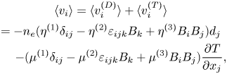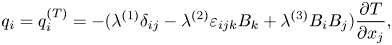We consider here terms in the heat flux and the electrical current produced by the temperature gradient only, so (2.1) and (2.2) can be written as

(2.4)\begin{gather} q_i=q_{i}^{(T)}=-(\lambda^{(1)}\delta_{ij}-\lambda^{(2)}\varepsilon_{ijk}B_k+\lambda^{(3)}B_i B_j) \frac{\partial T}{\partial x_j}, \end{gather}

(2.5)\begin{gather}\langle v_{i} \rangle=\langle v_{i}^{(T)} \rangle =-(\mu^{(1)}\delta_{ij}-\mu^{(2)}\varepsilon_{ijk}B_k+\mu^{(3)}B_i B_j) \frac{\partial T}{\partial x_j}. \end{gather}

Let us consider a plasma cylinder (see figures 1 and 2) with a uniform magnetic field $B$ along the $z$ axis, and a temperature gradient vector along the radius. In the case of a cylinder symmetry ${\partial }/{\partial z}={\partial }/{\partial \phi }=0$, the only non-zero parameters are $q_r, q_\phi, j_r, j_\phi, B_z$. Using the definition of the electrical current

(2.6)\begin{equation} j_i =-n_e e \langle v_i \rangle, \end{equation}

we obtain from (2.4) and (2.5) the following relations:

(2.7a–c)\begin{gather} q_r=-\lambda^{(1)}\frac{{\rm d} T}{{\rm d} r},\quad q_\phi=-B_z\left(\lambda^{(2)}\frac{{\rm d} T}{{\rm d} r}\right),\quad q_z =0, \end{gather}

(2.8a–c)\begin{gather}j_r=- e n_e\left(\mu^{(1)}\frac{{\rm d} T}{{\rm d} r}\right),\quad j_\phi=- en_eB_z\left(\mu^{(2)}\frac{{\rm d} T}{{\rm d} r}\right),\quad j_z=0. \end{gather}

Figure 1. Conducting cylinder with Hall current $j_{{\rm Hall}}$, depending on the magnitude of the radial temperature gradient and external constant magnetic field $B_0$ along its axis. The induced magnetic field $B_1$ is determined by the Hall current. Here $R_1$ is the radius of the central heated region with constant temperature $T_0$. The toroidal region, coloured in grey, contains Hall current and associated magnetic field, which has an opposite direction to the external field $B_0$, decreasing the resulting field along the cylinder.

Figure 2. The same cylinder as in figure 1, with opposite direction of the constant magnetic field $B_0$. We see that the magnetic field $B_1$, induced by Hall currents $j_{{\rm Hall}}$ is again opposite to the direction of $B_0$. Therefore, the resulting magnetic field decreases, for any direction of the magnetic field $B_0$.

Figures 1 and 2 have opposite directions of the initial magnetic field $B_0$. In both cases this field is deceasing due to the action of the Hall current. The same decrease of $B_z$ remains in the opposite direction of the heat flux, with heating of the outer boundary of the cylinder.

The Lorentz approximation is applied when the mass of light particles (electrons) is much smaller than the mass of heavy particles (ions or nuclei), and in addition electron–electron collisions are neglected. In this approximation the linearized Boltzmann equation, from which kinetic coefficients are derived, has an exact solution at zero magnetic field. In different approaches the solution in Lorentz approximation was considered by Chapmen & Cowling (1952) (p. 187), see also Schatzman (1958) and Bisnovatyi-Kogan (2001).

The explicit exact solution in Lorentz approximation is obtained for the case of a zero magnetic field. The heat flux connected only with the temperature gradient, is given in Schatzman (1958) and Bisnovatyi-Kogan (2001):

(2.9a,b)\begin{equation} q^T_i=-\tilde\lambda_T \frac{\partial{T}}{\partial x_{i}},\quad \tilde\lambda_T= \frac{320}{3{\rm \pi}}\frac{k^2 Tn_e}{m_e}\tau_e. \end{equation}

For the average velocity we can write the expression in the Lorentz approximation (Glushikhina 2020) with the thermal diffusion for the non-degenerate case:

(2.10a,b)\begin{equation} \langle v_i^{T}\rangle=-\mu^{l}\frac{\partial{T}}{\partial x_{i}},\quad \mu^{l}\equiv \frac{\sigma_T}{en_e} = \frac{16k}{m_e {\rm \pi}}\tau_e. \end{equation}

Using the expression for the electric current density, we obtain the thermodiffusion part in the form

(2.11)\begin{equation} j_i^T =-n_e e \langle v_i^T \rangle =-\sigma_T \frac{\partial T}{\partial x_i}. \end{equation}

We use here the parameters: electron Larmor frequency $\omega _B$; the time between $eN$ collisions $\tau _e$; and thermal electrical conductivity coefficient $\sigma _T$; which in the non-degenerate Lorentz gas approximation are determined as (Bisnovatyi-Kogan 2001)

(2.12)\begin{equation} \left.\begin{gathered} \omega_B=\frac{eB}{m_e c},\quad \tau_{e}=\frac{3}{4}\sqrt{\frac{m_e}{2{\rm \pi}}} \frac{(kT)^{3/2}}{Z^2{e}^4n_N\varLambda}, \\ \sigma_T = e n_e \mu_{e}=\frac{6\sqrt{2}}{{\rm \pi}^{3/2}\varLambda} \frac{e n_e k^2 T}{n_N e^4 Z^2}\left(\frac{kT}{m_e}\right)^{1/2} = \frac{16k e n_e}{m_e {\rm \pi}}\tau_e. \end{gathered}\right\} \end{equation}

Here $n_e, n_N$ are concentrations of electrons and nuclei with atomic number $Z$; $\varLambda$ is a Coulomb logarithm. The microscopic process of binary collision is not disturbed here by the magnetic field. For a very large magnetic field this approximation is not exact, but it does not change qualitatively the macroscopic behaviour of the system (Braginskii 1958a).

Components of the kinetic coefficient's tensor in the presence of the magnetic field can be expressed using the kinetic coefficient in Lorentz approximation. In particular for thermal electrical conductivity with a $B_z$ magnetic field, the conductivity along magnetic field lines is $\sigma _T$, and across magnetic field lines it is equal to $\sigma _T/(1+\omega _{B}^{2}\tau _{e}^{2})$ In the Hall direction, that is perpendicular to the plane defined by $B_z$ and $\partial T/ \partial x$ the conductivity is written as $\sigma _T \omega _{B} \tau _{e}/(1+\omega _{B}^{2}\tau _{e}^{2})$ (Chapmen & Cowling 1952) (p. 322, p. 338). Hence components of the electrical current density vector $\boldsymbol {j}$ in a cylinder with $B_z$ and temperature gradient vector along the radius are determined as

(2.13)\begin{equation} \left.\begin{gathered} j_r=-\frac{\sigma_T (\boldsymbol{\nabla}T)_r}{1+\omega_B^2\tau_e^2}, \\ j_\varphi=-\frac{(\sigma_T(\boldsymbol{\nabla}T)_r ) \omega_B\tau_e }{1+\omega_B^2\tau_e^2},\quad j_z=0. \end{gathered}\right\} \end{equation}

The connection of vectors $\boldsymbol {j_\phi }$ and induced field $\boldsymbol {B}$ is determined by the Maxwell equations.

3 Model description, solutions and results

From Maxwell equations we obtain the following relations for the magnetic field components in the cylinder:

(3.1a,b)\begin{equation} B_r=B_\varphi=0,\quad \frac{c}{4{\rm \pi}}\frac{{\rm d} B_z}{{\rm d} r}= \frac{\sigma_T(\boldsymbol{\nabla}T)_r \omega_B\tau_e }{1+\omega_B^2\tau_e^2}. \end{equation}

The magnetic field $B_z$ in the cylinder consists of the constant component $B_0$, created by external source, and the field $B_{1}$, created by electrical current inside the cylinder:

(3.2)\begin{equation} B_z=B_0+B_1. \end{equation}

Let us consider a stationary state of the cylinder with a constant radial heat flux $Q$. The radial heat flux density is written now as

(3.3)\begin{equation} q_r=\frac{Q}{2 {\rm \pi}r}=-\tilde\lambda_T\frac{(\boldsymbol{\nabla} T)_r}{1+(\omega_B \tau_e)^2}. \end{equation}

This equation should be solved in combination with the equation for $B_z$ written as

(3.4)\begin{equation} \frac{{\rm d} B_z}{{\rm d} r}=\frac{4 {\rm \pi}}{c}\frac{\sigma_T(\boldsymbol{\nabla}T)_r \omega_B\tau_e }{1+(\omega_B\tau_e)^2}. \end{equation}

Using $(\boldsymbol {\nabla } T)_r$ from (3.3), we obtain the dependencies of the magnetic field derivative on the temperature, using (1.1), in the form

(3.5)\begin{equation} \frac{{\rm d} B_z}{{\rm d} r} =-\frac{3 Q \omega_B \tau_e e}{10 kT c r}. \end{equation}

Equations (3.3) and (3.5) cannot be extended on the axis with $r = 0$ because of singularities at zero radius. It is suggested in this problem, that the only source of heat is situated near the axis of the cylinder, and is represented by a uniformly heated cylinder with radius $R_1 << R_0$, where $R_0$ is the outer radius of the cylinder.

Equations (3.3) and (3.5) are solved jointly under boundary conditions $B_z(R_1)=B_0, \quad T(R_0)=T_0$, at given parameter $Q$. Introducing non-dimensional Hall component $b_1$ as $B_1 = B_0 b_1$, taking into account the definition $\omega _{B} = {eB_z}/{m_e c} = {e(B_0 +B_1)}/{m_e c} = \omega _{B0} (1+ b_1)$ and $x = {r}/{R_0}$ we write the (3.5) in the form

(3.6)\begin{equation} \frac{{\rm d} b_1}{{\rm d}x}=- \frac{3 e Q \tau_e }{10 k c T B_{0} x} \omega_{B0} (1+ b_1). \end{equation}

Equation (3.3) may be written in the following form:

(3.7)\begin{equation} Q = \frac{-\tilde\lambda_T (\boldsymbol{\nabla} T)_{r} 2 {\rm \pi}r}{1+\omega^2_{B0} \tau^2_{e} (1+b_1)^{2}}. \end{equation}

Assuming in (3.6) constant ratio $\tau _e/T = F$, then (3.5) takes the form

(3.8)\begin{equation} \frac{{\rm d} b_1}{{\rm d}x}=-\frac{3 e Q F}{10 c k B_0 x }\omega_{B0}(1+b_1),\quad 1> x>x_1 = \frac{R_1}{R_0},\quad b_1(x_1) = 0. \end{equation}

The analytical solution of (3.8) is written as

(3.9a,b)\begin{equation} b_1 =\left(\frac{x_1}{x}\right)^{\gamma} - 1,\quad \gamma = \frac{3 e QF}{10 k c B_0}\omega_{B0}. \end{equation}

The value of $b_1$ is approaching $(-1)$ at $x_1 \to 0$. In the case of a plasma cylinder with parameters from (2.12), the equations (3.6) and (3.7), determining the Hall component $b_1$, are written as follows:

(3.10)\begin{equation} \left.\begin{gathered} \frac{{\rm d} b_1}{{\rm d}x}=- \frac{3 e Q}{10 k c B_0 x } \omega_{B0} (1+ b_1) C_1 T^{1/2}, \\ \frac{{\rm d} T}{{\rm d}x}=-\frac{1+ C_1^{2} T^{3} \omega_{B0}^2(1+b_1)^2}{2 {\rm \pi}x C_2 T^{5/2}} Q . \end{gathered}\right\} \end{equation}

The constants $C_1$ and $C_2$ are determined from relations

(3.11)\begin{gather} \tau _e = \frac{3(kT)^{3/2}}{4Z^2 e^4 n_N \varLambda}\sqrt{\frac{m_e}{2 {\rm \pi}}} = C_1T^{3/2}, \end{gather}

(3.12)\begin{gather}\tilde \lambda_T = \frac{20 kT\sigma_T}{3 e} = \frac{40 \sqrt{2} k n_e}{{\rm \pi}^{3/2}\varLambda n_N}\left( \frac{kT}{e^2 Z}\right)^{2} \left( \frac{kT}{m_e} \right)^{1/2} = C_2 T^{5/2} \end{gather}

so that

(3.13a,b)\begin{equation} \omega_B=\omega_{B0}(1+b_1),\quad \omega_{B}\tau_e=C_1 T^{3/2}\omega_{B0}(1+b_1). \end{equation}

Let us introduce dimensionless parameters:

(3.14a–d)\begin{equation} {\tilde T}=\frac{T}{T_0},\quad N = \frac{3 e Q\omega_{B0} C_1}{10 kcB_0}T_0^{1/2},\quad G = C_1^{2} T_0^3 \omega_{B0}^{2},\quad E=\frac{2{\rm \pi} C_2 T_0^{7/2}}{Q}. \end{equation}

Equations (3.10) have following form with new parameters:

(3.15a,b)\begin{equation} \frac{{\rm d} b_1}{{\rm d}x} =-N\frac{(1+b_1){\tilde T}^{1/2}}{x},\quad \frac{{\rm d}\tilde T}{{\rm d}x}=-\frac{1+G (1+b_1)^2 {\tilde T^3}}{x E {\tilde T^{5/2}}}. \end{equation}

We solve (3.13a,b) numerically in the interval $x_1\leq x\leq 1$ at boundary conditions

(3.16a,b)\begin{equation} b_1(x_1) = 0,\quad \tilde T(x_1) = 1. \end{equation}

Results of the solution are presented in the figures 3–8 for the case of plasma parameters in the NS crust.

Figure 3. Magnetic field in the cylinder, induced by the Hall current, for $F = 5.2\times 10^{-5}$, $E = 0.012$ and three values of $N$: $N_1 = 6.0$; $N_2 = 0.6$; $N_3 = 6.0\times 10^{-2}$. These values are related to $Z = 26$, and include combinations $B_{0} = 10^{12}\ \textrm {G},\ T_0 = 10^{9}\ \textrm {K},\ \rho _0 = 10^{7}$ g cm$^{-3}$ for $N_1$; $B_{0} = 10^{13}\ \textrm {G}, T_0 = 10^{9}\ \textrm {K},\ \rho _0 = 10^{8}$ g cm$^{-3}$ for $N_2$; $B_{0} = 10^{14}\ \textrm {G},\ T_0 = 10^{9}\ \textrm {K}, \rho _0 = 10^{9}$ g cm$^{-3}$ for $N_3$.

Figure 4. Temperature distribution in the cylinder for the same parameters as in figure 3.

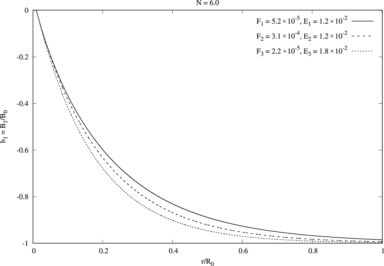
Figure 5. Magnetic field in the cylinder, induced by the Hall current, for $N = 6$ and three variants: $F_1 = 5.2\times 10^{-5},\ E_1 = 0.012$; $F_2 = 3.1\times 10^{-4},\ E_2 = 0.012$; $F_3 = 2.2\times 10^{-5},\ E_3 = 0.018$. These values are related to $Z = 26$, and include combinations $B_{0} = 10^{12}\ \textrm {G},\ T_0 = 10^{9}\ \textrm {K},\ \rho _0 = 10^{7}$ g cm$^{-3}$ for $F_1$, $E_1$; $B_{0} =10^{13}\ \textrm {G},\ T_0 = 1.8\times 10^{9}\ \textrm {K}, \rho _0 = 10^{8}$ g cm$^{-3}$ for $F_2$, $E_2$; $B_{0} = 10^{13}\ \textrm {G},\ T_0 = 3.5\times 10^{9}\ \textrm {K},\ \rho _0 = 10^{9}$ g cm$^{-3}$ for $F_3$, $E_3$.

Figure 6. Temperature distribution in the cylinder for the same parameters as in figure 5.

Figure 7. Magnetic field in the cylinder, induced by the Hall current, for $E=0.012$, and three variants: $F_1=5.1\times 10^{-3},N_1=6.0$; $F_2=5.1\times 10^{-5},N_2=0.6$; $F_3=5.1\times 10^{-7},\ N_3 =0.06$. These values are related to $Z = 26$, and include combinations $B_{0} = 10^{13}\ \textrm {G},\ T_0 = 10^{9}\ \textrm {K},\ \rho _0 = 10^{7}$ g cm$^{-3}$ for $F_1$, $N_1$; $B_{0} =10^{13}\ \textrm {G},\ T_0 =10^{9}\ \textrm {K},\ \rho _0 = 10^{8}$ g cm$^{-3}$ for $F_2$, $N_2$; $B_{0} = 10^{13}\ \textrm {G},\ T_0 =10^{9}\ \textrm {K},\ \rho _0 = 10^{9}$ g cm$^{-3}$ for $F_3$,$N_3$.

Figure 8. Temperature distribution in the cylinder for the same parameters as in figure 7.

Equation (3.13a,b) can be used for analysing the magnetized plasma in laboratory facilities. Results of these calculations are presented in the figures 9–14.

Figure 9. Magnetic field in the cylinder, induced by the Hall current, for $F=1.2\times 10^{-5}$, $E=0.1$, and three variants: $N=0.8$; $N_2=8.5$; $N_3=85.2$. These values are related to $Z =1$ and include combinations $B_{0} = 5\times 10^3$ G, $T_0 =2\times 10^{5}$ K, $\rho _0=10^{-4}$ g cm$^{-3}$ for $N_1$; $B_{0}=5\times 10^{2}$ G, $T_0 = 2\times 10^{5}$ K, $\rho _0 = 10^{-5}$ g cm$^{-3}$ for $N_2$; $B_{0}=50$ G, $T_0 = 2\times 10^{5}$ K, $\rho _0=10^{-6}$ g cm$^{-3}$ for $N_3$.

Figure 10. Temperature distribution in the cylinder for the same parameters as in figure 9.

Figure 11. Magnetic field in the cylinder, induced by the Hall current, for $E = 0.1$ and three variants: $F_1= 1.3\times 10^{-11}$, $N_1=0.085$; $F_2=1.3\times 10^{-9}$, $N_2=0.8$; $F_3=1.3\times 10^{-7}$, $N_3=8.5$. These values are related to $Z = 1$, and include variants $T_0 = 2\times 10^{5}$ K, $B_{0}= 50$ G, $\rho _0=10^{-3}$ g cm$^{-3}$ for $N_1$, $F_1$; $\rho _0 = 10^{-4}$ g cm$^{-3}$ for $N_2$, $F_2$; $\rho _0 = 10^{-5}$ g cm$^{-3}$ for $N_3$ $F_3$.

Figure 12. Temperature distribution in the cylinder for the same parameters as in figure 11.

Figure 13. Magnetic field in the cylinder, induced by the Hall current, $N = 0.8,\ E=0.1$ and three variants: $F_1 = 4.7\times 10^{-5}$; $F_2 = 4.7\times 10^{-7}$; $F_3 = 4.7\times 10^{-9}$. These values are related to $Z = 1$, and include variants $\rho =10^{-4}$ g cm$^{-3}$, $T_0 = 2\times 10^{5}\ \textrm {K}$, $B_{0} = 10^{4}$ G, for $F_1$; $B_{0} =10^{3}$ G, for $F_2$; $B_{0} =10^{2}$ G, for $F_3$.

Figure 14. Temperature distribution in the cylinder for the same parameters as in figure 13.

4 Discussion

It is shown in this paper that the magnetic field, generated by the azimuthal Hall current, decreases the magnetic field, produced by external sources. Equation (3.15), determining $B_1/B_0$ ratio of the magnetic field produced by the Hall current to the external magnetic field, is derived. Hall current in the present consideration is produced by a temperature gradient for the case when the diffusion vector is equal to zero (Bisnovatyi-Kogan & Glushikhina 2018a,b; Glushikhina 2020). Analytical results are obtained for the case, when coefficients of heat conductivity, electroconductivity and a time between collisions are constant. Results of numerical calculations performed for the case of plasma parameters in NS envelopes, are shown in figures 3–14. The calculations for parameters, related to laboratory plasma, are presented in figures 9–14.

Kinetic coefficients in the magnetic field are determined by tensors, connected with a temperature gradient and a diffusion vector. Influence of the Hall current on the temperature distribution, structure of magnetic and electric fields, in realistic geometry of a NS envelope needs further consideration. It can be important for modelling of the structure of the magnetic field along the surface of the NS, and for studying a coupled magnetothermal evolution of temperature, magnetic and electric fields in NSs. The electrons in the inner envelope of the NS may become degenerate and relativistic in conditions of high density and temperature. We have used non-relativistic and non-degenerate approximation for transport coefficients in all our calculations. Therefore, the results presented in figures 3–8 can be considered as correct only qualitatively. Account of relativistic corrections and degeneracy in calculations of transport coefficients of plasma meets with difficulties, so analytical formulae for these conditions have been obtained approximately, with considerable simplifications. In the situation, when the structure of the NS is far from a very simple cylindrical model, used here, we have done calculations of the nonlinear Hall effects using simplified transport coefficients for NS parameters.

In recent years experimental study of astrophysical processes is developing (laboratory astrophysics). The goal is to model astrophysical processes in a terrestrial laboratory, based on the similarity theory relations. Our results can be useful for studying the Hall current effects in the laboratory plasma, which may be applied for astrophysical conditions. High temperature gradients in the presence of very strong magnetic fields are formed during stellar core collapses, leading to formation of NSs, accompanying supernovae explosions. The newborn NS is very hot, strongly magnetized and with large temperature gradients. Thermoelectric processes are very important on this short (few years) stage of the NS's life, during a rapid cooling by neutrino energy losses (Tsuruta & Cameron 1965). The magnetic field structure formed in this short stage keeps it frozen, and the time of its slow changes may exceed millions of years.