Introduction
Several ice flow models of increasing orders of complexity have been developed to model the dynamics of ice- sheet systems (Reference HutterHutter, 1982; Reference BlatterBlatter, 1995; Reference PattynPattyn, 2003; Reference HindmarshHindmarsh, 2004). All these models are derived from the same momentum-balance and incompressibility equations, i.e. the full-Stokes equations, using an appropriate simplifying kinematics hypothesis. Several studies describe the model properties and their domain of validity (Reference HindmarshHindmarsh, 2004; Reference GudmundssonGudmundsson, 2008; Reference Dukowicz, Pric and LipscombDukowicz and others, 2010; Reference Morlighem, Rignot, Seroussi, Larour, Ben Dhia and AubryMorlighem and others, 2010; Reference Schoof and HindmarshSchoof and Hindmarsh, 2010). Simplified flow models reduce the computational cost by simplifying the ice dynamics and make it possible to run large-scale simulations with limited computational resources (Reference MacAyealMacAyeal, 1992; Reference Marshall and ClarkeMarshall and Clarke, 1997). Higher-order models allow a better representation of the ice dynamics, but at a higher computational cost. More importantly, however, the gain in precision from these models depends on the flow regime of the ice. In some regions, the gain in precision of higher-order models may be significant or critical (e.g. near the grounding line of a glacier or near an ice divide). But in other regions, the gain in precision may not be significant at all. Hybrid models that combine different orders of complexity in different regions are therefore highly desirable, because they offer a compromise between capturing the correct dynamics in critical regions while minimizing the computational cost.
Hybrid modeling has been used by Reference Hulbe and MacAyealHulbe and MacAyeal (1999) to model the West Antarctic ice sheet. This evolutive thermodynamic model couples inland-ice, ice-stream and ice-shelf dynamics using the shallow-ice approximation (SIA) for the inland ice (Reference HutterHutter, 1982) and the shelfy-stream approximation (SSA) for ice streams and ice shelves (MacAyeal, 1989).
Reference Pollard and DeContoPollard and DeConto (2009) used the same approximations to model the evolution of the Antarctic ice sheet during the last 5 × 10⁶ years, with SIA for grounded ice and SSA for floating ice. As longitudinal stresses are not included in the SIA, the two models cannot be directly coupled, and are solved consecutively. In order to capture the grounding-line effects, Reference Pollard and DeContoPollard and DeConto (2009) used a mass-flux constraint at the transition between the two models (Reference SchoofSchoof, 2007). This mass-flux condition enables ice mass- flux continuity at the transition between the two models, but does not correspond to a two-way coupling between them.
Another approach to hybrid modeling (Reference Bueler and BrownBueler and Brown, 2009) combines SSA and SIA simultaneously everywhere on the glacier. SSA is used as a sliding law for SIA and a parameter is adjusted to balance the amount of ice motion due to SSA and SIA, from pure SSA on floating parts of the ice- sheet domain, to pure SIA when ice is frozen at the bedrock interface.
These models can be considered a first step toward introducing a new generation of hybrid models in ice-sheet modeling; here we propose a method to go a step further. We present a new technique, inspired by the Arlequin framework (Reference Ben DhiaBen Dhia, 1998; Reference Ben Dhia and RateauBen Dhia and Rateau, 2001, 2005), to strongly couple mechanical models of varying orders of complexity, in particular, of higher complexity than the models described above. First, we discuss the basic ice flow models and how we implemented them. These models are (1) a two-dimensional (2-D) SSA; (2) a three-dimensional (3-D) higher-order (HO) model; and (3) the full-Stokes (FS) model. We then describe the new coupling technique, called the Tiling method, to couple SSA, HO and FS. We demonstrate its use on synthetic geometries, discuss the results and draw conclusions on the use of the Tiling method in ice-sheet flow modeling and its extension to transient models.
Methods
Ice flow equations
Ice flow models are all derived from the same classical momentum-balance equation, where acceleration and Cori-olis effects are considered negligible:
where ∇ · σ is the divergence vector of the stress tensor, σ, ρ the ice density and g the acceleration due to gravity. Ice is considered incompressible and the continuity equation reads:
Where ![]() is the trace of the strain-rate tensor,
is the trace of the strain-rate tensor, ![]() . As ice is being treated as a viscous incompressible material (e.g. Reference Cuffey and PatersonCuffey and Paterson, 2010) its behavior law only involves the deviatoric stress and we introduce the pressure, p, as a Lagrange multiplier to ensure that the equation of incompressibility is satisfied:
. As ice is being treated as a viscous incompressible material (e.g. Reference Cuffey and PatersonCuffey and Paterson, 2010) its behavior law only involves the deviatoric stress and we introduce the pressure, p, as a Lagrange multiplier to ensure that the equation of incompressibility is satisfied:
where µ is the viscosity (scalar as the ice is assumed to be isotropic) and σ′ the deviatoric stress tensor such that σ′ = σ + pI, with I the identity tensor. The viscosity follows Glen’s flow law (Reference GlenGlen, 1955), a particular type of Norton- Hoff law:

Where ![]() is the effective strain rate, n is Glen’s coefficient, usually taken as n = 3 (Reference Cuffey and PatersonCuffey and Paterson, 2010), and B is the ice hardness. Equations (1–4) are strong equations set in the domain occupied by the ice and denoted Ω.
is the effective strain rate, n is Glen’s coefficient, usually taken as n = 3 (Reference Cuffey and PatersonCuffey and Paterson, 2010), and B is the ice hardness. Equations (1–4) are strong equations set in the domain occupied by the ice and denoted Ω.
Boundary conditions
The air pressure being negligible, a stress-free condition is applied at the upper surface:
with n the outward unit normal to the boundary of the glacier. Water pressure is applied at the ice/water interface (including the ice front, Γi):
where ρw is the water density and z the elevation with respect to sea level. At the ice/bedrock interface we specify the normal velocity and the tangential force. A Weertman friction law (Reference Cuffey and PatersonCuffey and Paterson, 2010) is applied to model basal friction:
where τb= (σ · n)|| are the tangential components of external forces, vb the tangential velocity at the ice/bedrock interface and α a friction coefficient. We ensure that no ice penetrates into the bedrock using a non-interpenetration condition at this ice/bedrock interface: the velocity normal to the ice/bedrock interface is set to zero. We use non- homogeneous Dirichlet boundary conditions based on the observed velocity for the rest of the border (lateral boundaries where there is no ice front).
Common approximations
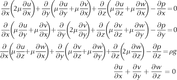
We use Cartesian coordinates, (x, y, z), with z the vertical axis, and write (u, v, w) for the three components of the velocity vector, u. The FS approach directly solves Eqns (1) and (2) with no simplification. For an incompressible material in terms of velocity components, this system, set in Ω reads:

A simplified 3-D model derived from these equations, known as the higher-order model (HO) (Reference BlatterBlatter, 1995; Reference PattynPattyn, 2003), makes two assumptions: (1) the horizontal gradients of vertical velocities are negligible compared to the vertical gradients of horizontal velocities:
and (2) the bridging effect (Reference Van der Veen and WhillansVan der Veen and Whillans, 1989) is neglected so the third equation of the full-Stokes system, set in Ω, reduces to

Using these assumptions in the momentum equations, the horizontal vector-valued velocity field is decoupled from the vertical component and the pressure. It is a solution of

where s is the ice upper surface elevation.
The 2-D shallow-shelf or shelfy-stream approximation (SSA) was first derived from the full-Stokes equations (Eqns (8)) by MacAyeal (1989). In addition to the assumptions made for HO, vertical shear is neglected:
Using these assumptions, the horizontal components of velocity, u and v, do not depend on z. Integration from the bed to the surface, set in the mean section ω of Ω, gives the model equations

where H is the ice thickness, ![]() the depth-averaged viscosity, (τbx
, τby) the components of τb and δsheet a function equal to 1 on the ice sheet and 0 on the ice shelf. The basal friction is generally assumed to be horizontal only, which gives τbx = -α2 u and τby = -α2
v.
the depth-averaged viscosity, (τbx
, τby) the components of τb and δsheet a function equal to 1 on the ice sheet and 0 on the ice shelf. The basal friction is generally assumed to be horizontal only, which gives τbx = -α2 u and τby = -α2
v.
In the SSA and HO models, the equations are decoupled and the vertical velocity is computed separately by solving the incompressibility equation (Eqn (2)) once the horizontal components are known.
SIA is not discussed in our study because it neglects lateral shear. The mechanical equations of a region treated with SIA are consequently not affected by changes that take place in another region and hence no coupling method is necessary to compute the velocities of such areas.
Numerical implementation
All these models are implemented in the massively parallelized finite-element Ice Sheet System Model (ISSM) (Reference Morlighem, Rignot, Seroussi, Larour, Ben Dhia and AubryMorlighem and others, 2010; Reference Larour, Seroussi, Morlighem and RignotLarour and others, 2012). We use MINI prismatic elements (Reference Gresho and SaniGresho and Sani, 2000) for FS to fulfill the compatibility Ladyzhenskaya-Babuška-Brezzi condition. We employ linear P1 triangular elements for SSA and P1 prismatic elements for HO.
These three models (SSA, HO and FS) rely on a nonlinear behavior law (Eqn (4)) and we use a fixed-point or Picard's method (Reference ReistReist, 2005) to solve them (Fig. 1).

Fig. 1. Convergence algorithms used for SSA or HO (left) and FS (right).
The finite-element implementation of the models described above relies on the variational/weak formulations of their respective field equations, associated with their boundary conditions. Subscripts s, p and m refer to FS, HO and SSA, respectively. Let Vs, Vp and Vm be the kinematically admissible fields associated with these problems. The variational formulations for the three problems are, respectively, find us ∈ Vs, u p ∈ Vp and u m ∈ Vm such that
The expressions of the bilinear forms, a s, a p and a m, as well as the linearforms, l s, l p and l m, are detailed in the Appendix. These forms respectively represent the virtual work of internal and external forces (e.g. Reference Zienkiewicz and TaylorZienkiewicz and Taylor, 1989, for more details on the finite-element method).
Tiling method
The three aforementioned models represent three levels of complexity that do not require the same computational resources. We wish to couple these different models of ice flow to minimize the computational cost, while maintaining accuracy. Developing new techniques for coupling models and scales of complex mechanical or physical problems is an active research area in the fields of computational mechanics and physics.
The method we present here is inspired by the Arlequin framework developed by Reference Ben DhiaBen Dhia (1998) (see also Reference Ben Dhia and RateauBen Dhia and Rateau, 2005). It is based on a blending zone where two different models are strongly blended, hence the name Tiling method. Here we outline the main ideas of this approach by considering a generic problem.
Let Ω be the model domain and V the set of kinematically admissible fields for Ω. We write a and I the bilinear and linearforms associated with the variational formulations, and a Ω and I Ω their restriction to Ω. The generic problem to solve is:
Instead of solving this mono-model problem with the finite-element method, the idea is to first reformulate the problem using a domain decomposition. We consider two subdomains of Ω, denoted Ω1 and Ω2, such that
These two subdomains overlap in a transition zone. The overlapping region, denoted Ωt, is called the blending zone or superposition zone. It is defined by (Fig. 2)
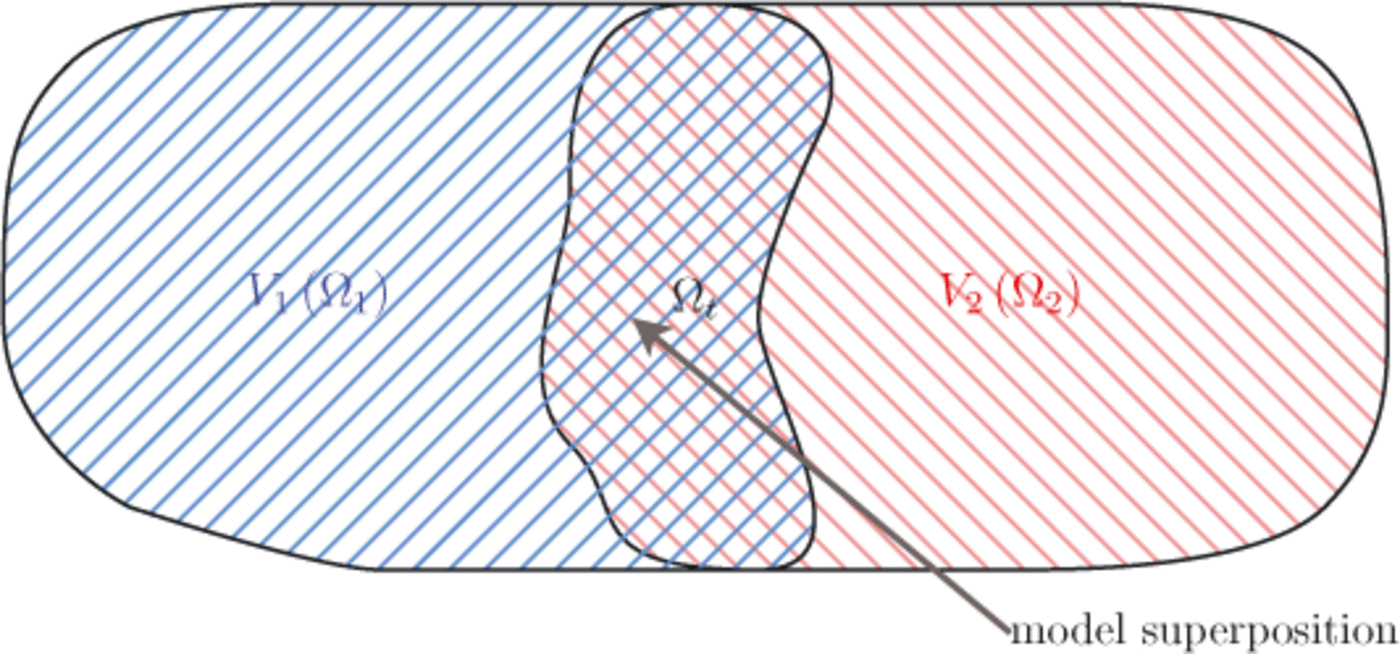
Fig. 2. Separation of the domain into two subdomains.
Let V 1 and V 2 be the sub-spaces of kinematically admissible fields for the two subdomains, such that V = V 1 + V 2. The solution, u , is taken as the sum of the contributions of velocity from the two subdomains (Fig. 3):

Fig. 3. Example of solution in one dimension. The solution u is the sum of u1 and u2 on the blending zone. Homogeneous Dirichlet conditions are imposed on the border of the blending zone following Eqn (21).

In order to have a continuous solution, u , we need to impose additional boundary conditions on the boundary of the blending zone, ∂Ωt. All points on ∂Ωt have homogeneous Dirichlet conditions for one of the two contributions (Fig. 3). For the sake of simplicity, and without limiting the extent of the method, we detail here these additional Dirichlet conditions in the specific case where one subdomain is strictly embedded in Ω, i.e. no node of this first subdomain is on the border of the domain, ∂Ω. Under these conditions, the additional Dirichlet conditions (Fig. 3) are

The kinematically admissible fields are now

If we use the bilinearity of a, the linearity of l, and if we decompose the test function, φ, on the two spaces, the problem formulation using the domain decomposition becomes:


The coupling terms allow the coupling of u 1 and u 2 in the blending zone.
The basic idea of the Tiling method consists of taking advantage of this new formulation to introduce two different mechanical models on the two subdomains, Ω1 and Ω2. Schematically, let a 1,Ω1 , a 2,Ω2 and l 1,Ω1 , l 2,Ω2 be the bilinear and linear forms associated with the variational formulations of the two mechanical models in their respective domains. Let a 1−2,Ωt and a 2−1,Ωt be the transition blending bilinear forms in the transition domain, Ωt. We define a weak multimodel formulation associated with the Eqn (23) problem by:

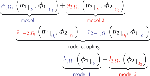
We see that the final formulation is the sum of the two mono-model formulations and there are two additional coupling terms, a 1−2,Ωt ( u 1,ϕ 2 ) and a 2−1,Ωt ( u 2,ϕ1 ), on the left-hand side. These terms, which will be detailed for the coupling of different models, are nonzero only for the elements inside the blending zone, where both u 1 and u 2 are simultaneously nonzero. In the blending zone, the two models are employed simultaneously. The additional terms that combine the models in Eqn (24) ensure the continuity of the solution and the two-way coupling. Elements outside this zone are treated as mono-model.
This method is easily parallelizable and requires limited modifications of an existing code, as the additional coupling terms must be taken into account only in the blending zone. However the continuous problem is singular because of the existence of the volume blending zone where the two models are used simultaneously, leading to an infinite redundant set of equations. We take advantage of the problem discretization to overcome this redundancy problem.
Domain discretization
In order to tackle the redundancy issue for finite-element discretization of the continuous problem, Eqn (24), our basic idea consists of reducing the blending zone to only ‘one layer’ of elements, so that all nodes of Ωt are on the border of this zone, ∂Ωt. Each node is associated with only one modelexcept on ∂Ωt, where one of the two models is constrained. Therefore, u1 and u2 are never simultaneously computed on the same node. Under these conditions, the discretized problem is regular. This domain discretization is necessary to avoid having multiple solutions of the same continuous problemand therefore guarantees uniqueness of the solution
Coupling the shelfy-stream approximation (SSA) with higher-order (HO) models
SSA and HO solve the same system of decoupled equations the latter with a 3-D model and the former with a 2-D depthintegrated model. Coupling them with the Tiling method is relatively straightforward, even if some adjustments must be made at the 2-D/3-D transition
Let Ωm be the domain where SSA is applied, and Ωp the HO domain, Ωm and Ωp being a partition of Ω in the sense of Eqns (18) and (19). First, homogeneous Dirichlet conditions must be added as specified in the previous section:
where u m is the velocity associated with SSA, and u p the velocity associated with HO.
Second, two different models coexist in the transition zone and special care must be given to the treatment of ice viscosity in this area. Indeed, the viscosity depends on the effective strain rate (Eqn (4)) and this strain rate is not constant with depth in the transition zone because of the contribution of HO. We use the most general viscosity law, the one used in HO, for both models in the blending zone, µ (u) = µ (u m + u p).
Coupling the higher-order (HO) model with full-Stokes (FS) formulations
Let Ωp be the domain where HO is applied and Ωs the FS domain. The coupling between FS and HO is more challenging than that between SSA and HO. FS solves the three components of the velocity and the pressure, whereas HO decouples the horizontal and vertical components of the velocity Coupling FS to HO horizontal equations therefore ensures the continuity of u and v, but not of w. To ensure the continuity of the vertical velocity, we must include a vertical velocity component in HO that is coupled to FS in the blending zone. We use an iterative algorithm with an a priori estimate of the HO vertical velocity, which is updated at each iteration using the incompressibility equation, so that vertical and horizontal velocities of HO remain consistent. The pressure, being a Lagrange multiplier, cannot be constrained on the boundary of the blending zone. It is therefore left free for the entire domain, Ωs. The additional boundary conditions are
where (u s, v s, w s) and (u p, v p, w p) are the velocity components of HO and FS, respectively. Let ϕp and ϕs be kinematically admissible fields for HO and FS. For each iteration of the viscosity, the equation to solve is

where a
p and a
s are the bilinear forms associated with HO and FS, l
p and l
s the linear forms associated with HO and FS. ![]() are the transition blending bilinear forms in the transition domain, Ωt. u
s is the velocity and pressure of
are the transition blending bilinear forms in the transition domain, Ωt. u
s is the velocity and pressure of ![]() are the horizontalvelocity of HO and FS (respectively
are the horizontalvelocity of HO and FS (respectively ![]() and w
p the horizontal and vertical velocities of HO extended with zeros so that they become FS kinematically admissible (respectively (u
p, v
p, 0, 0) and (0, 0, w
p, 0)).
and w
p the horizontal and vertical velocities of HO extended with zeros so that they become FS kinematically admissible (respectively (u
p, v
p, 0, 0) and (0, 0, w
p, 0)).
In this configuration, coupling terms are added both to the left-hand side to couple ![]() to FS terms and on the right-hand side to ensure the continuity with w
p.
to FS terms and on the right-hand side to ensure the continuity with w
p.
To update the vertical velocity of HO, the incompressibility equation must be solved in the HO part of the domain, including the blending zone. The incompressibility equation must be satisfied for the total velocity, sum of FS and HO:

The schematic in Figure 4 summarizes how these iterations are performed and how the a priori vertical velocity is updated.

Fig. 4. Scheme representing the iterations done for a hybrid FS/HO
model.
Coupling the shelfy-stream approximation (SSA) with full-Stokes (FS) solutions
Coupling SSA to FS combines the problems encountered in the two previous couplings. In the blending zone, we use a viscosity, µ, that varies with depth, even for SSA. The horizontal equations of SSA and FS equations are solved simultaneously, which ensures continuity of the horizontal velocity We use an a priori estimate of the vertical velocity for SSA, which is updated at each iteration of the viscosity, similarly to that done for HO/FS coupling (Fig. 4).
Applications
To validate the method, we first verify that the Tiling method is consistent when coupling one model to itself (e.g. SSA with SSA or FS with FS). Results found when coupling each model to it self are exactly identical to mono-model results.
There are some configurations for which all three approximations (SSA, HO and FS) are valid and yield the same results. The results performed with hybrid models must be similar to results found with mono-models. Here we use a 1000 km long square ice shelf in hydrostatic equilibrium, in which the thickness varies between 1000 and 300 m at the ice front. We constrain the velocity (homogeneous Dirichlet conditions) on three edges, and water pressure is applied on the fourth edge to simulate an ice front. We use three different models: SSA, HO and a hybrid SSA/HO model. In the hybrid model, SSA elements are used on the left half and HO elements on the right half; a layer of elements combines both approximations at the transition. Figure 5 shows horizontal surface velocity components for the three models. Both components are identical for SSA and HO, as well as for the hybrid model. On the hybrid model (Fig. 5b and e), the blending is impossible to detect visually.
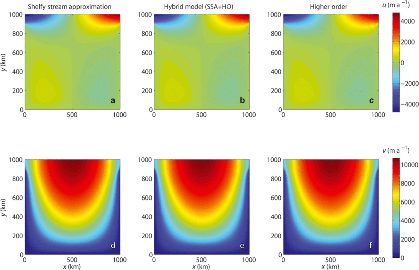
Fig. 5. Top view of velocity components of a square ice shelf for three ice flow models: SSA, HO and a hybrid SSA/HO model. (a) u for
SSA; (b) u for hybrid; (c) u for HO; (d) v for SSA; (e) v for hybrid; (f) v for HO.
In a second experiment, we test the ability of the Tiling method to combine models. This experiment consists of an ice flow over a flat bed. The ice sheet is 1000 km long and 500 m thick on average. Similarly to the previous experiment, we constrain the velocity (0 and 100 ma-1 in the x and y directions, respectivity) on three edges and apply water pressure on the fourth edge. Next to the ice front, a very rough bed is introduced, with bumps and hollows whose typical length scale is equal to one ice thickness (Fig. 6). This experiment is useful for testing the Tiling method, as HO and FS do not yield the same results; HO (Fig. 7d and g) is nearly unaffected by the rough bed, contrary to FS (Fig. 7f and i), as some 3-D effects are captured by this model. The difference in velocity between the two models varies between 50 and 100 ma-1 at the ice front and decreases upstream. A hybrid model that combines FS elements on and around the rough bed area, and HO on the rest of the domain is employed (Fig. 7b). The velocity computed with the hybrid model (Fig. 7e and h) is almost identical to the FS velocity, and the model transition is seamless. The computational time is 15.7 s for the HO model, 70.3 s for the FS model and 23.7 s for the hybrid model. Since the area over which FS is applied is spatially limited, the number of degrees of freedom is reduced considerably. As a result, the hybrid model is significantly faster than a pure FS model.
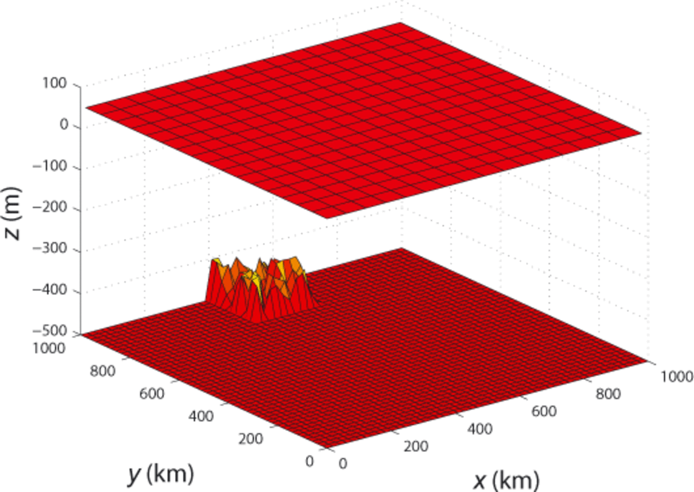
Fig. 6. Geometry of the rough bed experiment showing the rough bed close to the ice front and the flat upper surface.
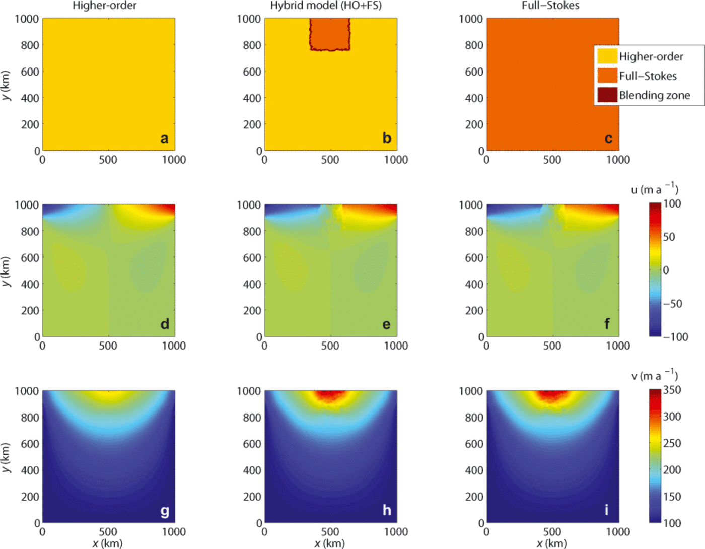
Fig. 7. Top view of the square ice sheet, showing the type of model applied and the velocity components for three ice flow models: HO, FS and hybrid model (HO/FS) using a polar stereographic projection. The type of elements is vertically extruded so it is similar for each element of the column. (a) Type of elements used for HO; (b) type of elements used for hybrid; (c) type of elements used for FS; (d) u for HO; (e) u for hybrid; (f) u for FS; (g) v for HO; (h) v for hybrid; (i) v for FS.
Discussion
Using simplifications of the ice flow equations reduces the computational time required to run numerical models, which is useful for large-scale modeling, but it has been shown that these approximations fail to reproduce certain critical aspects of ice dynamics. It is therefore essential to first determine where each model is valid, and where sophisticated models are required.
Reference HindmarshHindmarsh (2004) and Reference GudmundssonGudmundsson (2008) describe the effects of small-amplitude perturbations in boundary data to ice flow solutions. They show that SIA correctly reproduces the effect of long-wavelength perturbations at low slip ratios. Higher-order approximations that include longitudinal stress improve the accuracy of the results and can be used at smaller wavelengths. For wavelengths smaller than about five ice thicknesses (depending on other parameters like slip ratios) no approximation is able to reproduce FS correctly It has also been shown that modeling of grounding-line dynamics, a fundamental aspect of glacier flow dynamics, requires sophisticated, higher-order models (Reference Vieli and PayneVieli and Payne, 2005; Reference Nowicki and WinghamNowicki and Wingham, 2008; Reference Durand, Gagliardini, Zwinger, Le Meur and Hind-marshDurand and others, 2009; Reference Morlighem, Rignot, Seroussi, Larour, Ben Dhia and AubryMorlighem and others, 2010). Devising criteria that define the area of validity for each approximation of the FS equations is still an active area of research.
The Tiling method is a numerical technique that enables a strong coupling of different approximations of the ice flow equations by constructing hybrid models that combine different mechanical models. Its simplicity and ease of implementation in existing codes makes it an invaluable technique for continental-scale modeling, as it allows use of computationally expensive models only where they are required. The successful application of the Tiling method on the rough bed experiment shows that it is possible to correctly capture the dynamics that only sophisticated models can reproduce in critical areas, while reducing the computational time by using simpler models where they are valid. With the Tiling method implemented in ISSM (Reference Morlighem, Rignot, Seroussi, Larour, Ben Dhia and AubryMorlighem and others, 2010, Reference Morlighem, Rignot, Seroussi, Larour, Ben Dhia and Aubry2011; Reference SeroussiSeroussi and others, 2011; Reference Larour, Seroussi, Morlighem and RignotLarour and others, 2012), it is possible to envision a continental modeling of Greenland or Antarctica that only uses sophisticated models in the grounding- line regions, and simplified models elsewhere. With our current computational resources, it is not practical to run FS simulations of ice-sheet flow in Antarctica at high resolution.
In this paper, we have relied on a direct solver: MUMPS (MUltifrontal Massively Parallel sparse direct Solver). When using iterative solvers, one should use block-preconditioning to make sure that each subdomain is properly conditioned. This will improve the scalability of the problem. We expect the gain in computational time to increase in such cases.
All the applications presented in this paper are diagnostic simulations (fixed geometry), in which only the velocity is computed. However, this technique can be easily extended to transient simulations. The coupling in the stressbalance equation induced by the Tiling method does not change the way in which the energy-balance and mass- balance equations are solved. The Tiling method enables computation of a 3-D velocity field that incorporates contributions from both models that can be directly used in the thermal- or mass-transport equations, regardless of the coupling. The velocity in the energy-balance and mass- transport models is simply taken as the total velocity in the case of the hybrid model. Solving for the ice velocities is generally the most time-consuming component of a transient model, as it involves the largest number of degrees of freedom and requires solving a nonlinear problem. The gains made in computational time by using a hybrid model approach to solve for the ice velocity will directly improve the overall efficiency of transient simulations.
We expect this method to treat the problem of grounding- line migration more efficiently. The area where FS is applied can be spatially limited to the grounding-line region, as FS is required to resolve the position of the grounding line using a contact approach (Reference Nowicki and WinghamNowicki and Wingham, 2008; Reference Durand, Gagliardini, Zwinger, Le Meur and Hind-marshDurand and others, 2009).
The potential utility of hybrid models that combine these approximations is significant. FS is needed in some critical areas, but current computational resources do not always allow for its use at a continental scale. Hybrid models have the potential to greatly improve physical accuracy, despite computational resource constraints, by combining models in their domain of validity, while preserving computational cost. Moreover, we see that the hybrid model behaves 'better' than a pure FS model. The FS equations are saddle-point problems that lead to symmetric but indefinite stiffness matrices in the finite-element formulation, contrary to simpler models that produce positive definite matrices. Solving for large saddle-point problems requires the use of, for example, Krylov subspace methods, that converge slowly and are more prone to failure. FS models are therefore numerically less stable than simpler models that do not rely on a mixed formulation (Reference DukowiczDukowicz, 2012; Reference Perego, Gunzburger and BurkardtPerego and others, 2012). Furthermore, it is difficult to run a FS model on real geometries, because it can quickly diverge from the initial state if the mesh is too coarse in some regions, or if the configuration changes too rapidly. Simpler models are more robust. Thus, hybrid models have the potential to improve robustness by limiting the areas over which FS is employed.
The next step is to improve our knowledge and understanding of these ice flow models, their domain of validity in particular, for both idealized and real geometries. Criteria need to be devised to determine what approximations to use. The regions in which each approximation is employed should then automatically evolve with time, based on these physical criteria.
Conclusion
We have described the Tiling method, a new method to strongly couple different mechanical models of varying orders of complexity in a finite-element framework. We detail its application and particularities in the case of coupling in pairs of three widely used ice flow models: the SSA model, the HO model and the FS model. We use this approach to demonstrate its efficiency for modeling the ice flow for idealized geometries using ISSM. Excellent results are obtained with the hybrid models compared with FS solutions, proving that accurate modeling can be realized with current computational resources if we do not try to use FS at all costs. A better understanding of the assumptions made in each ice flow model as well as their domain of validity is now required, to extend this method to other simulations.
Appendix
Full-Stokes model variational formulation
The full-Stokes equations are derived from the momentumbalance and incompressibility equations and acceleration is considered negligible:
We use boundary conditions:

where n is the outward-pointing normal vector, ρ w the water density, (u, v,w) the velocity components, b the ice lower surface, τb the tangential components of external forces, v b the tangential velocity at the ice/bedrock interface and α a friction coefficient.
Let V be the space of kinematically admissible velocity fields and P be the space of admissible pressure fields:

where L 2 (Ω) is the space of square integrable functions defined in Ω and H 1(Ω) is the Hilbert space of all functions of L 2 (Ω) whose first derivatives are also in L 2 (Ω) Using this space allows the derivation of the variational formulation. For the full-Stokes equations, this formulation is:
With:
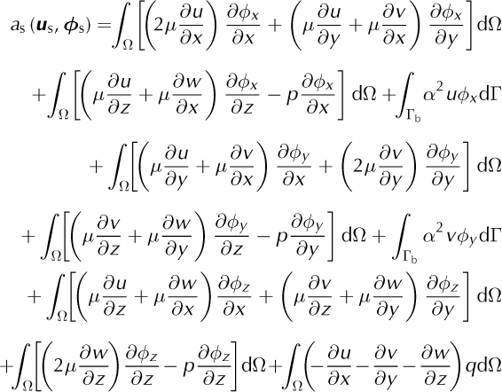

where u s = (u, v, w, p)T and ϕ s = (ϕx, ϕy, ϕz, q)T.
Higher-order model variational formulation
The higher-order model is based on the equations developed by Blatter (1995) and Reference PattynPattyn (2003):

Where s is the upper surface elevation. For this model we use the boundary conditions:

Where n is the outward-pointing normal vector, ρ the ice density, ρ w the water density, (u, v) the horizontal velocity components, τb the tangential components of external forces, v b the tangential velocity at the ice/bedrock interface and α a friction coefficient. The ice pressure is taken equal to the lithostatic pressure.
Let V p be the space of kinematically admissible fields and Γu the part of the border, ∂Ω, where Dirichlet conditions are applied:

The variation formulation for the higher-order model is:
With:
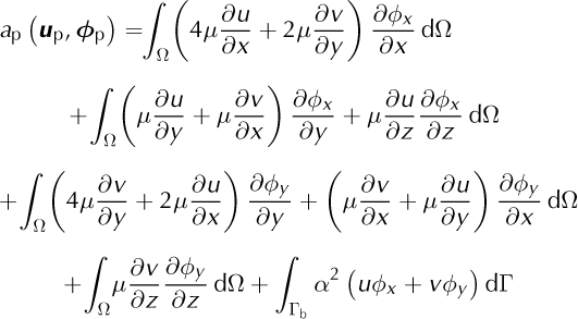

Where u p = (u, v)T , ϕ p = (ϕx, ϕy )T, ρw is water pressure applied at the ice/water interface Γw, Γb the ice/bedrock interface and (n x, n y) the outward pointing normal components.
Shelfy-stream approximation variational formulation
The shelfy-stream approximation is based on the equations developed by MacAyeal (1989) set in Ω:
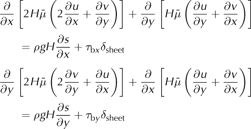
where s is the upper surface elevation and δsheet a function equal to 1 on the ice sheet and 0 on the ice shelf and τb = (τbx, τby) the tangential components of external forces at the ice/bedrock interface. We use the following boundary conditions for the shelfy-stream approximation:

Where n is the outward-pointing normal vector, ρ the ice density, ρ w the water density, H the ice thickness, b the ice lower surface elevation, (u, v) the horizontal velocity components, γi the mean section of the ice front and γu the mean section where Dirichlet conditions are applied. The boundary condition at the ice front is depth-integrated.
Let V m be the space of kinematically admissible velocity fields and Γu the part of the border, ∂Ω, where Dirichlet conditions are applied:

The variation formulation for the shelfy-streem approximation is:

With:


Where u m = (u, v)T, ϕ m = (ϕx, ϕy )T, ρ w is deapth-integrated water pressure applied at the ice front γi and (nx, ny ) the outward-pointing normal components.
Hybrid shelfy-stream/higher-order formulation
The elements outside the blending zone are not affected by the coupling, contrary to the elements in the blending zone, Ωt, because the coupling terms are equal to zero outside the blending zone. The bilinear forms associated with the coupling terms that must be added within the blending zone are

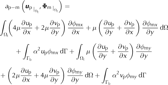
With (u m, v m) the horizontal components of the shelfy-stream velocity, (u p, v p) those of the higher-order model, (ϕ mx, ϕ my) the components of the shelfy-stream admissible velocity field, ϕ m, and (ϕ px , ϕ py ) those of the higher-order admissible velocity field, ϕ p.
Hybrid higher-order/full-Stokes formulation
The terms ![]()
 in Eqn (27) are the usual terms of HO and FS formulations. The other terms are additional terms due to the coupling of the two models. In the previous equation,
 ![]() and
and ![]()
These terms are:

If we write (ϕx, ϕy
) the components of ![]()
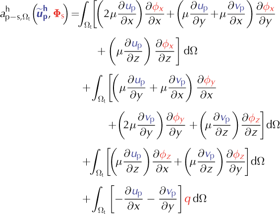
If we write (ϕx, ϕy, ϕz, q) the components of Φ s.

If we write (ϕx, ϕy, ϕz, q) the components of Φ s.


