


1 Introduction
Hughes (Reference Hughes2000) introduced the notion of arrow as an extension of the notion of monad for Haskell to capture non-monadic computational effects. As a syntactic development, the arrow calculus was introduced by Lindley et al. (Reference Lindley, Wadler and Yallop2010). Their calculus is an arrow version of Moggi’s metalanguage (Moggi, Reference Moggi1991). As a semantic development, Heunen and Jacobs (Reference Heunen and Jacobs2006), Jacobs et al. (Reference Jacobs, Heunen and Hasuo2009), Asada (Reference Asada2010) revealed that arrows are strong monads in the bicategory
 $\mathbf{Prof}$
of categories and profunctors.
$\mathbf{Prof}$
of categories and profunctors.
It is a natural question whether we can construct an arrow version of algebraic effects and effect handlers since arrows are an extension of monads. Plotkin and Power (Reference Plotkin and Power2001 a,b) presented an algebraic view for computational effects. Plotkin and Pretnar (Reference Plotkin and Pretnar2013) provided effect handlers as a way to implement effects. Algebraic effects and effect handlers are the foundations of programming languages with effects that correspond to finitary (or more generally ranked) monads. Can we obtain an arrow version of such foundations?
Lindley (Reference Lindley2014) defined an effect system
 $\lambda_{\mathrm{flow}}$
which has algebraic effects and handlers for arrows, monads and idioms. However, the effect system
$\lambda_{\mathrm{flow}}$
which has algebraic effects and handlers for arrows, monads and idioms. However, the effect system
 $\lambda_{\mathrm{flow}}$
is not satisfactory for the following reasons.
$\lambda_{\mathrm{flow}}$
is not satisfactory for the following reasons.
-
• The theoretical background of algebraic effects for arrows is ambiguous. Any categorical explanation of algebraic theories for arrows is not given.
-
• The syntax is complicated. It is unclear why the construction of handlers is given in that way.
-
• Denotational semantics is not defined. It seems hard to give denotational semantics because the algebraic foundation of effects and handlers is not discussed enough.
We present an arrow calculus with operations and handlers as an extension of the arrow calculus. We discuss a categorical foundation for algebraic theories for arrows and give denotational semantics for our calculus by constructing an appropriate strong monad in (![]() )
)![]() . As a main result, soundness and adequacy theorems of the operational semantics with respect to denotational semantics are proven.
. As a main result, soundness and adequacy theorems of the operational semantics with respect to denotational semantics are proven.
Our contributions are as follows.
-
We describe algebras for arrows from a 2-categorical point of view.
-
We present an arrow calculus with operations and handlers based on the notions of algebras for arrows. The progress and preservation theorems for the calculus are shown.
-
We give a denotational semantics for the calculus and prove the soundness theorem.
There are the following non-trivial points in defining the denotational semantics.
-
– The “smallness” of an appropriate strong monad in (
 )
$\mathbf{Prof}$
. The collection of arrow terms, which are arrow analogues of terms in ordinary algebraic theories, is a proper class, not a set. Hence, the “smallness” of a monad that we construct is not trivial. We prove the “smallness” of the monad by counting the number of normal forms of arrow terms, which was introduced by Yallop (Reference Yallop2010) for Haskell programs of arrow types.
)
$\mathbf{Prof}$
. The collection of arrow terms, which are arrow analogues of terms in ordinary algebraic theories, is a proper class, not a set. Hence, the “smallness” of a monad that we construct is not trivial. We prove the “smallness” of the monad by counting the number of normal forms of arrow terms, which was introduced by Yallop (Reference Yallop2010) for Haskell programs of arrow types. -
– A treatment of strength to construct an algebra from a handler. Unlike ordinary handlers, we need a trick to define an interpretation of handlers for arrows because of the strength of strong monads in
$\mathbf{Prof}$
. We define interpretation
$\mathord{\left[\![{{-}}\right]\!]}^{S}$
with a set S as a parameter to construct an algebra from a handler.
-


1.1 Arrows in Haskell
Hughes (Reference Hughes2000, Reference Hughes2005) introduced arrows as a generalisation of monads. In Haskell, arrows are defined using a type class.
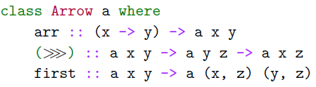
An instance of
 $\mathtt{Arrow}$
is required to satisfy the following arrow laws.
$\mathtt{Arrow}$
is required to satisfy the following arrow laws.
 \begin{align}(a \mathrel{\gt\!\!\gt\!\!\gt} b) \mathrel{\gt\!\!\gt\!\!\gt} c = a \mathrel{\gt\!\!\gt\!\!\gt} (b \mathrel{\gt\!\!\gt\!\!\gt} c)\end{align}
 \begin{align}\mathtt{arr}\ (g \circ f) & = \mathtt{arr}\ f \mathrel{\gt\!\!\gt\!\!\gt} \mathtt{arr}\ g\end{align}
 \begin{align}\mathtt{arr}\ \mathrm{id} \mathrel{\gt\!\!\gt\!\!\gt} a & = a\end{align}
 \begin{align}a \mathrel{\gt\!\!\gt\!\!\gt} \mathtt{arr}\ \mathrm{id} & = a\end{align}
 \begin{align}\mathtt{first}\ a \mathrel{\gt\!\!\gt\!\!\gt} \mathtt{arr}\ (\mathrm{id} \times f) & = \mathtt{arr}\ (\mathrm{id} \times f) \mathrel{\gt\!\!\gt\!\!\gt} \mathtt{first}\ a\end{align}
 \begin{align}\mathtt{first}\ a \mathrel{\gt\!\!\gt\!\!\gt} \mathtt{arr}\ \pi_1 & = \mathtt{arr}\ \pi_1 \mathrel{\gt\!\!\gt\!\!\gt} a\end{align}
 \begin{align}\mathtt{first}\ a \mathrel{\gt\!\!\gt\!\!\gt} \mathtt{arr}\ \alpha & = \mathtt{arr}\ \alpha \mathrel{\gt\!\!\gt\!\!\gt} \mathtt{first}\ (\mathtt{first}\ a)\end{align}
 \begin{align}\mathtt{first}\ (\mathtt{arr}\ f) & = \mathtt{arr}\ (f \times \mathrm{id})\end{align}
 \begin{align}\mathtt{first}\ (a \mathrel{\gt\!\!\gt\!\!\gt} b) & = \mathtt{first}\ a \mathrel{\gt\!\!\gt\!\!\gt} \mathtt{first}\ b\end{align}
where
 $\pi_1 \colon X \times Y \to X$
is a projection, and
$\pi_1 \colon X \times Y \to X$
is a projection, and
 $\alpha \colon (X \times Y) \times Z \to X \times (Y \times Z)$
is an associator.
$\alpha \colon (X \times Y) \times Z \to X \times (Y \times Z)$
is an associator.
We explain some intuition of the type class
 $\mathtt{Arrow}$
. Let
$\mathtt{Arrow}$
. Let
 $\mathtt{A}$
be an instance of
$\mathtt{A}$
be an instance of
 $\mathtt{Arrow}$
. A type
$\mathtt{Arrow}$
. A type
 $\mathtt{A\ x\ y}$
is the type of computations whose input type is
$\mathtt{A\ x\ y}$
is the type of computations whose input type is
 $\mathtt{x}$
and output type is
$\mathtt{x}$
and output type is
 $\mathtt{y}$
. The function
$\mathtt{y}$
. The function
 $\mathtt{arr}$
makes pure computation
$\mathtt{arr}$
makes pure computation
 $\mathtt{arr}\ f$
of type
$\mathtt{arr}\ f$
of type
 $\mathtt{A\ x\ y}$
from a function f of type x -> y. The function
$\mathtt{A\ x\ y}$
from a function f of type x -> y. The function
 $\mathtt{(\mathrel{>\!\!>\!\!>})}$
composes two computations f of type
$\mathtt{(\mathrel{>\!\!>\!\!>})}$
composes two computations f of type
 $\mathtt{A\ x\ y}$
and g of type
$\mathtt{A\ x\ y}$
and g of type
 $\mathtt{A\ y\ z}$
and returns a computation
$\mathtt{A\ y\ z}$
and returns a computation
 $f \mathrel{>\!\!>\!\!>} g$
of type
$f \mathrel{>\!\!>\!\!>} g$
of type
 $\mathtt{A\ x\ z}$
. The function
$\mathtt{A\ x\ z}$
. The function
 $\mathtt{first}$
introduces an additional type z to the input and output types of a computation f of type
$\mathtt{first}$
introduces an additional type z to the input and output types of a computation f of type
 $\mathtt{A\ x\ y}$
and returns a computation
$\mathtt{A\ x\ y}$
and returns a computation
 $\mathtt{first}\ f$
of type
$\mathtt{first}\ f$
of type
 $\mathtt{A\ (x,\ z)\ (y,\ z)}$
.
$\mathtt{A\ (x,\ z)\ (y,\ z)}$
.
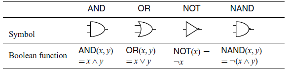
1.2 An example: logic circuit simulation by effects and handlers
Suppose we want to write a simulator for logic circuits. Logic circuits are composed of wires and gates. Wires connect gates and transmit boolean values. There are different types of gates, such as
 $\mathsf{AND}$
,
$\mathsf{AND}$
,
 $\mathsf{OR}$
,
$\mathsf{OR}$
,
 $\mathsf{NOT}$
and
$\mathsf{NOT}$
and
 $\mathsf{NAND}$
. The gates
$\mathsf{NAND}$
. The gates
 $\mathsf{AND}$
,
$\mathsf{AND}$
,
 $\mathsf{OR}$
and
$\mathsf{OR}$
and
 $\mathsf{NAND}$
take two boolean values as inputs and outputs one boolean value. The gate
$\mathsf{NAND}$
take two boolean values as inputs and outputs one boolean value. The gate
 $\mathsf{NOT}$
takes one boolean value as an input and outputs one boolean value. See Table 1 for the definitions as boolean functions of the gates.
$\mathsf{NOT}$
takes one boolean value as an input and outputs one boolean value. See Table 1 for the definitions as boolean functions of the gates.
Table 1. Logic gates
1.2.1 Logic circuit simulation by ordinary algebraic effects and handlers
We can write a simulator for logic circuits in a language with ordinary algebraic effects and handlers. Let
 ${\Sigma_{\mathrm{LC}}}$
be
${\Sigma_{\mathrm{LC}}}$
be ![]() . The set
. The set
 ${\Sigma_{\mathrm{LC}}}$
is a set of algebraic operations and called a signature. For example,
${\Sigma_{\mathrm{LC}}}$
is a set of algebraic operations and called a signature. For example, ![]() is an operation that takes two boolean values as inputs and outputs one boolean value.
is an operation that takes two boolean values as inputs and outputs one boolean value.
First, we write a handler to implement
 $\mathsf{NAND}$
and
$\mathsf{NAND}$
and
 $\mathsf{OR}$
by
$\mathsf{OR}$
by
 $\mathsf{AND}$
and
$\mathsf{AND}$
and
 $\mathsf{NOT}$
.
$\mathsf{NOT}$
.
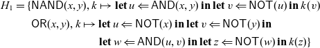 \begin{align*} H_1 = \{ & \mathsf{NAND}(x,y), k \mapsto \mathop{\mathbf{let}} u \Leftarrow \mathsf{AND}(x,y) \mathop{\mathbf{in}} \mathop{\mathbf{let}} v \Leftarrow \mathsf{NOT}(u) \mathop{\mathbf{in}} k(v) \\ & \mathsf{OR}(x,y), k \mapsto \mathop{\mathbf{let}} u \Leftarrow \mathsf{NOT}(x) \mathop{\mathbf{in}} \mathop{\mathbf{let}} v \Leftarrow \mathsf{NOT}(y) \mathop{\mathbf{in}} \\ & \hspace{2cm} \mathop{\mathbf{let}} w \Leftarrow \mathsf{AND}(u,v) \mathop{\mathbf{in}} \mathop{\mathbf{let}} z \Leftarrow \mathsf{NOT}(w) \mathop{\mathbf{in}} k(z) \}\end{align*}
Second, we write a handler to implement
 $\mathsf{NOT}$
and
$\mathsf{NOT}$
and
 $\mathsf{AND}$
.
$\mathsf{AND}$
.
 \begin{align*} H_2 = \{ & \mathsf{AND}(x,y), k \mapsto \mathop{\mathbf{if}} x \mathop{\mathbf{then}} (\mathop{\mathbf{if}} y \mathop{\mathbf{then}} k(\mathtt{true}) \mathop{\mathbf{else}} k(\mathtt{false})) \mathop{\mathbf{else}} k(\mathtt{false}) \\ & \mathsf{NOT}(x), k \mapsto \mathop{\mathbf{if}} x \mathop{\mathbf{then}} k(\mathtt{false}) \mathop{\mathbf{else}} k(\mathtt{true}) \}\end{align*}
By the handlers
 $H_1$
and
$H_1$
and
 $H_2$
, we can simulate logic circuits. For example, we define a program P as
$H_2$
, we can simulate logic circuits. For example, we define a program P as
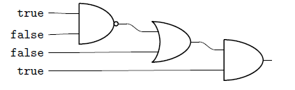
 \begin{equation} P = \left( \mathop{\mathbf{let}} x \Leftarrow \mathsf{NAND}(\mathtt{true}, \mathtt{false}) \mathop{\mathbf{in}} \mathop{\mathbf{let}} y \Leftarrow \mathsf{OR}(x, \mathtt{false}) \mathop{\mathbf{in}} \mathsf{AND}(y, \mathtt{true}) \right).\end{equation}
The program P corresponds to the following logic circuit.
Then, we can obtain the simulation result of P by handling it with
 $H_1$
and
$H_1$
and
 $H_2$
:
$H_2$
:
 \begin{equation*} \mathop{\mathbf{handle}} (\mathop{\mathbf{handle}} P \mathop{\mathbf{with}} H_1) \mathop{\mathbf{with}} H_2 \to^* \mathtt{true}.\end{equation*}
The advantage of using handlers is that the structure of a logic circuit can be separated from its implementation. We can use a different implementation for logic circuits using the following handlers:
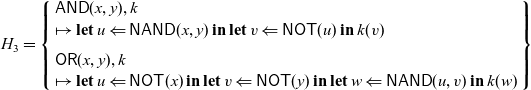 \begin{equation*} H_3 = \left\{ \begin{array}{l} \mathsf{AND}(x,y), k \\ \mapsto \mathop{\mathbf{let}} u \Leftarrow \mathsf{NAND}(x,y) \mathop{\mathbf{in}} \mathop{\mathbf{let}} v \Leftarrow \mathsf{NOT}(u) \mathop{\mathbf{in}} k(v) \\[0.5em] \mathsf{OR}(x,y), k \\ \mapsto \mathop{\mathbf{let}} u \Leftarrow \mathsf{NOT}(x) \mathop{\mathbf{in}} \mathop{\mathbf{let}} v \Leftarrow \mathsf{NOT}(y) \mathop{\mathbf{in}} \mathop{\mathbf{let}} w \Leftarrow \mathsf{NAND}(u,v) \mathop{\mathbf{in}} k(w) \end{array} \right\}\end{equation*}
 \begin{equation*} H_4 = \{ \mathsf{NOT}(x), k \mapsto \mathop{\mathbf{let}} u \Leftarrow \mathsf{NAND}(x,x) \mathop{\mathbf{in}} k(u) \},\end{equation*}
 \begin{equation*} H_5 = \{\mathsf{NAND}(x,y), k \mapsto \mathop{\mathbf{if}} x \mathop{\mathbf{then}} (\mathop{\mathbf{if}} y \mathop{\mathbf{then}} k(\mathtt{false}) \mathop{\mathbf{else}} k(\mathtt{true})) \mathop{\mathbf{else}} k(\mathtt{true}) \}.\end{equation*}
We have
 $\mathop{\mathbf{handle}} (\mathop{\mathbf{handle}} (\mathop{\mathbf{handle}} P \mathop{\mathbf{with}} H_3) \mathop{\mathbf{with}} H_4) \mathop{\mathbf{with}} H_5 \to^* \mathtt{true}$
.
$\mathop{\mathbf{handle}} (\mathop{\mathbf{handle}} (\mathop{\mathbf{handle}} P \mathop{\mathbf{with}} H_3) \mathop{\mathbf{with}} H_4) \mathop{\mathbf{with}} H_5 \to^* \mathtt{true}$
.
1.2.2 A problem of the approach with ordinary effects and handlers
Although we can write logic circuits with ordinary algebraic effects, the expressive power of programming languages with such effects is too high. This is because it is possible to describe dynamic- or meta-operations on circuits that cannot be realised in normal circuits. For example, let Q be the following program:
 \begin{equation} Q = \left( \mathop{\mathbf{let}} x \Leftarrow \mathsf{AND}(\mathtt{true}, \mathtt{false}) \mathop{\mathbf{in}} \mathop{\mathbf{if}} x \mathop{\mathbf{then}} \mathsf{AND}(x, \mathtt{true}) \mathop{\mathbf{else}} \mathsf{NOT}(x) \right).\end{equation}
This program corresponds to the following “logic circuit.”
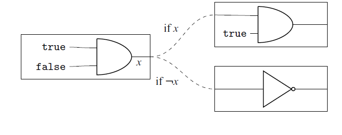
The above “logic circuit” has dynamic selection of circuits according to the output value of the first
 $\mathsf{AND}$
gate. Since such dynamic selection is an “out-of-circuit” operation, we want to restrict the possibility of writing such a program.
$\mathsf{AND}$
gate. Since such dynamic selection is an “out-of-circuit” operation, we want to restrict the possibility of writing such a program.
1.2.3 Logic circuit simulation by the arrow calculus with operations and handlers
Since arrows generalise monads, the expression power of arrows is weaker than that of monads. We can exploit the constraints to restrict dynamic selection of logic circuits. Algebraic effects that correspond to arrows, which we introduce as the arrow calculus with operation and handlers in this paper, have a restriction such that it is impossible to perform conditional branching on their output to select subsequent algebraic effects.
The formal syntax of the arrow calculus with operations and handlers is given in Section 4.1. Here, we give informal descriptions of the syntax and explain the restriction.
The arrow calculus has two kinds of judgements:
where
 $\Gamma = x_1 : A_1, \dots, x_n : A_n$
and
$\Gamma = x_1 : A_1, \dots, x_n : A_n$
and
 $\Delta = y_1 : B_1, \dots, y_m : B_m$
are typing environments and A is a type. The term M is a pure function of the context, of type A. The command P is a computation which takes inputs of types
$\Delta = y_1 : B_1, \dots, y_m : B_m$
are typing environments and A is a type. The term M is a pure function of the context, of type A. The command P is a computation which takes inputs of types
 $\Delta$
and returns an output of type A under the context
$\Delta$
and returns an output of type A under the context
 $\Gamma$
. Compared to the arrow class in Haskell (Section 1.1), the command P corresponds to a Haskell function of type “
$\Gamma$
. Compared to the arrow class in Haskell (Section 1.1), the command P corresponds to a Haskell function of type “
 $\Gamma \to \mathtt{Ar}\ \Delta\ A$
” where
$\Gamma \to \mathtt{Ar}\ \Delta\ A$
” where
 $\mathtt{Ar}$
is an instance of the arrow class
$\mathtt{Ar}$
is an instance of the arrow class
 $\mathtt{Arrow}$
.
$\mathtt{Arrow}$
.
If we have a pure function M from
 $\Delta$
to A, we can obtain a pure command:
$\Delta$
to A, we can obtain a pure command:

This rule corresponds to
 $\mathtt{arr}$
of the class
$\mathtt{arr}$
of the class
 $\mathtt{Arrow}$
in Haskell.
$\mathtt{Arrow}$
in Haskell.
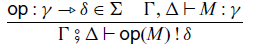
Let
 $\Sigma$
be a set of operations, called a signature. For an operation
$\Sigma$
be a set of operations, called a signature. For an operation
 $\mathsf{op} \in \Sigma$
, we can perform the operation with an input M:
$\mathsf{op} \in \Sigma$
, we can perform the operation with an input M:
Abstraction and application of commands are given by the following rules, respectively:
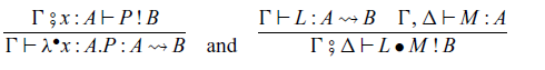
where the type
 $A \rightsquigarrow B$
corresponds to a type
$A \rightsquigarrow B$
corresponds to a type
 $\mathtt{Ar}\ A\ B$
in Haskell. The rule for
$\mathtt{Ar}\ A\ B$
in Haskell. The rule for
 $L \bullet M$
corresponds to
$L \bullet M$
corresponds to
 $\mathtt{(\mathrel{>\!\!>\!\!>})}$
of the class
$\mathtt{(\mathrel{>\!\!>\!\!>})}$
of the class
 $\mathtt{Arrow}$
in Haskell.
$\mathtt{Arrow}$
in Haskell.
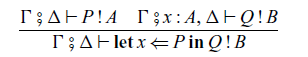
We also have sequential composition
 $\mathop{\mathbf{let}} x \Leftarrow P \mathop{\mathbf{in}} Q$
of commands P and Q, which corresponds to
$\mathop{\mathbf{let}} x \Leftarrow P \mathop{\mathbf{in}} Q$
of commands P and Q, which corresponds to
 $\mathtt{(\mathrel{>\!\!>\!\!>})}$
and
$\mathtt{(\mathrel{>\!\!>\!\!>})}$
and
 $\mathtt{first}$
in Haskell:
$\mathtt{first}$
in Haskell:
For terms M,
 $N_1$
and
$N_1$
and
 $N_2$
, we can add
$N_2$
, we can add
 $\mathop{\mathbf{if}} M \mathop{\mathbf{then}} N_1 \mathop{\mathbf{else}} N_2$
to the arrow calculus. If we add a conditional branching like
$\mathop{\mathbf{if}} M \mathop{\mathbf{then}} N_1 \mathop{\mathbf{else}} N_2$
to the arrow calculus. If we add a conditional branching like
 $\mathop{\mathbf{if}} M \mathop{\mathbf{then}} P_1 \mathop{\mathbf{else}} P_2$
, where
$\mathop{\mathbf{if}} M \mathop{\mathbf{then}} P_1 \mathop{\mathbf{else}} P_2$
, where
 $P_1$
and
$P_1$
and
 $P_2$
are commands, to the syntax of the arrow calculus, we cannot interpret the calculus using strong promonads. This is an important difference from the ordinary algebraic effects.
$P_2$
are commands, to the syntax of the arrow calculus, we cannot interpret the calculus using strong promonads. This is an important difference from the ordinary algebraic effects.
This restriction comes from semantic observation. A term of an algebra of a promonad, which is a semantic counterpart of arrows, is a sequence (without branching) of operations, whereas a term of an algebra of an ordinary monad is a tree of operations. Hence, we cannot add a conditional branching to the arrow calculus because the algebraic structure has no branching, and we can do conditional branching in a language with ordinary algebraic effects because the algebraic structure has branching. This observation is informally described by Lindley (Reference Lindley2014), and we give a formal explanation in Section 5.2.
Let us return to the simulation of logic circuits. Now we can restrict the dynamic selection of circuits by using the constraints of the arrow calculus. The program P defined by (1.10) is also a valid program in the arrow calculus, and Q defined by (1.11) is not a program in the arrow calculus.
In the arrow calculus with operations and handlers, handlers
 $H'_1$
and
$H'_1$
and
 $H'_2$
corresponding to
$H'_2$
corresponding to
 $H_1$
and
$H_1$
and
 $H_2$
are defined as follows.
$H_2$
are defined as follows.
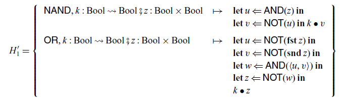
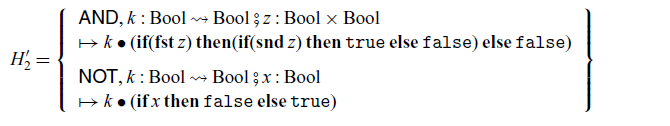
Note that, in the construction of
 $H'_2$
, we can use
$H'_2$
, we can use
 $\mathop{\mathbf{if}}$
’s because these
$\mathop{\mathbf{if}}$
’s because these
 $\mathop{\mathbf{if}}$
’s select terms, not commands.
$\mathop{\mathbf{if}}$
’s select terms, not commands.
We can simulate logic circuits by handling P with
 $H'_1$
and
$H'_1$
and
 $H'_2$
:
$H'_2$
:
 \begin{equation*} \mathop{\mathbf{handle}} (\mathop{\mathbf{handle}} P \mathop{\mathbf{with}} H'_1) \mathop{\mathbf{with}} H'_2 \to^* \lfloor{\mathtt{true}}\rfloor.\end{equation*}
We can also construct handlers
 $H'_3$
,
$H'_3$
,
 $H'_4$
and
$H'_4$
and
 $H'_5$
corresponding to
$H'_5$
corresponding to
 $H_3$
,
$H_3$
,
 $H_4$
and
$H_4$
and
 $H_5$
. For more details, see Section 4.3.1.
$H_5$
. For more details, see Section 4.3.1.
1.3 The structure of this paper
The rest of this paper is organised as follows. Section 2 is a section on categorical preliminaries. In Section 3, we describe algebras for a monad in the bicategory of categories and profunctors and observe the universality of a free algebra. The arrow calculus with operations and handlers is introduced in Section 4. Typing rules and operational semantics are presented. In Section 5, we define the denotational semantics for the arrow calculus with operations and handlers. The definition of models is given in Section 5.1. We tackle the “smallness” problem and construct a model in Section 5.2. In Section 5.3, we define the interpretation with attention to the treatment of strength. Soundness and adequacy are shown in Section 5.4.
2 Preliminaries on category theory
In this paper, we assume that the readers are familiar with basic notions of category theory such as adjunctions, monads, presheaves, the Yoneda lemma, Eilenberg–Moore categories and monoidal categories as described in a textbook by Mac Lane (Reference Mac Lane1971). A textbook by Leinster (Reference Leinster2014) is also a good reference for category theory. We use advanced topics of category theory such as coends, 2-categories, bicategories and enriched categories. Readers unfamiliar with coends are referred to Appendix A. Readers unfamiliar with higher categories such as 2-categories, bicategories and enriched categories are referred to Appendix B.
Throughout this paper, we use the following notation.
Notation 2.1. We denote the categories of sets and maps and classes and maps of classes as
 $\mathbf{Set}$
and
$\mathbf{Set}$
and
 $\mathbf{Ens}$
, respectively. The 2-category of small categories and functors is denoted by
$\mathbf{Ens}$
, respectively. The 2-category of small categories and functors is denoted by
 $\mathbf{Cat}$
. For a category
$\mathbf{Cat}$
. For a category
 $\mathbb{C}$
, we write the class of objects of
$\mathbb{C}$
, we write the class of objects of
 $\mathbb{C}$
as
$\mathbb{C}$
as
 $\mathrm{Ob}(\mathbb{C})$
. We write
$\mathrm{Ob}(\mathbb{C})$
. We write
 $\mathrm{Id}_{\mathbb{C}}$
for the identity functor on
$\mathrm{Id}_{\mathbb{C}}$
for the identity functor on
 $\mathbb{C}$
. When a category
$\mathbb{C}$
. When a category
 $\mathbb{C} = (\mathbb{C}, \otimes, J)$
is symmetric monoidal closed, we write
$\mathbb{C} = (\mathbb{C}, \otimes, J)$
is symmetric monoidal closed, we write
 $\Lambda \colon \mathbb{C}(A \otimes B, C) \to \mathbb{C}(A, B \Rightarrow C)$
for the currying operator, where
$\Lambda \colon \mathbb{C}(A \otimes B, C) \to \mathbb{C}(A, B \Rightarrow C)$
for the currying operator, where
 $B \Rightarrow C$
is an internal hom of the symmetric monoidal closed category
$B \Rightarrow C$
is an internal hom of the symmetric monoidal closed category
 $\mathbb{C}$
.
$\mathbb{C}$
.
2.1 Profunctors
Arrows can be seen as strong monads in the bicategory
 $\mathbf{Prof}$
of categories and profunctors (Heunen and Jacobs, Reference Heunen and Jacobs2006; Jacobs et al., Reference Jacobs, Heunen and Hasuo2009; Asada, Reference Asada2010). We review profunctors and strong monads in
$\mathbf{Prof}$
of categories and profunctors (Heunen and Jacobs, Reference Heunen and Jacobs2006; Jacobs et al., Reference Jacobs, Heunen and Hasuo2009; Asada, Reference Asada2010). We review profunctors and strong monads in
 $\mathbf{Prof}$
.
$\mathbf{Prof}$
.
In the following definition of profunctors, we use coends, which are defined and gave an informal description in Appendix A. For more detailed explanation of coends, see also Mac Lane (Reference Mac Lane1971, Section 9) or Loregian (Reference Loregian2021, Section 1).
Definition 2.2 (profunctor, Bénabou, Reference Bénabou2000). Let
 $\mathbb{C}$
and
$\mathbb{C}$
and
 $\mathbb{D}$
be categories. A profunctor
$\mathbb{D}$
be categories. A profunctor ![]() from
from
 $\mathbb{C}$
to
$\mathbb{C}$
to
 $\mathbb{D}$
is a functor
$\mathbb{D}$
is a functor
 $F \colon \mathbb{D}^{\mathrm{op}} \times \mathbb{C} \to \mathbf{Set}$
. For profunctors
$F \colon \mathbb{D}^{\mathrm{op}} \times \mathbb{C} \to \mathbf{Set}$
. For profunctors ![]() and
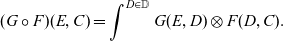
and ![]() , their composite
, their composite ![]() is defined by taking the coend:
is defined by taking the coend:
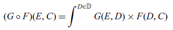 \begin{equation} (G \circ F)(E , C) = \int^{D \in \mathbb{D}} G(E, D) \times F(D, C) \end{equation}
for
 $E \in \mathrm{Ob}(\mathbb{E})$
and
$E \in \mathrm{Ob}(\mathbb{E})$
and
 $C \in \mathrm{Ob}(\mathbb{C})$
. The identity profunctor
$C \in \mathrm{Ob}(\mathbb{C})$
. The identity profunctor ![]() is defined by
is defined by
 \begin{equation*} \mathrm{I}_{\mathbb{C}}(C, D) = \mathbb{C}(C, D) \end{equation*}
for
 $C, D \in \mathrm{Ob}(\mathbb{C})$
. A 2-cell
$C, D \in \mathrm{Ob}(\mathbb{C})$
. A 2-cell
 $\alpha \colon F \Rightarrow G$
between profunctors
$\alpha \colon F \Rightarrow G$
between profunctors ![]() is a natural transformation.
is a natural transformation.
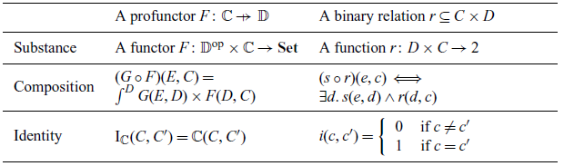
A profunctor ![]() is an analogue of a binary relation
is an analogue of a binary relation
 $r \subseteq C \times D$
between two sets C and D. We identify the binary relation r with its characteristic function
$r \subseteq C \times D$
between two sets C and D. We identify the binary relation r with its characteristic function
 $D \times C \to 2$
. A composition
$D \times C \to 2$
. A composition
 $s \circ r \subseteq C \times E$
of two relations
$s \circ r \subseteq C \times E$
of two relations
 $r \subseteq C \times D$
and
$r \subseteq C \times D$
and
 $s \subseteq D \times E$
is defined as follows:
$s \subseteq D \times E$
is defined as follows:
 \begin{equation*} (s \circ r)(e,c) \iff \exists d \in D.\, s(e, d) \land r(d, c).\end{equation*}
This definition of compositions is similar to the definition of compositions of profunctors (2.1) because the coend operator
 $\int^{D \in \mathbb{D}}({-})$
is an analogue of an existential quantifier
$\int^{D \in \mathbb{D}}({-})$
is an analogue of an existential quantifier
 $\exists D \in \mathbb{D}.\,({-})$
as described in Appendix A. The correspondence between profunctors and binary relations is summarised in Table 2.
$\exists D \in \mathbb{D}.\,({-})$
as described in Appendix A. The correspondence between profunctors and binary relations is summarised in Table 2.
Table 2. Analogy between profunctors and binary relations
A profunctor ![]() is a presheaf
is a presheaf
 $G \colon \mathbb{C}^{\mathrm{op}} \to \mathbf{Set}$
on
$G \colon \mathbb{C}^{\mathrm{op}} \to \mathbf{Set}$
on
 $\mathbb{C}$
. We have
$\mathbb{C}$
. We have
 $(H \circ G) \circ F \cong H \circ (G \circ F)$
and
$(H \circ G) \circ F \cong H \circ (G \circ F)$
and
 $\mathrm{I}_{\mathbb{D}} \circ F \cong F \cong F \circ \mathrm{I}_{\mathbb{C}}$
. That is, associativity and unitality hold up to natural isomorphism, not strictly. Moreover, the class of small categories and profunctors forms a bicategory. Roughly speaking, a bicategory is a “category” whose hom-sets have a category structure and whose composition and identity are associative and unital up to isomorphism. See Appendix B.2 or (1994, Section 7.7) for the definition of bicategories. We write the bicategory of profunctors as
$\mathrm{I}_{\mathbb{D}} \circ F \cong F \cong F \circ \mathrm{I}_{\mathbb{C}}$
. That is, associativity and unitality hold up to natural isomorphism, not strictly. Moreover, the class of small categories and profunctors forms a bicategory. Roughly speaking, a bicategory is a “category” whose hom-sets have a category structure and whose composition and identity are associative and unital up to isomorphism. See Appendix B.2 or (1994, Section 7.7) for the definition of bicategories. We write the bicategory of profunctors as
 $\mathbf{Prof}$
.
$\mathbf{Prof}$
.
From a functor
 $F \colon \mathbb{C} \to \mathbb{D}$
, we can obtain two profunctors
$F \colon \mathbb{C} \to \mathbb{D}$
, we can obtain two profunctors ![]() and
and ![]() which are defined by
which are defined by
 \begin{equation*} {F}_{*}(D, C) = \mathbb{D}(D , FC), \qquad {F}^{*}(C, D) = \mathbb{D}(FC, D)\end{equation*}
on objects
 $C \in \mathrm{Ob}(\mathbb{C})$
and
$C \in \mathrm{Ob}(\mathbb{C})$
and
 $D \in \mathrm{Ob}(\mathbb{D})$
. For morphisms f in
$D \in \mathrm{Ob}(\mathbb{D})$
. For morphisms f in
 $\mathbb{C}$
and g in
$\mathbb{C}$
and g in
 $\mathbb{D}$
,
$\mathbb{D}$
,
 ${F}_{*}(g, f)$
and
${F}_{*}(g, f)$
and
 ${F}^{*}(f, g)$
are also defined appropriately.
${F}^{*}(f, g)$
are also defined appropriately.
2.2 Monads in the bicategory of profunctors
To capture notions of computations, strong monads have been used in functional programming (Moggi, Reference Moggi1989, Reference Moggi1991). In this paper, to capture notions of computation, we use monads in the bicategory
 $\mathbf{Prof}$
instead of ordinary monads, that is monads in the 2-category
$\mathbf{Prof}$
instead of ordinary monads, that is monads in the 2-category
 $\mathbf{Cat}$
. For the definition of monads in 2-categories and bicategories, see Appendices B.1 and B.2.
$\mathbf{Cat}$
. For the definition of monads in 2-categories and bicategories, see Appendices B.1 and B.2.
We call a monad in
 $\mathbf{Prof}$
a promonad. A strong promonad is a promonad with a strength.
$\mathbf{Prof}$
a promonad. A strong promonad is a promonad with a strength.
Definition 2.3. (strong promonad, Asada, Reference Asada2010; Asada and Hasuo, Reference Asada and Hasuo2010). Let
 $\mathbb{C} = (\mathbb{C}, \otimes, J)$
be a monoidal category. A strong promonad on
$\mathbb{C} = (\mathbb{C}, \otimes, J)$
be a monoidal category. A strong promonad on
 $\mathbb{C}$
is a profunctor
$\mathbb{C}$
is a profunctor ![]() with 2-cells
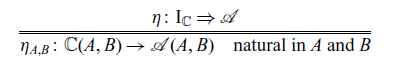
with 2-cells
 $\eta^{\mathcal{A}} \colon \mathrm{I}_{\mathbb{C}} \Rightarrow \mathcal{A}$
,
$\eta^{\mathcal{A}} \colon \mathrm{I}_{\mathbb{C}} \Rightarrow \mathcal{A}$
,
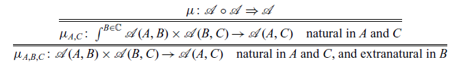
 $\mu^{\mathcal{A}} \colon \mathcal{A} \circ \mathcal{A} \Rightarrow \mathcal{A}$
, and
$\mu^{\mathcal{A}} \colon \mathcal{A} \circ \mathcal{A} \Rightarrow \mathcal{A}$
, and
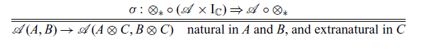
 $\sigma^{\mathcal{A}} \colon ({\otimes}_{*}) \circ (\mathcal{A} \times \mathrm{I}_{\mathbb{C}}) \Rightarrow \mathcal{A} \circ ({\otimes}_{*})$
:
$\sigma^{\mathcal{A}} \colon ({\otimes}_{*}) \circ (\mathcal{A} \times \mathrm{I}_{\mathbb{C}}) \Rightarrow \mathcal{A} \circ ({\otimes}_{*})$
:
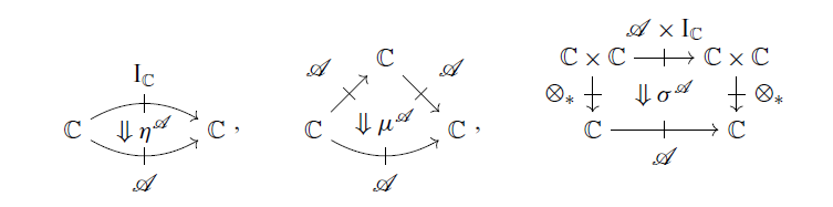
satisfying the axioms shown in Figure 1.
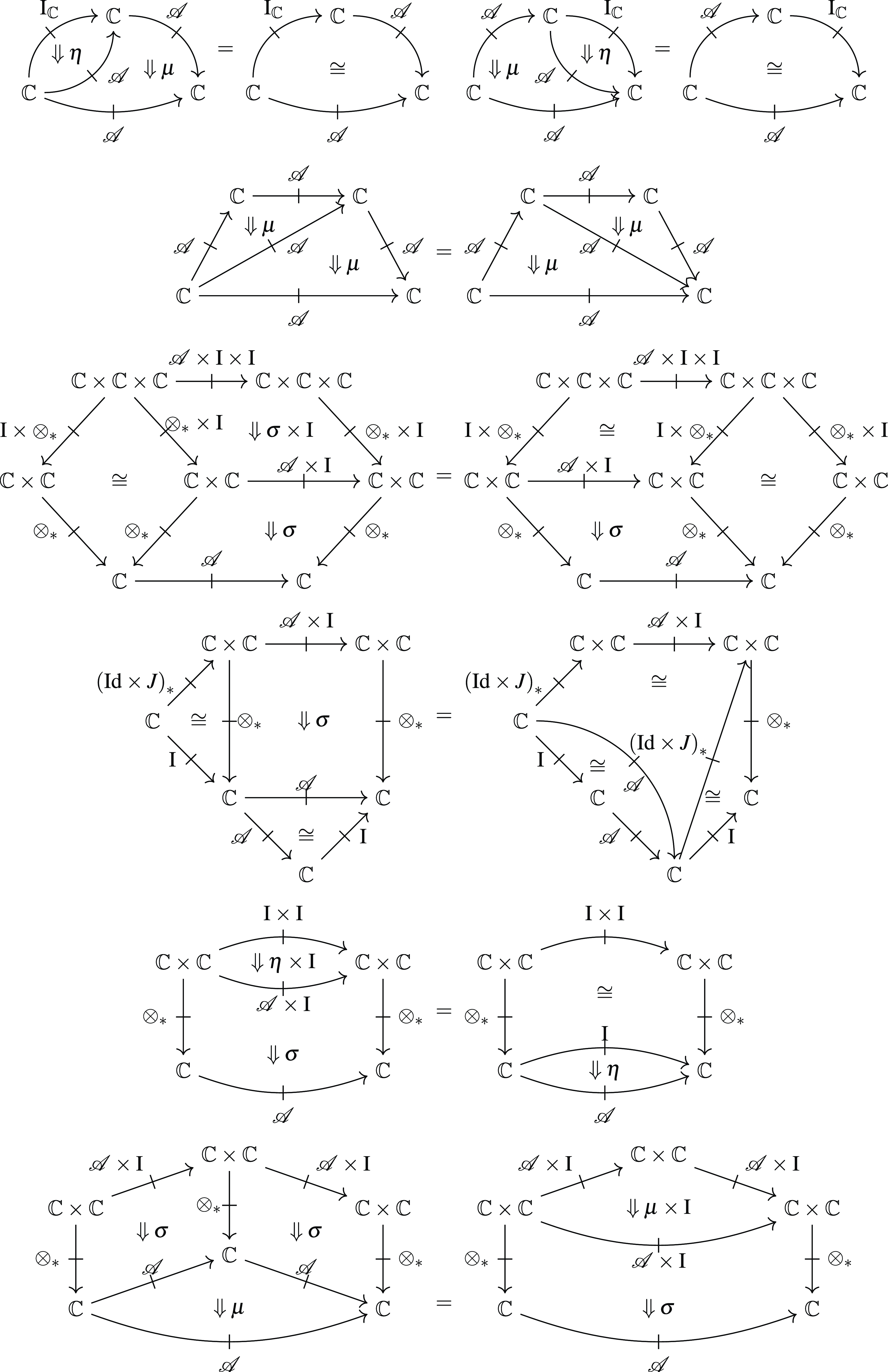
Fig. 1. Axioms for a strong promonad.
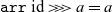
Hughes (Reference Hughes2000), Jacobs et al. (Reference Jacobs, Heunen and Hasuo2009), Asada (Reference Asada2010) showed that a promonad corresponds to an arrow type in Haskell. The unit
 $\eta \colon \mathrm{I}_{\mathbb{C}} \Rightarrow \mathcal{A}$
of a promonad
$\eta \colon \mathrm{I}_{\mathbb{C}} \Rightarrow \mathcal{A}$
of a promonad
 $\mathcal{A}$
corresponds to
$\mathcal{A}$
corresponds to
 $\mathtt{arr}$
: (x -> y) -> A x y:
$\mathtt{arr}$
: (x -> y) -> A x y:
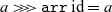
The multiplication
 $\mu \colon \mathcal{A} \circ \mathcal{A} \Rightarrow \mathcal{A}$
of the promonad
$\mu \colon \mathcal{A} \circ \mathcal{A} \Rightarrow \mathcal{A}$
of the promonad
 $\mathcal{A}$
corresponds to
$\mathcal{A}$
corresponds to
 $\mathtt{(\mathrel{>\!\!>\!\!>})}$
: A x y -> A y z -> A x z:
$\mathtt{(\mathrel{>\!\!>\!\!>})}$
: A x y -> A y z -> A x z:
The strength ![]() of the promonad
of the promonad
 $\mathcal{A}$
corresponds to
$\mathcal{A}$
corresponds to
 $\mathtt{first}$
: A x y -> A (x, z) (y, z). The proof of the correspondence is complicated, see Asada (Reference Asada2010, Theorem 14):
$\mathtt{first}$
: A x y -> A (x, z) (y, z). The proof of the correspondence is complicated, see Asada (Reference Asada2010, Theorem 14):
From a monad, we can obtain a promonad:
Proposition 2.4. Let
 $\mathcal{T} \colon \mathbb{C} \to \mathbb{C}$
be a monad. The profunctor
$\mathcal{T} \colon \mathbb{C} \to \mathbb{C}$
be a monad. The profunctor ![]() is a promonad.
is a promonad.
Note that the profunctor ![]() is a functor
is a functor
 $\mathbb{C}^{\mathrm{op}} \times \mathbb{C} \to \mathbf{Set}$
, and we have
$\mathbb{C}^{\mathrm{op}} \times \mathbb{C} \to \mathbf{Set}$
, and we have
 ${\mathcal{T}}_{*}(C, D) = \mathbb{C}(C, \mathcal{T} D) = \mathop{\mathcal{K}\!\!\ell}(\mathcal{T})(C, D)$
where
${\mathcal{T}}_{*}(C, D) = \mathbb{C}(C, \mathcal{T} D) = \mathop{\mathcal{K}\!\!\ell}(\mathcal{T})(C, D)$
where
 $\mathop{\mathcal{K}\!\!\ell}(\mathcal{T})$
is the Kleisli category for the monad
$\mathop{\mathcal{K}\!\!\ell}(\mathcal{T})$
is the Kleisli category for the monad
 $\mathcal{T}$
. Hence, each monad can be regarded as a promonad. In this sense, arrows are a generalisation of monads.
$\mathcal{T}$
. Hence, each monad can be regarded as a promonad. In this sense, arrows are a generalisation of monads.
For a monad
 $\mathcal{T} \colon \mathbb{C} \to \mathbb{C}$
in
$\mathcal{T} \colon \mathbb{C} \to \mathbb{C}$
in
 $\mathbf{Cat}$
, there exists a category
$\mathbf{Cat}$
, there exists a category
 $\mathop{\mathcal{E\!\!M}}(\mathcal{T})$
called the Eilenberg–Moore category of
$\mathop{\mathcal{E\!\!M}}(\mathcal{T})$
called the Eilenberg–Moore category of
 $\mathcal{T}$
. It satisfies the following property (Street, Reference Street1972):
$\mathcal{T}$
. It satisfies the following property (Street, Reference Street1972):
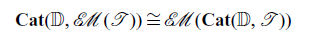 \begin{equation} \mathbf{Cat}(\mathbb{D}, \mathop{\mathcal{E\!\!M}}(\mathcal{T})) \cong \mathop{\mathcal{E\!\!M}}(\mathbf{Cat}(\mathbb{D}, \mathcal{T}))\end{equation}
where
 $\mathbf{Cat}(\mathbb{D}, \mathcal{T}) \colon \mathbf{Cat}(\mathbb{D}, \mathbb{C}) \to \mathbf{Cat}(\mathbb{D}, \mathbb{C})$
on the right-hand side is a monad on the functor category
$\mathbf{Cat}(\mathbb{D}, \mathcal{T}) \colon \mathbf{Cat}(\mathbb{D}, \mathbb{C}) \to \mathbf{Cat}(\mathbb{D}, \mathbb{C})$
on the right-hand side is a monad on the functor category
 $\mathbf{Cat}(\mathbb{D}, \mathbb{C})$
defined by
$\mathbf{Cat}(\mathbb{D}, \mathbb{C})$
defined by
 $\mathbf{Cat}(\mathbb{D}, \mathcal{T})(F) = \mathcal{T} \circ F$
. The category
$\mathbf{Cat}(\mathbb{D}, \mathcal{T})(F) = \mathcal{T} \circ F$
. The category
 $\mathop{\mathcal{E\!\!M}}(\mathbf{Cat}(\mathbb{D}, \mathcal{T}))$
is the Eilenberg–Moore category of the monad
$\mathop{\mathcal{E\!\!M}}(\mathbf{Cat}(\mathbb{D}, \mathcal{T}))$
is the Eilenberg–Moore category of the monad
 $\mathbf{Cat}(\mathbb{D}, \mathcal{T})$
.
$\mathbf{Cat}(\mathbb{D}, \mathcal{T})$
.
For a promonad ![]() in
in
 $\mathbf{Prof}$
, there exists a category
$\mathbf{Prof}$
, there exists a category
 $\mathop{\mathcal{E\!\!M}}(\mathcal{A})$
(Wood, Reference Wood1985) that satisfies
$\mathop{\mathcal{E\!\!M}}(\mathcal{A})$
(Wood, Reference Wood1985) that satisfies
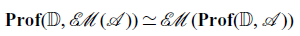 \begin{equation} \mathbf{Prof}(\mathbb{D}, \mathop{\mathcal{E\!\!M}}(\mathcal{A})) \simeq \mathop{\mathcal{E\!\!M}}(\mathbf{Prof}(\mathbb{D}, \mathcal{A}))\end{equation}
where
 $\mathbf{Prof}(\mathbb{D}, \mathcal{A}) \colon \mathbf{Prof}(\mathbb{D}, \mathbb{C}) \to \mathbf{Prof}(\mathbb{D}, \mathbb{C})$
on the right-hand side is a monad on the profunctor category
$\mathbf{Prof}(\mathbb{D}, \mathcal{A}) \colon \mathbf{Prof}(\mathbb{D}, \mathbb{C}) \to \mathbf{Prof}(\mathbb{D}, \mathbb{C})$
on the right-hand side is a monad on the profunctor category
 $\mathbf{Prof}(\mathbb{D}, \mathbb{C})$
defined by
$\mathbf{Prof}(\mathbb{D}, \mathbb{C})$
defined by
 $\mathbf{Prof}(\mathbb{D}, \mathcal{A})(F) = \mathcal{A} \circ F$
.
$\mathbf{Prof}(\mathbb{D}, \mathcal{A})(F) = \mathcal{A} \circ F$
.
Definition 2.5 (the Eilenberg–Moore category of a promonad, Wood, Reference Wood1985). Let ![]() be a promonad in
be a promonad in
 $\mathbf{Prof}$
. The Eilenberg–Moore category
$\mathbf{Prof}$
. The Eilenberg–Moore category
 $\mathop{\mathcal{E\!\!M}}(\mathcal{A})$
of
$\mathop{\mathcal{E\!\!M}}(\mathcal{A})$
of
 $\mathcal{A}$
is defined as follows:
$\mathcal{A}$
is defined as follows:
-
•
$\mathrm{Ob}(\mathop{\mathcal{E\!\!M}}(\mathcal{A})) = \mathrm{Ob}(\mathbb{C})$
. -
• For
$A, B \in \mathrm{Ob}(\mathop{\mathcal{E\!\!M}}(\mathcal{A}))$
,
$\mathop{\mathcal{E\!\!M}}(\mathcal{A})(A, B) = \mathcal{A}(A, B)$
. -
• For
$A \in \mathrm{Ob}(\mathop{\mathcal{E\!\!M}}(\mathcal{A}))$
, the identity on A is
$\eta^{\mathcal{A}}_{A,A}(\mathrm{id}_A) \in \mathcal{A}(A, A)$
. -
• For
$a \in \mathop{\mathcal{E\!\!M}}(\mathcal{A})(A, B)$
and
$b \in \mathop{\mathcal{E\!\!M}}(\mathcal{A})(B, C)$
, the composition
$b \circ a$
is
$\mu^{\mathcal{A}}_{A, B, C}(a, b)$
.


There is an identity-on-objects functor
 $J \colon \mathbb{C} \to \mathop{\mathcal{E\!\!M}}(\mathcal{A})$
defined by
$J \colon \mathbb{C} \to \mathop{\mathcal{E\!\!M}}(\mathcal{A})$
defined by
 $\eta^{\mathcal{A}}_{A, B} \colon \mathbb{C}(A, B) \to \mathcal{A}(A, B)$
. The functor J induces an adjunction
$\eta^{\mathcal{A}}_{A, B} \colon \mathbb{C}(A, B) \to \mathcal{A}(A, B)$
. The functor J induces an adjunction
 ${J}_{*} \dashv {J}^{*}$
in
${J}_{*} \dashv {J}^{*}$
in
 $\mathbf{Prof}$
:
$\mathbf{Prof}$
:
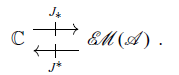
The promonad
 $\mathcal{A}$
coincides with the composition of
$\mathcal{A}$
coincides with the composition of
 ${J}_{*}$
and
${J}_{*}$
and
 ${J}^{*}$
i.e.,
${J}^{*}$
i.e.,
 $\mathcal{A} \cong {J}^{*} \circ {J}_{*}$
.
$\mathcal{A} \cong {J}^{*} \circ {J}_{*}$
.
2.3 Size issues
An arrow corresponds to a strong promonad, but when trying to interpret a programming language with, for example,
 $\mathbf{Set}$
, one faces size problems because the natural interpretation is not a set. That is, an endoprofunctor
$\mathbf{Set}$
, one faces size problems because the natural interpretation is not a set. That is, an endoprofunctor ![]() must be a functor
must be a functor
 $\mathcal{A} \colon \mathbf{Set}^{\mathrm{op}} \times \mathbf{Set} \to \mathbf{Ens}$
, not a functor
$\mathcal{A} \colon \mathbf{Set}^{\mathrm{op}} \times \mathbf{Set} \to \mathbf{Ens}$
, not a functor
 $\mathbf{Set}^{\mathrm{op}} \times \mathbf{Set} \to \mathbf{Set}$
, because the composition of profunctors is defined by a coend. Hence, the interpretation
$\mathbf{Set}^{\mathrm{op}} \times \mathbf{Set} \to \mathbf{Set}$
, because the composition of profunctors is defined by a coend. Hence, the interpretation
 $\mathcal{A}(\mathord{\left[\![{A}\right]\!]}, \mathord{\left[\![{B}\right]\!]})$
of an arrow type
$\mathcal{A}(\mathord{\left[\![{A}\right]\!]}, \mathord{\left[\![{B}\right]\!]})$
of an arrow type
 $A \rightsquigarrow B$
(in a Haskell-like notation,
$A \rightsquigarrow B$
(in a Haskell-like notation,
 $\mathtt{Ar}\ A\ B$
, where
$\mathtt{Ar}\ A\ B$
, where
 $\mathtt{Ar}$
is an instance of the class
$\mathtt{Ar}$
is an instance of the class
 $\mathtt{Arrow}$
) is a class, not a set. Asada (Reference Asada2010) introduced
$\mathtt{Arrow}$
) is a class, not a set. Asada (Reference Asada2010) introduced
 $\mathbb{V}$
-small profunctors in
$\mathbb{V}$
-small profunctors in ![]() . The size problem is solved using
. The size problem is solved using
 $\mathbf{Set}$
-small profunctors in
$\mathbf{Set}$
-small profunctors in ![]() .
.
Readers who are not concerned about size issues may skip the rest of this section. For the definition of enriched categorical notions such as
 $\mathbb{V}$
-categories and
$\mathbb{V}$
-categories and
 $\mathbb{V}$
-functors, see Appendix B.3 and Kelly (Reference Kelly1982, Section 1).
$\mathbb{V}$
-functors, see Appendix B.3 and Kelly (Reference Kelly1982, Section 1).
Definition 2.6 (
 $\mathbb{V}$
-profunctors). Let
$\mathbb{V}$
-profunctors). Let
 $\mathbb{V}$
be a sufficiently cocomplete symmetric monoidal category and
$\mathbb{V}$
be a sufficiently cocomplete symmetric monoidal category and
 $\mathbb{C}$
and
$\mathbb{C}$
and
 $\mathbb{D}$
be
$\mathbb{D}$
be
 $\mathbb{V}$
-categories. A
$\mathbb{V}$
-categories. A
 $\mathbb{V}$
-profunctor F from
$\mathbb{V}$
-profunctor F from
 $\mathbb{C}$
to
$\mathbb{C}$
to
 $\mathbb{D}$
, written
$\mathbb{D}$
, written ![]() , is a
, is a
 $\mathbb{V}$
-functor
$\mathbb{V}$
-functor
 $F \colon \mathbb{D}^{\mathrm{op}} \otimes \mathbb{C} \to \mathbb{V}$
. A 2-cell
$F \colon \mathbb{D}^{\mathrm{op}} \otimes \mathbb{C} \to \mathbb{V}$
. A 2-cell
 $\alpha$
from
$\alpha$
from
 $\mathbb{V}$
-profunctors
$\mathbb{V}$
-profunctors ![]() to
to ![]() , written
, written
 $\alpha \colon F \Rightarrow G$
is a
$\alpha \colon F \Rightarrow G$
is a
 $\mathbb{V}$
-natural transformation between the
$\mathbb{V}$
-natural transformation between the
 $\mathbb{V}$
-functors. For two
$\mathbb{V}$
-functors. For two
 $\mathbb{V}$
-profunctors
$\mathbb{V}$
-profunctors ![]() and
and ![]() , their composite
, their composite ![]() is defined by the following coend in
is defined by the following coend in
 $\mathbb{V}$
:
$\mathbb{V}$
:
 \begin{equation*} (G \circ F)(E, C) = \int^{D \in \mathbb{D}} G(E, D) \otimes F(D, C). \end{equation*}
The identity
 $\mathbb{V}$
-profunctor
$\mathbb{V}$
-profunctor ![]() is defined by
is defined by
 \begin{equation*} \mathrm{I}_{\mathbb{C}}(C, D) = \mathbb{C}(C, D). \end{equation*}
The collection of small
 $\mathbb{V}$
-categories,
$\mathbb{V}$
-categories,
 $\mathbb{V}$
-profunctors and 2-cells, forms a bicategory
$\mathbb{V}$
-profunctors and 2-cells, forms a bicategory ![]() . The bicategory
. The bicategory
 $\mathbf{Prof}$
is the special case of
$\mathbf{Prof}$
is the special case of ![]() where
where
 $\mathbb{V} = (\mathbf{Set}, \times, 1)$
.
$\mathbb{V} = (\mathbf{Set}, \times, 1)$
.
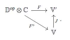
Definition 2.7 (Asada, Reference Asada2010). Let
 $\mathbb{V}$
be a symmetric monoidal category,
$\mathbb{V}$
be a symmetric monoidal category,
 $\mathbb{V}'$
be a sufficiently cocomplete symmetric monoidal closed category and
$\mathbb{V}'$
be a sufficiently cocomplete symmetric monoidal closed category and
 $J \colon \mathbb{V} \to \mathbb{V}'$
be a symmetric strong monoidal fully faithful functor. A
$J \colon \mathbb{V} \to \mathbb{V}'$
be a symmetric strong monoidal fully faithful functor. A
 $\mathbb{V}'$
-profunctor
$\mathbb{V}'$
-profunctor ![]() is
is
 $\mathbb{V}$
-small if there exists a
$\mathbb{V}$
-small if there exists a
 $\mathbb{V}'$
-functor
$\mathbb{V}'$
-functor
 $F^{\circ} \colon \mathbb{D}^{\mathrm{op}} \otimes \mathbb{C} \to \mathbb{V}$
such that
$F^{\circ} \colon \mathbb{D}^{\mathrm{op}} \otimes \mathbb{C} \to \mathbb{V}$
such that
 $J \circ F^{\circ} = F$
:
$J \circ F^{\circ} = F$
:
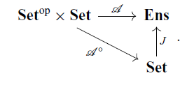
Let
 $J \colon \mathbf{Set} \to \mathbf{Ens}$
be the embedding. A
$J \colon \mathbf{Set} \to \mathbf{Ens}$
be the embedding. A
 $\mathbf{Set}$
-small strong
$\mathbf{Set}$
-small strong
 $\mathbf{Ens}$
-promonad
$\mathbf{Ens}$
-promonad ![]() is an
is an
 $\mathbf{Ens}$
-functor
$\mathbf{Ens}$
-functor
 $\mathcal{A} \colon \mathbf{Set}^{\mathrm{op}} \times \mathbf{Set} \to \mathbf{Ens}$
with 2-cells
$\mathcal{A} \colon \mathbf{Set}^{\mathrm{op}} \times \mathbf{Set} \to \mathbf{Ens}$
with 2-cells
 $\eta$
,
$\eta$
,
 $\mu$
and
$\mu$
and
 $\sigma$
which make
$\sigma$
which make
 $\mathcal{A}$
a strong
$\mathcal{A}$
a strong
 $\mathbf{Ens}$
-promonad, and an
$\mathbf{Ens}$
-promonad, and an
 $\mathbf{Ens}$
-functor
$\mathbf{Ens}$
-functor
 $\mathcal{A}^{\circ} \colon \mathbf{Set}^{\mathrm{op}} \times \mathbf{Set} \to \mathbf{Set}$
satisfying
$\mathcal{A}^{\circ} \colon \mathbf{Set}^{\mathrm{op}} \times \mathbf{Set} \to \mathbf{Set}$
satisfying
If a suitable
 $\mathbf{Set}$
-small strong
$\mathbf{Set}$
-small strong
 $\mathbf{Ens}$
-promonad
$\mathbf{Ens}$
-promonad ![]() exists, then we can define the interpretation of an arrow type
exists, then we can define the interpretation of an arrow type
 $A \rightsquigarrow B$
(which will be introduced in Section 4.1) by
$A \rightsquigarrow B$
(which will be introduced in Section 4.1) by
 $\mathord{\left[\![{A \rightsquigarrow B}\right]\!]} = \mathcal{A}^{\circ}(\mathord{\left[\![{A}\right]\!]}, \mathord{\left[\![{B}\right]\!]})$
.
$\mathord{\left[\![{A \rightsquigarrow B}\right]\!]} = \mathcal{A}^{\circ}(\mathord{\left[\![{A}\right]\!]}, \mathord{\left[\![{B}\right]\!]})$
.
We will introduce an arrow calculus with operations and handlers in Section 4.1 and define models of the calculus as appropriate small promonads (Definition 5.1). As a concrete model, we will construct a
 $\mathbf{Set}$
-small strong
$\mathbf{Set}$
-small strong
 $\mathbf{Ens}$
-promonad
$\mathbf{Ens}$
-promonad
 $\mathcal{A}$
which has sufficient structure to interpret the arrow calculus in Section 5.2.
$\mathcal{A}$
which has sufficient structure to interpret the arrow calculus in Section 5.2.
3 Algebras of arrows
For an ordinary monad
 $\mathcal{T} \colon \mathbb{C} \to \mathbb{C}$
, a
$\mathcal{T} \colon \mathbb{C} \to \mathbb{C}$
, a
 $\mathcal{T}$
-algebra is a pair
$\mathcal{T}$
-algebra is a pair
 $\langle A , a \rangle$
of an object
$\langle A , a \rangle$
of an object
 $A \in \mathbb{C}$
and a morphism
$A \in \mathbb{C}$
and a morphism
 $a \colon \mathcal{T} A \to A$
in
$a \colon \mathcal{T} A \to A$
in
 $\mathbb{C}$
satisfying appropriate axioms, that is an object of the Eilenberg-Moore category
$\mathbb{C}$
satisfying appropriate axioms, that is an object of the Eilenberg-Moore category
 $\mathop{\mathcal{E\!\!M}}(\mathcal{T})$
. An ordinary effect handler is interpreted as a homomorphism between two
$\mathop{\mathcal{E\!\!M}}(\mathcal{T})$
. An ordinary effect handler is interpreted as a homomorphism between two
 $\mathcal{T}$
-algebras.
$\mathcal{T}$
-algebras.
What is an
 $\mathcal{A}$
-algebra for a promonad
$\mathcal{A}$
-algebra for a promonad ![]() ? We answer this question in the next section (Section 3.1) from a 2-categorical point of view. We also discuss the universality of a free
? We answer this question in the next section (Section 3.1) from a 2-categorical point of view. We also discuss the universality of a free
 $\mathcal{A}$
-algebra in Section 3.2. A handler for arrows is interpreted as a homomorphism between
$\mathcal{A}$
-algebra in Section 3.2. A handler for arrows is interpreted as a homomorphism between
 $\mathcal{A}$
-algebras in the sense of Section 3.1.
$\mathcal{A}$
-algebras in the sense of Section 3.1.
3.1 Algebras of promonads
Let
 $\mathbf{1}$
be the category with a single object and a single morphism (the identity). For a monad
$\mathbf{1}$
be the category with a single object and a single morphism (the identity). For a monad
 $\mathcal{T} \colon \mathbb{C} \to \mathbb{C}$
, a
$\mathcal{T} \colon \mathbb{C} \to \mathbb{C}$
, a
 $\mathcal{T}$
-algebra is a functor
$\mathcal{T}$
-algebra is a functor
 $\mathbf{1} \to \mathop{\mathcal{E\!\!M}}(\mathcal{T})$
in
$\mathbf{1} \to \mathop{\mathcal{E\!\!M}}(\mathcal{T})$
in
 $\mathbf{Cat}$
. Similarly, for a promonad
$\mathbf{Cat}$
. Similarly, for a promonad ![]() , we call a profunctor
, we call a profunctor ![]() in
in
 $\mathbf{Prof}$
an
$\mathbf{Prof}$
an
 $\mathcal{A}$
-algebra where
$\mathcal{A}$
-algebra where
 $\mathop{\mathcal{E\!\!M}}(\mathcal{A})$
is the Eilenberg–Moore category of
$\mathop{\mathcal{E\!\!M}}(\mathcal{A})$
is the Eilenberg–Moore category of
 $\mathcal{A}$
(Definition 2.5).
$\mathcal{A}$
(Definition 2.5).
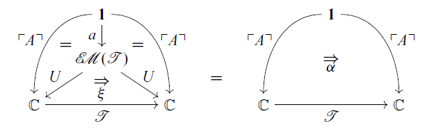
By (2.2), a
 $\mathcal{T}$
-algebra
$\mathcal{T}$
-algebra
 $a \colon \mathbf{1} \to \mathop{\mathcal{E\!\!M}}(\mathcal{T})$
corresponds to a
$a \colon \mathbf{1} \to \mathop{\mathcal{E\!\!M}}(\mathcal{T})$
corresponds to a
 $\mathbf{Cat}(\mathbf{1}, \mathcal{T})$
-algebra
$\mathbf{Cat}(\mathbf{1}, \mathcal{T})$
-algebra
 $\alpha$
, that is the following equation holds:
$\alpha$
, that is the following equation holds:
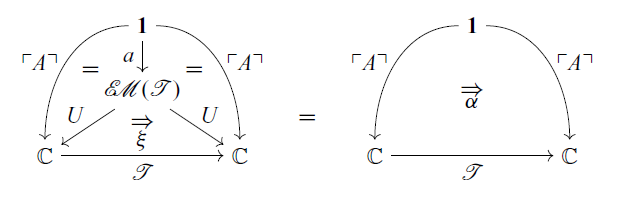
where
 $A \in \mathbb{C}$
,
$A \in \mathbb{C}$
,
 $\ulcorner {A} \urcorner \colon \mathbf{1} \to \mathbb{C}$
is the constant functor, and the 2-cell
$\ulcorner {A} \urcorner \colon \mathbf{1} \to \mathbb{C}$
is the constant functor, and the 2-cell
 $\xi$
is defined by
$\xi$
is defined by
 $\xi_{f} = f \colon \mathcal{T} U (f) \to Uf$
for a
$\xi_{f} = f \colon \mathcal{T} U (f) \to Uf$
for a
 $\mathcal{T}$
-algebra
$\mathcal{T}$
-algebra
 $f \colon \mathcal{T} A \to A$
. Hence, specifying a
$f \colon \mathcal{T} A \to A$
. Hence, specifying a
 $\mathcal{T}$
-algebra
$\mathcal{T}$
-algebra
 $a \colon \mathbf{1} \to \mathop{\mathcal{E\!\!M}}(\mathcal{T})$
is equivalent to specifying a morphism
$a \colon \mathbf{1} \to \mathop{\mathcal{E\!\!M}}(\mathcal{T})$
is equivalent to specifying a morphism
 $\alpha \colon \mathcal{T} A \to A$
satisfying ordinary equations for a
$\alpha \colon \mathcal{T} A \to A$
satisfying ordinary equations for a
 $\mathcal{T}$
-algebra.
$\mathcal{T}$
-algebra.
Similarly, by (2.3), a
 $\mathcal{A}$
-algebra
$\mathcal{A}$
-algebra ![]() corresponds to a
corresponds to a
 $\mathbf{Prof}(\mathbf{1}, \mathcal{A})$
-algebra
$\mathbf{Prof}(\mathbf{1}, \mathcal{A})$
-algebra
 $\alpha$
up to isomorphism, that is
$\alpha$
up to isomorphism, that is
The
 $\mathbf{Prof}(\mathbf{1}, \mathcal{A})$
-algebra
$\mathbf{Prof}(\mathbf{1}, \mathcal{A})$
-algebra
 $\alpha$
satisfies the following equations.
$\alpha$
satisfies the following equations.
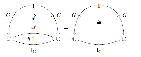
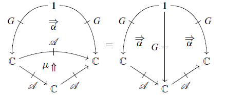
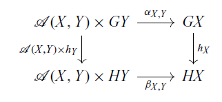
Note that (3.1) is equivalent to
 $\alpha_{X,Y}(\eta_{X,Y}(f), k) = (Gf)(k)$
for any
$\alpha_{X,Y}(\eta_{X,Y}(f), k) = (Gf)(k)$
for any
 $X, Y \in \mathbb{C}$
,
$X, Y \in \mathbb{C}$
,
 $f \in \mathbb{C}(X, Y)$
and
$f \in \mathbb{C}(X, Y)$
and
 $k \in GY$
, and (3.2) is equivalent to
$k \in GY$
, and (3.2) is equivalent to
 $\alpha_{X,Z}(\mu_{X,Y,Z}(a, b), k) = \alpha_{X,Y}(a, \alpha_{Y,Z}(b, k))$
for any
$\alpha_{X,Z}(\mu_{X,Y,Z}(a, b), k) = \alpha_{X,Y}(a, \alpha_{Y,Z}(b, k))$
for any
 $X, Y, Z \in \mathbb{C}$
,
$X, Y, Z \in \mathbb{C}$
,
 $a \in \mathcal{A}(X, Y)$
,
$a \in \mathcal{A}(X, Y)$
,
 $b \in \mathcal{A}(Y, Z)$
and
$b \in \mathcal{A}(Y, Z)$
and
 $k \in GZ$
.
$k \in GZ$
.
Hence, specifying an
 $\mathcal{A}$
-algebra
$\mathcal{A}$
-algebra ![]() is equivalent to specifying a presheaf
is equivalent to specifying a presheaf
 $G \colon \mathbb{C}^{\mathrm{op}} \to \mathbf{Set}$
and a 2-cell
$G \colon \mathbb{C}^{\mathrm{op}} \to \mathbf{Set}$
and a 2-cell
 $\alpha \colon \mathcal{A} \circ G \Rightarrow G$
in
$\alpha \colon \mathcal{A} \circ G \Rightarrow G$
in
 $\mathbf{Prof}$
satisfying (3.1) and (3.2). We call such a pair
$\mathbf{Prof}$
satisfying (3.1) and (3.2). We call such a pair
 $\langle G, \alpha \rangle$
also an algebra.
$\langle G, \alpha \rangle$
also an algebra.
Definition 3.1 (algebras and homomorphisms). Let ![]() be a promonad. An algebra for
be a promonad. An algebra for
 $\mathcal{A}$
is a pair
$\mathcal{A}$
is a pair
 $\langle G, \alpha \rangle$
of a presheaf
$\langle G, \alpha \rangle$
of a presheaf
 $G \colon \mathbb{C}^{\mathrm{op}} \to \mathbf{Set}$
and a 2-cell
$G \colon \mathbb{C}^{\mathrm{op}} \to \mathbf{Set}$
and a 2-cell
 $\alpha \colon \mathcal{A} \circ G \Rightarrow G$
in
$\alpha \colon \mathcal{A} \circ G \Rightarrow G$
in
 $\mathbf{Prof}$
. A homomorphism h from an algebra
$\mathbf{Prof}$
. A homomorphism h from an algebra
 $\langle G, \alpha \rangle$
to an algebra
$\langle G, \alpha \rangle$
to an algebra
 $\langle H, \beta \rangle$
, written
$\langle H, \beta \rangle$
, written
 $h \colon \langle G, \alpha \rangle \to \langle H, \beta \rangle$
, is a 2-cell
$h \colon \langle G, \alpha \rangle \to \langle H, \beta \rangle$
, is a 2-cell
 $h \colon G \Rightarrow H$
in
$h \colon G \Rightarrow H$
in
 $\mathbf{Prof}$
such that
$\mathbf{Prof}$
such that
 $\beta \circ (\mathcal{A} h) = h \circ \alpha$
.
$\beta \circ (\mathcal{A} h) = h \circ \alpha$
.
In other words, a homomorphism
 $h \colon \langle G, \alpha \rangle \to \langle H, \beta \rangle$
is a natural transformation from G to H that makes the following diagram commute:
$h \colon \langle G, \alpha \rangle \to \langle H, \beta \rangle$
is a natural transformation from G to H that makes the following diagram commute:
for any
 $X, Y \in \mathbb{C}$
.
$X, Y \in \mathbb{C}$
.
Remark 3.2. We defined an algebra as a morphism from
 $\mathbf{1}$
to an Eilenberg–Moore object. We justify the use of
$\mathbf{1}$
to an Eilenberg–Moore object. We justify the use of
 $\mathbf{1}$
. A morphism
$\mathbf{1}$
. A morphism
 $\mathbb{D} \to \mathop{\mathcal{E\!\!M}}(\mathcal{T})$
in
$\mathbb{D} \to \mathop{\mathcal{E\!\!M}}(\mathcal{T})$
in
 $\mathbf{Cat}$
corresponds to
$\mathbf{Cat}$
corresponds to
 $\mathbf{1} \to \mathop{\mathcal{E\!\!M}}(\mathbf{Cat}(\mathbb{D}, \mathcal{T}))$
. Similarly, a morphism
$\mathbf{1} \to \mathop{\mathcal{E\!\!M}}(\mathbf{Cat}(\mathbb{D}, \mathcal{T}))$
. Similarly, a morphism ![]() in
in
 $\mathbf{Prof}$
corresponds to
$\mathbf{Prof}$
corresponds to ![]() . In both case, a morphism from a category
. In both case, a morphism from a category
 $\mathbb{D}$
to an Eilenberg–Moore object of a (pro)monad corresponds to a morphism from
$\mathbb{D}$
to an Eilenberg–Moore object of a (pro)monad corresponds to a morphism from
 $\mathbf{1}$
to another Eilenberg–Moore object.
$\mathbf{1}$
to another Eilenberg–Moore object.
3.2 Arrow handlers as homomorphisms between algebras
A free
 $\mathcal{A}$
-algebra for a promonad
$\mathcal{A}$
-algebra for a promonad
 $\mathcal{A}$
has a universal property, which is similar to the universal property for a free
$\mathcal{A}$
has a universal property, which is similar to the universal property for a free
 $\mathcal{T}$
-algebra for an ordinary monad
$\mathcal{T}$
-algebra for an ordinary monad
 $\mathcal{T}$
. Theorem 3.3 shows the universality of a free
$\mathcal{T}$
. Theorem 3.3 shows the universality of a free
 $\mathcal{A}$
-algebra. An effect handler for arrows is interpreted by the homomorphism induced by the universality.
$\mathcal{A}$
-algebra. An effect handler for arrows is interpreted by the homomorphism induced by the universality.
Theorem 3.3. Let
 $\mathcal{A}$
be a promonad on
$\mathcal{A}$
be a promonad on
 $\mathbb{C}$
,
$\mathbb{C}$
,
 $C \in \mathbb{C}$
,
$C \in \mathbb{C}$
, ![]() be a profunctor, that is a presheaf on
be a profunctor, that is a presheaf on
 $\mathbb{C}$
, and
$\mathbb{C}$
, and
 $\langle G, \alpha \colon \mathcal{A} \circ G \Rightarrow G \rangle$
be an
$\langle G, \alpha \colon \mathcal{A} \circ G \Rightarrow G \rangle$
be an
 $\mathcal{A}$
-algebra. If
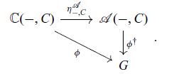
$\mathcal{A}$
-algebra. If
 $\phi \colon \mathbb{C}({-}, C) \to G$
is a morphism between presheaves, then there exists a unique homomorphism
$\phi \colon \mathbb{C}({-}, C) \to G$
is a morphism between presheaves, then there exists a unique homomorphism
 \begin{equation*} \phi^{\dagger} \colon \left\langle \mathcal{A} ({-}, C), \mu^{\mathcal{A}}_{{-}, C} \colon \mathcal{A} \circ \mathcal{A} ({-}, C) \Rightarrow \mathcal{A} ({-}, C) \right\rangle \to \left\langle G , \alpha \colon \mathcal{A} \circ G \Rightarrow G \right\rangle \end{equation*}
between
 $\mathcal{A}$
-algebras that makes the following diagram commute up to isomorphism:
$\mathcal{A}$
-algebras that makes the following diagram commute up to isomorphism:
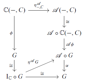
Proof We define
 $\phi^{\dagger} = \alpha \circ (\mathcal{A}\phi) \circ \rho^{-1} \colon \mathcal{A}({-}, C) \to G$
where
$\phi^{\dagger} = \alpha \circ (\mathcal{A}\phi) \circ \rho^{-1} \colon \mathcal{A}({-}, C) \to G$
where
 $\rho$
is the right unitor:
$\rho$
is the right unitor:

We check that
 $\phi^{\dagger}$
makes the diagram (3.3) commute. In the following diagram, the bottom triangle commutes by (3.1).
$\phi^{\dagger}$
makes the diagram (3.3) commute. In the following diagram, the bottom triangle commutes by (3.1).
To show that the above square commutes, it suffices to show the commutativity of the following diagram for each object A of
 $\mathbb{C}$
:
$\mathbb{C}$
:
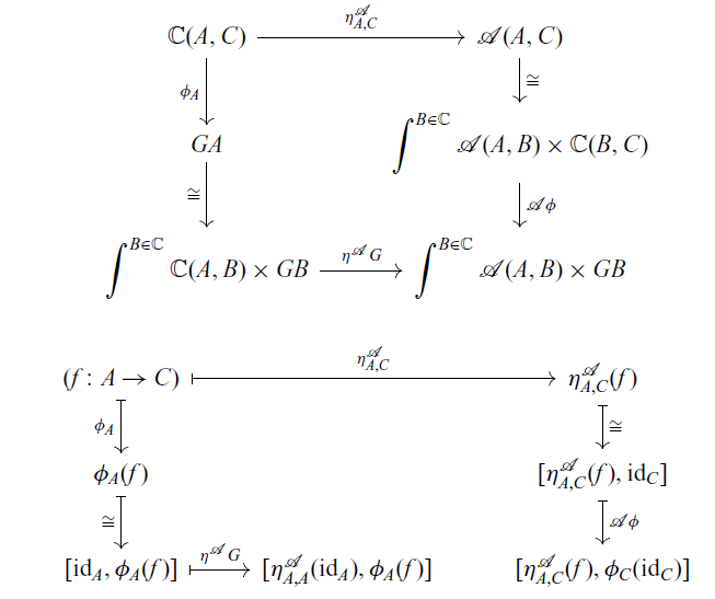
where [x, y] denotes the equivalence class of a pair (x, y), see the proof of Proposition A.3 in Appendix A. By chasing the diagram, it is enough to show
 $[\eta^{\mathcal{A}}_{A,A}(\mathrm{id}_A), \phi_A(f)] = [\eta^{\mathcal{A}}_{A,C}(f), \phi_C(\mathrm{id}_C)]$
in
$[\eta^{\mathcal{A}}_{A,A}(\mathrm{id}_A), \phi_A(f)] = [\eta^{\mathcal{A}}_{A,C}(f), \phi_C(\mathrm{id}_C)]$
in
 $\displaystyle \int^{B \in \mathbb{C}} \mathcal{A}(A, B) \times GB$
for each
$\displaystyle \int^{B \in \mathbb{C}} \mathcal{A}(A, B) \times GB$
for each
 $A \in \mathbb{C}$
and
$A \in \mathbb{C}$
and
 $f \colon A \to C$
. Consider the following commutative diagram.
$f \colon A \to C$
. Consider the following commutative diagram.
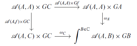
For
 $\langle \eta(\mathrm{id}_A) , \phi_C(\mathrm{id}_C) \rangle \in \mathcal{A}(A,A) \times GC$
, we have
$\langle \eta(\mathrm{id}_A) , \phi_C(\mathrm{id}_C) \rangle \in \mathcal{A}(A,A) \times GC$
, we have
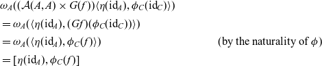 \begin{align*} & \omega_A( (\mathcal{A}(A,A) \times G(f)) \langle \eta(\mathrm{id}_A) , \phi_C(\mathrm{id}_C) \rangle) \\ & = \omega_A(\langle \eta(\mathrm{id}_A) , (Gf)(\phi_C(\mathrm{id}_C)) \rangle) \\ & = \omega_A(\langle \eta(\mathrm{id}_A) , \phi_C(f) \rangle) & \text{(by the naturality of $\phi$)}\\ & = [\eta(\mathrm{id}_A) , \phi_C(f) ] \end{align*}
and
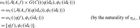 \begin{align*} & \omega_C( (\mathcal{A}(A,f) \times G(C)) \langle \eta(\mathrm{id}_A) , \phi_C(\mathrm{id}_C) \rangle) \\ & = \omega_C( \langle \mathcal{A}(A,f)(\eta(\mathrm{id}_A)) , \phi_C(\mathrm{id}_C) \rangle) \\ & = \omega_C( \langle \eta(f) , \phi_C(\mathrm{id}_C) \rangle) & \text{(by the naturality of $\eta_{A,{-}}$)} \\ & = [\eta(f) , \phi_C(\mathrm{id}_C)]. \end{align*}
Hence, we have
 $[\eta(\mathrm{id}_A), \phi(f)] = [\eta(f), \phi(\mathrm{id}_C)]$
.
$[\eta(\mathrm{id}_A), \phi(f)] = [\eta(f), \phi(\mathrm{id}_C)]$
.
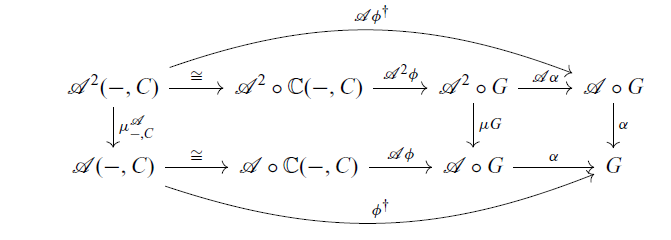
Next, we show that
 $\phi^{\dagger}$
is a homomorphism
$\phi^{\dagger}$
is a homomorphism
 $\mu^{\mathcal{A}}_{{-}, C} \to \alpha$
of
$\mu^{\mathcal{A}}_{{-}, C} \to \alpha$
of
 $\mathcal{A}$
-algebras. It suffices to show the commutativity of the left and right square in the following diagram. The right square commutes because
$\mathcal{A}$
-algebras. It suffices to show the commutativity of the left and right square in the following diagram. The right square commutes because
 $\alpha$
is an
$\alpha$
is an
 $\mathcal{A}$
-algebra (3.2), and the left square commutes by the naturality of
$\mathcal{A}$
-algebra (3.2), and the left square commutes by the naturality of
 $\mu$
and
$\mu$
and
 $\phi$
and some calculation similar to the above argument.
$\phi$
and some calculation similar to the above argument.
By the Yoneda lemma, giving a morphism
 $\phi \colon \mathbb{C}({-}, C) \to G$
between presheaves is equivalent to giving an element
$\phi \colon \mathbb{C}({-}, C) \to G$
between presheaves is equivalent to giving an element
 $p \in GC$
. In the proof of Theorem 3.3,
$p \in GC$
. In the proof of Theorem 3.3,
 $\phi^{\dagger}$
is defined by (3.4). Hence, for
$\phi^{\dagger}$
is defined by (3.4). Hence, for
 $a \in \mathcal{A}(A, C)$
,
$a \in \mathcal{A}(A, C)$
,
 $\phi^{\dagger}(a)$
is calculated to be
$\phi^{\dagger}(a)$
is calculated to be
 $\alpha([a, p])$
. In summary, we obtain the following corollary.
$\alpha([a, p])$
. In summary, we obtain the following corollary.
Corollary 3.4. Let
 $\mathcal{A}$
be a promonad on
$\mathcal{A}$
be a promonad on
 $\mathbb{C}$
,
$\mathbb{C}$
,
 $C \in \mathbb{C}$
, G be a presheaf on
$C \in \mathbb{C}$
, G be a presheaf on
 $\mathbb{C}$
, and
$\mathbb{C}$
, and
 $\langle G, \alpha \rangle$
be an
$\langle G, \alpha \rangle$
be an
 $\mathcal{A}$
-algebra. For an element
$\mathcal{A}$
-algebra. For an element
 $p \in GC$
, there is a homomorphism
$p \in GC$
, there is a homomorphism
 \begin{equation*} h \colon \left\langle \mathcal{A} ({-}, C), \mu^{\mathcal{A}}_{{-}, C} \colon \mathcal{A} \circ \mathcal{A} ({-}, C) \Rightarrow \mathcal{A}({-}, C) \right\rangle \to \left\langle G, \alpha \colon \mathcal{A} \circ G \Rightarrow G \right\rangle \end{equation*}
satisfying
 $h_{A}(a) = \alpha([a, p])$
for any
$h_{A}(a) = \alpha([a, p])$
for any
 $A \in \mathbb{C}$
and
$A \in \mathbb{C}$
and
 $a \in \mathcal{A}(A , C)$
, and
$a \in \mathcal{A}(A , C)$
, and
 $h(\eta^{\mathcal{A}}_{A,C}(f)) = (Gf)(p)$
for any
$h(\eta^{\mathcal{A}}_{A,C}(f)) = (Gf)(p)$
for any
 $A \in \mathbb{C}$
and
$A \in \mathbb{C}$
and
 $f \colon A \to C$
in
$f \colon A \to C$
in
 $\mathbb{C}$
.
$\mathbb{C}$
.
When G in Corollary 3.4 is a presheaf
 $\mathcal{A}'({-}, D)$
for another promonad
$\mathcal{A}'({-}, D)$
for another promonad ![]() and an object
and an object
 $D \in \mathbb{C}$
, we obtain the following corollary.
$D \in \mathbb{C}$
, we obtain the following corollary.
Corollary 3.5. Let
 $\mathcal{A}$
and
$\mathcal{A}$
and
 $\mathcal{A}'$
be promonads on
$\mathcal{A}'$
be promonads on
 $\mathbb{C}$
,
$\mathbb{C}$
,
 $D \in \mathbb{C}$
, and
$D \in \mathbb{C}$
, and
 $\alpha$
be a family
$\alpha$
be a family
 $(\alpha_{A, B} \colon \mathcal{A}(A, B) \times \mathcal{A}'(B, D) \to \mathcal{A}'(A, D))_{A, B \in \mathbb{C}}$
of maps which is natural in A and extranatural in B and satisfies (3.1) and (3.2) for
$(\alpha_{A, B} \colon \mathcal{A}(A, B) \times \mathcal{A}'(B, D) \to \mathcal{A}'(A, D))_{A, B \in \mathbb{C}}$
of maps which is natural in A and extranatural in B and satisfies (3.1) and (3.2) for
 $G = \mathcal{A}'({-}, D)$
. For an element
$G = \mathcal{A}'({-}, D)$
. For an element
 $p \in \mathcal{A}'(C,D)$
, there is a homomorphism
$p \in \mathcal{A}'(C,D)$
, there is a homomorphism
 \begin{equation*} h \colon \left\langle \mathcal{A}({-}, C), \mu^{\mathcal{A}} \right\rangle \to \left\langle \mathcal{A}'({-}, D), \alpha \right\rangle \end{equation*}
such that
 $h(a) = \alpha_{A,C}(a, p)$
for any
$h(a) = \alpha_{A,C}(a, p)$
for any
 $A \in \mathbb{C}$
and
$A \in \mathbb{C}$
and
 $a \in \mathcal{A}(A,C)$
, and
$a \in \mathcal{A}(A,C)$
, and
 $h_A(\eta^{\mathcal{A}}_{A,C}(f)) = \mathcal{A}'(f, D)(p)$
for any
$h_A(\eta^{\mathcal{A}}_{A,C}(f)) = \mathcal{A}'(f, D)(p)$
for any
 $A \in \mathbb{C}$
and
$A \in \mathbb{C}$
and
 $f \colon A \to C$
in
$f \colon A \to C$
in
 $\mathbb{C}$
.
$\mathbb{C}$
.
We use Corollary 3.5 to interpret handlers for arrows.
Remark 3.6. Note that we can prove Theorem 3.3 in another way. From the promonad ![]() , we can obtain a cocontinuous monad
, we can obtain a cocontinuous monad
 $\widetilde{\mathcal{A}} \colon [\mathbb{C}^{\mathrm{op}},\mathbf{Set}] \to [\mathbb{C}^{\mathrm{op}}, \mathbf{Set}]$
by the following construction. Then, using the universality of free
$\widetilde{\mathcal{A}} \colon [\mathbb{C}^{\mathrm{op}},\mathbf{Set}] \to [\mathbb{C}^{\mathrm{op}}, \mathbf{Set}]$
by the following construction. Then, using the universality of free
 $\widetilde{\mathcal{A}}$
-algebra, Theorem 3.3 is proved.
$\widetilde{\mathcal{A}}$
-algebra, Theorem 3.3 is proved.
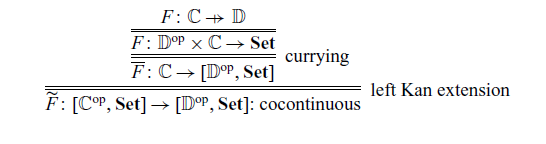
4 The arrow calculus with operations and handlers
The arrow calculus was introduced by Lindley et al. (Reference Lindley, Wadler and Yallop2010, Reference Lindley, Wadler and Yallop2011). We add operations and handlers to their calculus.
4.1 Syntax and typing rules
Let
 $\mathord{BType}$
be a set of base types, and
$\mathord{BType}$
be a set of base types, and
 $\Sigma$
be a set of operations. We assume that two base types
$\Sigma$
be a set of operations. We assume that two base types
 $\gamma$
(coarity) and
$\gamma$
(coarity) and
 $\delta$
(arity) are assigned for each operation
$\delta$
(arity) are assigned for each operation
 $\mathsf{op} \in \Sigma$
. We write
$\mathsf{op} \in \Sigma$
. We write ![]() when the coarity and arity of
when the coarity and arity of
 $\mathsf{op}$
are
$\mathsf{op}$
are
 $\gamma$
and
$\gamma$
and
 $\delta$
, respectively. The syntax is shown in Figure 2. The difference from the original arrow calculus (Lindley et al., Reference Lindley, Wadler and Yallop2010, Reference Lindley, Wadler and Yallop2011) is the addition of
$\delta$
, respectively. The syntax is shown in Figure 2. The difference from the original arrow calculus (Lindley et al., Reference Lindley, Wadler and Yallop2010, Reference Lindley, Wadler and Yallop2011) is the addition of
 $\mathsf{op}(M)$
,
$\mathsf{op}(M)$
,
 $\mathop{\mathbf{handle}} R \mathop{\mathbf{with}} H$
to the commands and handlers H.
$\mathop{\mathbf{handle}} R \mathop{\mathbf{with}} H$
to the commands and handlers H.
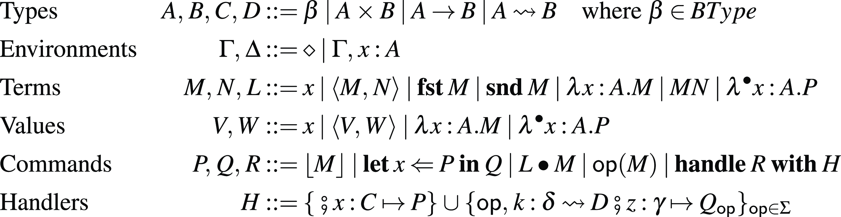
Fig. 2. The syntax of the arrow calculus with operations and handlers.
We call a type A primitive (written
 $\Phi(A)$
) if A is constructed only by
$\Phi(A)$
) if A is constructed only by
 $\beta$
,
$\beta$
,
 $\times$
and
$\times$
and
 $\to$
. Formally,
$\to$
. Formally,
 $\Phi(A)$
is defined as follows.
$\Phi(A)$
is defined as follows.
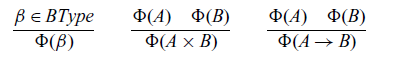
The typing rules for the arrow calculus are shown in Figure 3. The notion of primitive types is used in the rule ![]() .
.
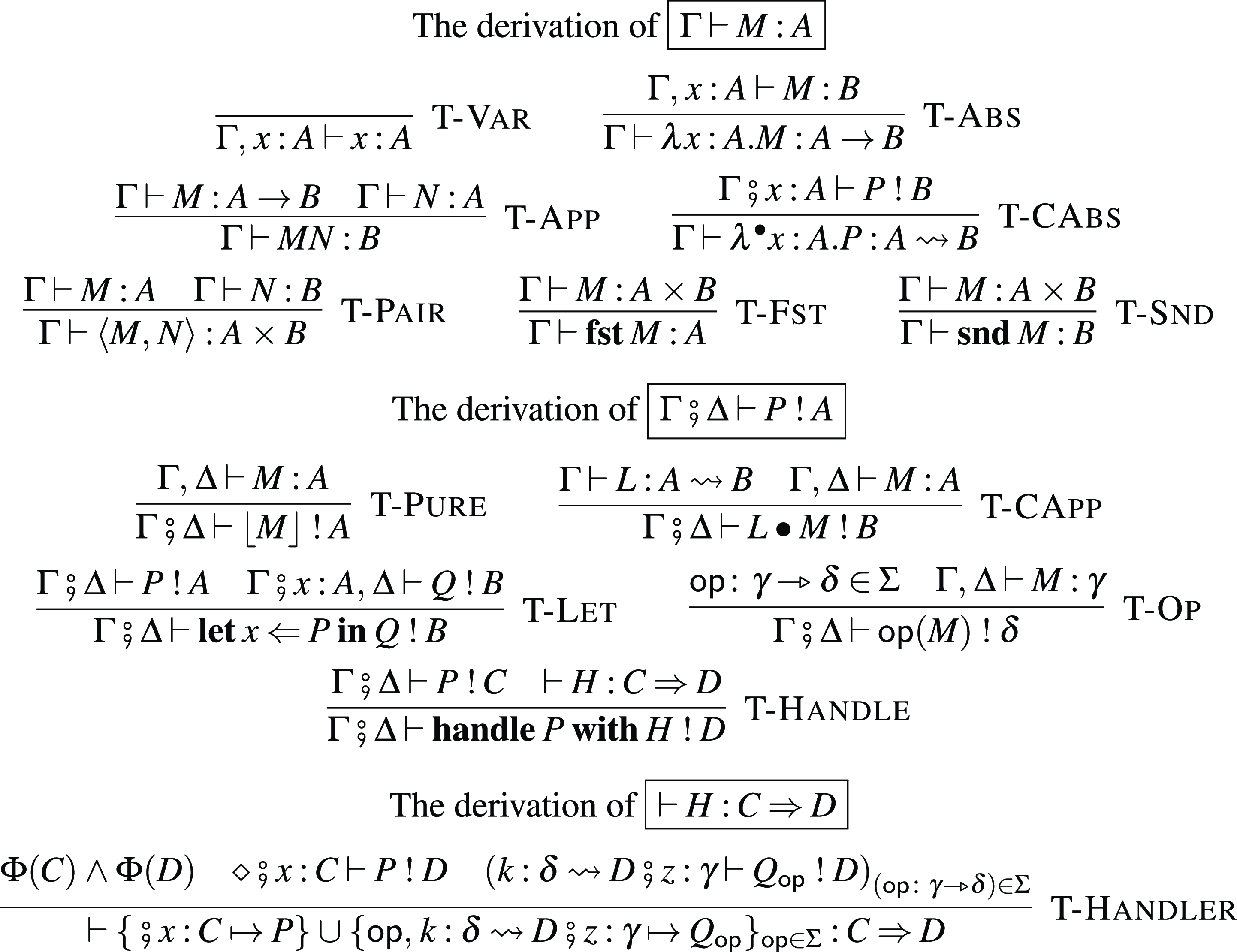
Fig. 3. Typing rules for the arrow calculus with operations and handlers.
A type
 $A \rightsquigarrow B$
is that of an effectful computation such that the type of its inputs is A and the type of its outputs is B.
$A \rightsquigarrow B$
is that of an effectful computation such that the type of its inputs is A and the type of its outputs is B.
As we described in Section 1.2.3, a term M is a pure function and a command P is an effectful computation. The command
 $\lfloor{M}\rfloor$
is a pure computation, which corresponds to
$\lfloor{M}\rfloor$
is a pure computation, which corresponds to
 $\mathtt{arr}$
in Haskell. The command
$\mathtt{arr}$
in Haskell. The command
 $L \bullet M$
is a command that invokes an arrow L with an input M. It corresponds to
$L \bullet M$
is a command that invokes an arrow L with an input M. It corresponds to
 $(\mathrel{>\!\!>\!\!>})$
and
$(\mathrel{>\!\!>\!\!>})$
and
 $\mathtt{arr}$
in Haskell. The command
$\mathtt{arr}$
in Haskell. The command
 $\mathop{\mathbf{let}} x \Leftarrow P \mathop{\mathbf{in}} Q$
is a sequential composition of commands P and Q, which corresponds to
$\mathop{\mathbf{let}} x \Leftarrow P \mathop{\mathbf{in}} Q$
is a sequential composition of commands P and Q, which corresponds to
 $(\mathrel{>\!\!>\!\!>})$
and
$(\mathrel{>\!\!>\!\!>})$
and
 $\mathtt{first}$
in Haskell. The command
$\mathtt{first}$
in Haskell. The command
 $\mathsf{op}(M)$
is an operation invocation with an input M.
$\mathsf{op}(M)$
is an operation invocation with an input M.
A judgement
 $\Gamma \vdash M : A$
for a term means that the term M is a pure function from
$\Gamma \vdash M : A$
for a term means that the term M is a pure function from
 $\Gamma$
to A. A judgement
$\Gamma$
to A. A judgement ![]() for a command means that the command P is a computation such that the type of its inputs is
for a command means that the command P is a computation such that the type of its inputs is
 $\Delta$
and the type of its outputs is A under the context
$\Delta$
and the type of its outputs is A under the context
 $\Gamma$
.
$\Gamma$
.
In the construction of handlers:
the command P corresponds to the
 $p \in \mathcal{A}'(C,D)$
in Corollary 3.5, and the family
$p \in \mathcal{A}'(C,D)$
in Corollary 3.5, and the family
 $\{ Q_{\mathsf{op}} \}_{\mathsf{op} \in \Sigma}$
of commands determines an algebraic structure
$\{ Q_{\mathsf{op}} \}_{\mathsf{op} \in \Sigma}$
of commands determines an algebraic structure
 $\alpha$
in Corollary 3.5.
$\alpha$
in Corollary 3.5.
Handlers for arrows are very similar to handlers for ordinary monads. The difference is that, in the handler (4.1),
 $x : C$
and
$x : C$
and
 $z : \gamma$
are not ordinary contexts, but inputs of the effectful computation P and
$z : \gamma$
are not ordinary contexts, but inputs of the effectful computation P and
 $Q_{\mathsf{op}}$
, respectively.
$Q_{\mathsf{op}}$
, respectively.
4.2 Operational semantics
We present the reduction rules for closed terms
 $\diamond \vdash M : A$
and closed commands
$\diamond \vdash M : A$
and closed commands ![]() . We define two kinds of evaluation contexts as follows.
. We define two kinds of evaluation contexts as follows.
 \begin{align*} \mathcal{E} & ::= [{-}] \mid \mathcal{E} N \mid V \mathcal{E} \mid \mathcal{E} \bullet N \mid (\lambda^{\bullet} x . P) \bullet \mathcal{E} \mid \lfloor{\mathcal{E}}\rfloor \mid \mathsf{op}(\mathcal{E}) \mid \mathop{\mathbf{fst}} \mathcal{E} \mid \mathop{\mathbf{snd}} \mathcal{E} \mid \langle {\mathcal{E}}, {M} \rangle \mid \langle {V}, {\mathcal{E}} \rangle \\ \mathcal{F} & ::= [{-}] \mid \mathop{\mathbf{let}} x \Leftarrow \mathcal{F} \mathop{\mathbf{in}} Q\end{align*}
We put a term in the hole of a context
 $\mathcal{E}[{-}]$
and a command in the hole of a context
$\mathcal{E}[{-}]$
and a command in the hole of a context
 $\mathcal{F}[{-}]$
. The reduction relation is shown in Figure 4.
$\mathcal{F}[{-}]$
. The reduction relation is shown in Figure 4.
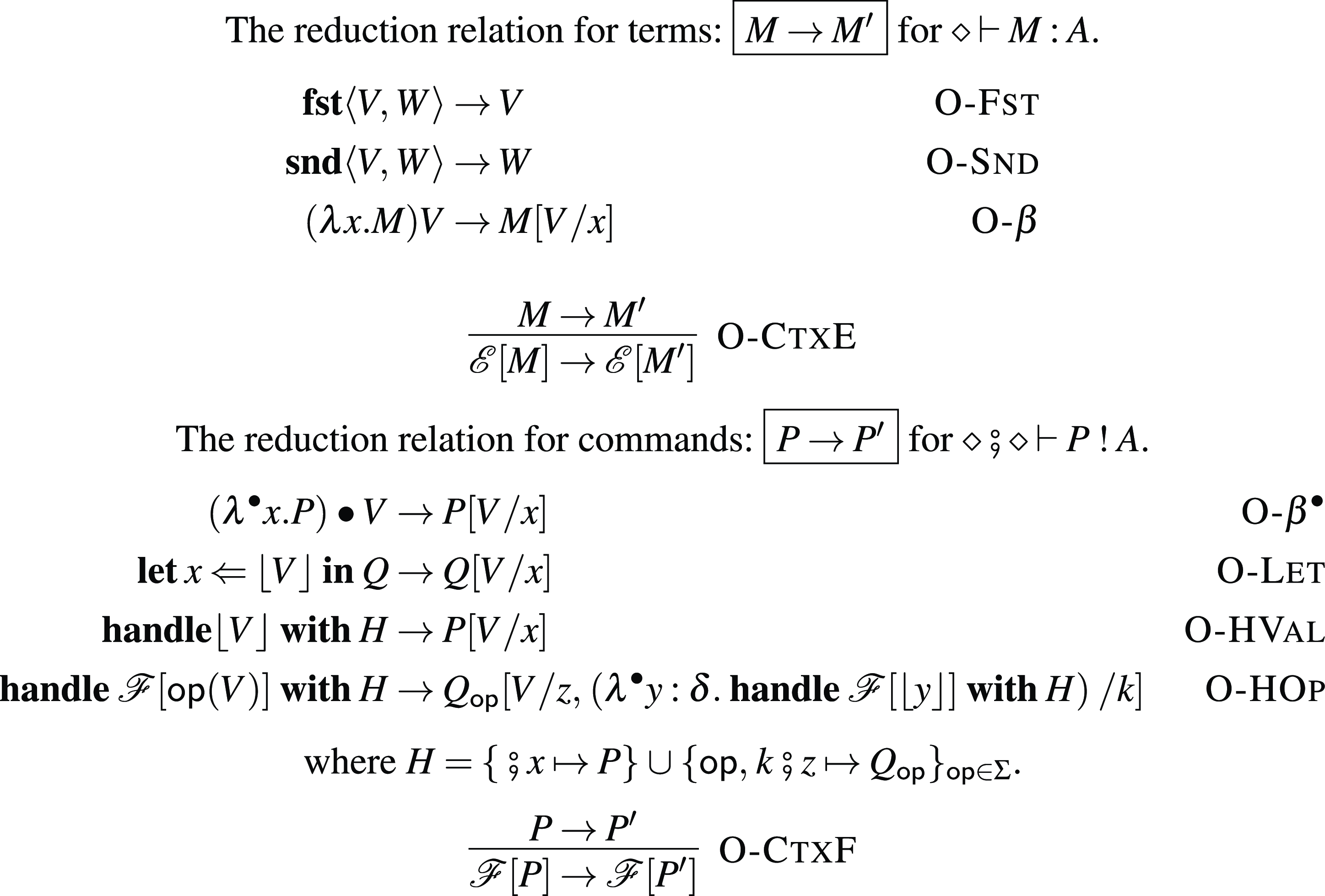
Fig. 4. Operational semantics.
Type preservation (Proposition 4.3) and progress (Proposition 4.1) hold for the arrow calculus with operations and handlers.
Proposition 4.1 (progress). The following hold.
-
1. For any well-typed term
$\diamond \vdash M : A$
, there exists a term M’ such that
$M \to M'$
or M is a value. -
2. For any well-typed command
, one of following holds.-
a. There exists a command P’ such that
$P \to P'$
. -
b.
$P = \lfloor{V}\rfloor$
for some value V. -
c.
$P = \mathcal{F}{[\mathsf{op}(V)]}$
for some operation
$\mathsf{op}$
, value V and context
$\mathcal{F}$
.
-


Lemma 4.2 (substitution) Let
 $\Gamma$
and
$\Gamma$
and
 $\Delta$
be contexts. The following hold.
$\Delta$
be contexts. The following hold.
-
1. If
$\Gamma, x : A \vdash M : B$
and
$\Gamma \vdash N : A$
are derivable, then
$\Gamma \vdash M[N / x] : B$
is derivable. -
2. If
and
$\Gamma \vdash N : A$
are derivable, then is derivable. -
3. If
and
$\Gamma, \Delta \vdash N : A$
are derivable, then is derivable.


Proof The proof is by induction on the derivations.
Proposition 4.3 (Type preservation) The following hold.
-
1. For any well-typed term
$\diamond \vdash M : A$
, if
$M \to M'$
then
$\diamond \vdash M' : A$
. -
2. For any well-typed command
, if
$P \to P'$
then .


Proof The proof is by induction on the derivation of
 $M \to M'$
and
$M \to M'$
and
 $P \to P'$
, and Lemma 4.2.
$P \to P'$
, and Lemma 4.2.
4.3 Example
In the description of handlers, clauses that just forward their input shall be omitted. For example, let
 $\Sigma = \{ \mathsf{op}_1, \mathsf{op}_2 \}$
, we write
$\Sigma = \{ \mathsf{op}_1, \mathsf{op}_2 \}$
, we write
for ![]() .
.
4.3.1 Logic circuit simulation
We explain the details of the example of logic circuit simulation in Section 1.2.3. Let
 $\mathord{BType} = \{ \mathrm{Bool} \}$
. The base type Bool is a type for boolean values. We add the following constants to the arrow calculus.
$\mathord{BType} = \{ \mathrm{Bool} \}$
. The base type Bool is a type for boolean values. We add the following constants to the arrow calculus.
 \begin{gather*} \mathtt{true} : \mathrm{Bool}, \quad \mathtt{false} : \mathrm{Bool}.\end{gather*}
Let
 ${\Sigma_{\mathrm{LC}}}$
be the signature of logic circuits defined in Section 1.2. We extend the arrow calculus by adding
${\Sigma_{\mathrm{LC}}}$
be the signature of logic circuits defined in Section 1.2. We extend the arrow calculus by adding
 $\mathop{\mathbf{if}} M \mathop{\mathbf{then}} N_1 \mathop{\mathbf{else}} N_2$
to terms with the following typing rule:
$\mathop{\mathbf{if}} M \mathop{\mathbf{then}} N_1 \mathop{\mathbf{else}} N_2$
to terms with the following typing rule:
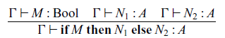
The operational semantics is extended by adding the following evaluation context and reduction relations.
 \begin{equation*} \mathcal{E} ::= \cdots \mid \mathop{\mathbf{if}} \mathcal{E} \mathop{\mathbf{then}} N_1 \mathop{\mathbf{else}} N_2,\end{equation*}
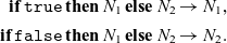 \begin{align*} \mathop{\mathbf{if}} \mathtt{true} \mathop{\mathbf{then}} N_1 \mathop{\mathbf{else}} N_2 & \to N_1, \\ \mathop{\mathbf{if}} \mathtt{false} \mathop{\mathbf{then}} N_1 \mathop{\mathbf{else}} N_2 & \to N_2.\end{align*}
Let
 $Q_{\mathsf{NAND}}$
be
$Q_{\mathsf{NAND}}$
be
 $\mathop{\mathbf{let}} u \Leftarrow \mathsf{AND}(z) \mathop{\mathbf{in}} \mathop{\mathbf{let}} v \Leftarrow \mathsf{NOT}(u) \mathop{\mathbf{in}} k \bullet v$
and
$\mathop{\mathbf{let}} u \Leftarrow \mathsf{AND}(z) \mathop{\mathbf{in}} \mathop{\mathbf{let}} v \Leftarrow \mathsf{NOT}(u) \mathop{\mathbf{in}} k \bullet v$
and
 $Q_{\mathsf{OR}}$
be
$Q_{\mathsf{OR}}$
be
 $\mathop{\mathbf{let}} u \Leftarrow \mathsf{NOT}(\mathop{\mathbf{fst}} z) \mathop{\mathbf{in}} \mathop{\mathbf{let}} v \Leftarrow \mathsf{NOT}(\mathop{\mathbf{snd}} z) \mathop{\mathbf{in}} \mathop{\mathbf{let}} w \Leftarrow \mathsf{AND}(\langle {u}, {v} \rangle) \mathop{\mathbf{in}} k \bullet w$
. The handler
$\mathop{\mathbf{let}} u \Leftarrow \mathsf{NOT}(\mathop{\mathbf{fst}} z) \mathop{\mathbf{in}} \mathop{\mathbf{let}} v \Leftarrow \mathsf{NOT}(\mathop{\mathbf{snd}} z) \mathop{\mathbf{in}} \mathop{\mathbf{let}} w \Leftarrow \mathsf{AND}(\langle {u}, {v} \rangle) \mathop{\mathbf{in}} k \bullet w$
. The handler ![]() and
and
 $H'_2$
defined in Section 1.2.3 is well-typed:
$H'_2$
defined in Section 1.2.3 is well-typed:
 $\vdash H'_1 : \mathrm{Bool} \Rightarrow \mathrm{Bool}$
and
$\vdash H'_1 : \mathrm{Bool} \Rightarrow \mathrm{Bool}$
and
 $\vdash H'_2 : \mathrm{Bool} \Rightarrow \mathrm{Bool}$
.
$\vdash H'_2 : \mathrm{Bool} \Rightarrow \mathrm{Bool}$
.
We check the derivation of
 $\vdash H'_1 : \mathrm{Bool} \Rightarrow \mathrm{Bool}$
. Let
$\vdash H'_1 : \mathrm{Bool} \Rightarrow \mathrm{Bool}$
. Let
 $\Gamma = k : \mathrm{Bool} \rightsquigarrow \mathrm{Bool}$
,
$\Gamma = k : \mathrm{Bool} \rightsquigarrow \mathrm{Bool}$
,
 $\Delta = z : \mathrm{Bool} \times \mathrm{Bool}$
and
$\Delta = z : \mathrm{Bool} \times \mathrm{Bool}$
and
 $\Delta' = (\Delta, u : \mathrm{Bool})$
. The derivation of
$\Delta' = (\Delta, u : \mathrm{Bool})$
. The derivation of ![]() is as follows.
is as follows.
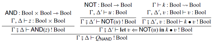
Similarly, we can derive ![]() . Hence, the derivation of
. Hence, the derivation of
 $\vdash H'_1 : \mathrm{Bool} \Rightarrow \mathrm{Bool}$
is as follows:
$\vdash H'_1 : \mathrm{Bool} \Rightarrow \mathrm{Bool}$
is as follows:
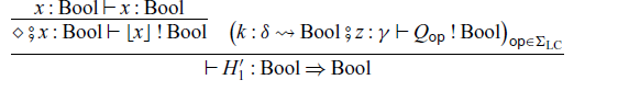
where
 $Q_{\mathsf{AND}} = \mathop{\mathbf{let}} u \Leftarrow \mathsf{AND}(z) \mathop{\mathbf{in}} k \bullet u$
and
$Q_{\mathsf{AND}} = \mathop{\mathbf{let}} u \Leftarrow \mathsf{AND}(z) \mathop{\mathbf{in}} k \bullet u$
and
 $Q_{\mathsf{NOT}} = \mathop{\mathbf{let}} u \Leftarrow \mathsf{NOT}(z) \mathop{\mathbf{in}} k \bullet u$
.
$Q_{\mathsf{NOT}} = \mathop{\mathbf{let}} u \Leftarrow \mathsf{NOT}(z) \mathop{\mathbf{in}} k \bullet u$
.
The evaluation of
 $\mathop{\mathbf{handle}} (\mathop{\mathbf{handle}} \mathsf{NAND}(\langle {\mathtt{true}}, {\mathtt{false}} \rangle) \mathop{\mathbf{with}} H'_1) \mathop{\mathbf{with}} H'_2$
is shown in Figure 5.
$\mathop{\mathbf{handle}} (\mathop{\mathbf{handle}} \mathsf{NAND}(\langle {\mathtt{true}}, {\mathtt{false}} \rangle) \mathop{\mathbf{with}} H'_1) \mathop{\mathbf{with}} H'_2$
is shown in Figure 5.
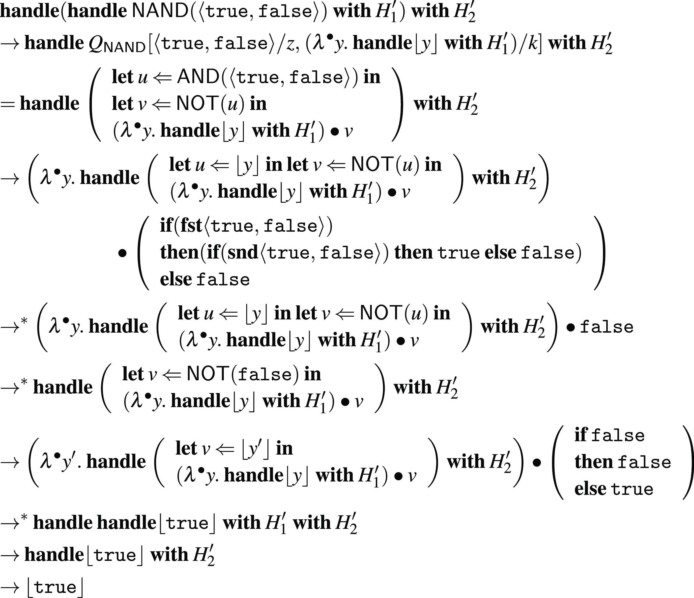
Fig. 5. The evaluation of
 $\mathop{\mathbf{handle}} (\mathop{\mathbf{handle}} \mathsf{NAND}(\langle {\mathtt{true}}, {\mathtt{false}} \rangle) \mathop{\mathbf{with}} H'_1) \mathop{\mathbf{with}} H'_2$
.
$\mathop{\mathbf{handle}} (\mathop{\mathbf{handle}} \mathsf{NAND}(\langle {\mathtt{true}}, {\mathtt{false}} \rangle) \mathop{\mathbf{with}} H'_1) \mathop{\mathbf{with}} H'_2$
.
4.3.2 Read only state
Let
 $\mathord{BType} = \{ \mathrm{Unit}, \mathrm{Bool} \}$
and
$\mathord{BType} = \{ \mathrm{Unit}, \mathrm{Bool} \}$
and ![]() . The operation
. The operation
 $\mathsf{get}$
is expected to read a state of type Bool and return the stored value. We can implement
$\mathsf{get}$
is expected to read a state of type Bool and return the stored value. We can implement
 $\mathsf{get}$
using a handler.
$\mathsf{get}$
using a handler.
The following judgements are derivable:
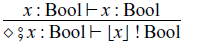

Hence, we can construct a handler ![]() and derive
and derive
 $\vdash H : \mathrm{Bool} \Rightarrow \mathrm{Bool}$
. This handler H implements
$\vdash H : \mathrm{Bool} \Rightarrow \mathrm{Bool}$
. This handler H implements
 $\mathsf{get}$
so that the stored value is
$\mathsf{get}$
so that the stored value is
 $\mathtt{true}$
. For example, the reduction of a program
$\mathtt{true}$
. For example, the reduction of a program
 $\mathop{\mathbf{handle}} \mathsf{get}(\mathtt{\langle\rangle}) \mathop{\mathbf{with}} H$
is as follows.
$\mathop{\mathbf{handle}} \mathsf{get}(\mathtt{\langle\rangle}) \mathop{\mathbf{with}} H$
is as follows.
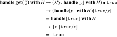 \begin{align*} \mathop{\mathbf{handle}} \mathsf{get}(\mathtt{\langle\rangle}) \mathop{\mathbf{with}} H & \to (\lambda^{\bullet} y . \mathop{\mathbf{handle}} \lfloor{y}\rfloor \mathop{\mathbf{with}} H) \bullet \mathtt{true} \\ & \to (\mathop{\mathbf{handle}} \lfloor{y}\rfloor \mathop{\mathbf{with}} H)[\mathtt{true} / y] \\ & = \mathop{\mathbf{handle}} \lfloor{\mathtt{true}}\rfloor \mathop{\mathbf{with}} H \\ & \to \lfloor{x}\rfloor[\mathtt{true} / x] \\ & = \lfloor{\mathtt{true}}\rfloor\end{align*}
5 Denotational semantics
5.1 Models of arrow calculus
We define models of the arrow calculus, in which the arrow calculus with operations is interpreted.
Definition 5.1 (a model of arrow calculus). A model of the arrow calculus consists of the following data.
-
• A cartesian closed category (ccc)
$\mathbb{C}$
. -
• A cocomplete cartesian closed category
$\mathbb{C}'$
. -
• A cartesian fully faithful functor
$J \colon \mathbb{C} \to \mathbb{C}'$
. -
• A
$\mathbb{C}$
-small strong promonad on
$\mathbb{C}$
in
$\mathbb{C}'$
-
$\mathbf{Prof}$
(Definitions 2.3 and 2.7).


For a ccc
 $\mathbb{C}$
, a cocomplete ccc
$\mathbb{C}$
, a cocomplete ccc
 $\mathbb{C}'$
and a cartesian fully faithful functor
$\mathbb{C}'$
and a cartesian fully faithful functor
 $J \colon \mathbb{C} \to \mathbb{C}'$
, the identity
$J \colon \mathbb{C} \to \mathbb{C}'$
, the identity
 $\mathbb{C}'$
-profunctor
$\mathbb{C}'$
-profunctor ![]() on
on
 $\mathbb{C}$
defined by
$\mathbb{C}$
defined by
 $\mathrm{I}_{\mathbb{C}}(A, B) = (JA \Rightarrow JB) = J(A \Rightarrow B)$
is a
$\mathrm{I}_{\mathbb{C}}(A, B) = (JA \Rightarrow JB) = J(A \Rightarrow B)$
is a
 $\mathbb{C}$
-small strong promonad on
$\mathbb{C}$
-small strong promonad on
 $\mathbb{C}$
in
$\mathbb{C}$
in
 $\mathbb{C}'$
-
$\mathbb{C}'$
-
 $\mathbf{Prof}$
. We have
$\mathbf{Prof}$
. We have
 $\mathrm{I}_{\mathbb{C}}^{\circ}(A, B) = (A \Rightarrow B)$
and
$\mathrm{I}_{\mathbb{C}}^{\circ}(A, B) = (A \Rightarrow B)$
and
 $J \circ \mathrm{I}_{\mathbb{C}}^{\circ} = \mathrm{I}_{\mathbb{C}}$
:
$J \circ \mathrm{I}_{\mathbb{C}}^{\circ} = \mathrm{I}_{\mathbb{C}}$
:
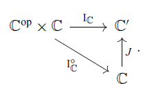
Definition 5.2 (interpretation.) Given a model of arrow calculus
 $(\mathbb{C}, \mathbb{C}', J, \mathcal{A})$
, interpretation
$(\mathbb{C}, \mathbb{C}', J, \mathcal{A})$
, interpretation
 $\mathord{\left[\![{\beta}\right]\!]} \in \mathbb{C}$
of each base type
$\mathord{\left[\![{\beta}\right]\!]} \in \mathbb{C}$
of each base type
 $\beta \in \mathord{BType}$
and interpretation
$\beta \in \mathord{BType}$
and interpretation
 $\mathord{\left[\![{\mathrm{op}}\right]\!]} \colon \mathcal{A}(\mathord{\left[\![{\delta}\right]\!]}, {-}) \Rightarrow \mathcal{A}(\mathord{\left[\![{\gamma}\right]\!]}, {-})$
of each operation
$\mathord{\left[\![{\mathrm{op}}\right]\!]} \colon \mathcal{A}(\mathord{\left[\![{\delta}\right]\!]}, {-}) \Rightarrow \mathcal{A}(\mathord{\left[\![{\gamma}\right]\!]}, {-})$
of each operation ![]() , we define interpretation of the arrow calculus with operations (without handlers). The interpretation
, we define interpretation of the arrow calculus with operations (without handlers). The interpretation
 $\mathord{\left[\![{A}\right]\!]}$
of a type A is defined as a natural extension of
$\mathord{\left[\![{A}\right]\!]}$
of a type A is defined as a natural extension of
 $\mathord{\left[\![{\beta}\right]\!]}$
with
$\mathord{\left[\![{\beta}\right]\!]}$
with
 $\mathord{\left[\![{A \rightsquigarrow B}\right]\!]} = \mathcal{A}^{\circ}(\mathord{\left[\![{A}\right]\!]}, \mathord{\left[\![{B}\right]\!]})$
. For a term
$\mathord{\left[\![{A \rightsquigarrow B}\right]\!]} = \mathcal{A}^{\circ}(\mathord{\left[\![{A}\right]\!]}, \mathord{\left[\![{B}\right]\!]})$
. For a term
 $\Gamma \vdash M : A$
and a command
$\Gamma \vdash M : A$
and a command ![]() , their interpretation
, their interpretation
 $\mathord{\left[\![{M}\right]\!]} \colon \mathord{\left[\![{\Gamma}\right]\!]} \to \mathord{\left[\![{A}\right]\!]}$
in
$\mathord{\left[\![{M}\right]\!]} \colon \mathord{\left[\![{\Gamma}\right]\!]} \to \mathord{\left[\![{A}\right]\!]}$
in
 $\mathbb{C}$
and
$\mathbb{C}$
and
 $\mathord{\left[\![{P}\right]\!]} \colon \mathord{\left[\![{\Gamma}\right]\!]} \to \mathcal{A}^{\circ}(\mathord{\left[\![{\Delta}\right]\!]}, \mathord{\left[\![{A}\right]\!]})$
in
$\mathord{\left[\![{P}\right]\!]} \colon \mathord{\left[\![{\Gamma}\right]\!]} \to \mathcal{A}^{\circ}(\mathord{\left[\![{\Delta}\right]\!]}, \mathord{\left[\![{A}\right]\!]})$
in
 $\mathbb{C}$
are defined as in Figure 6.
$\mathbb{C}$
are defined as in Figure 6.
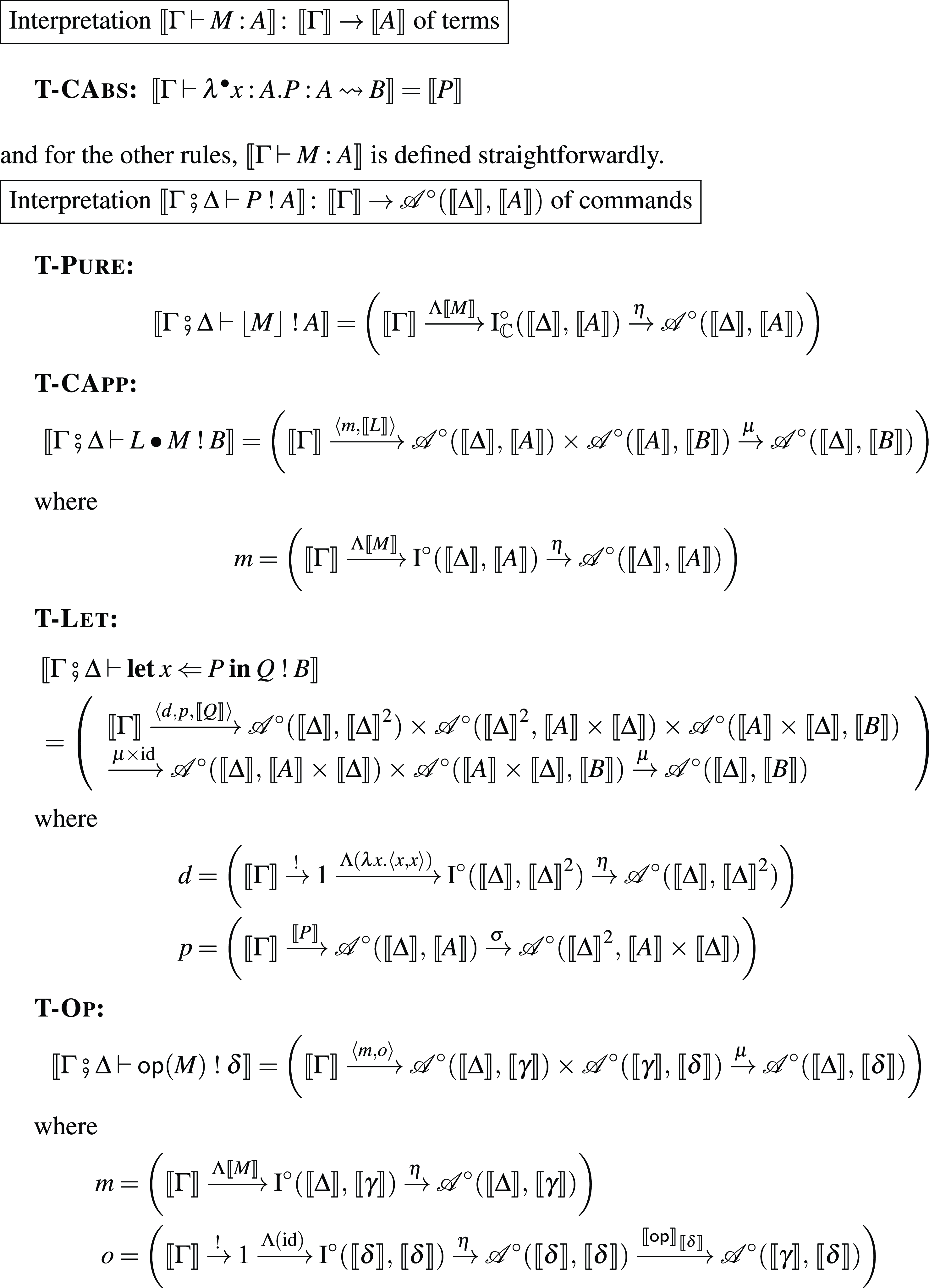
Fig. 6. The categorical semantics.
We discuss interpretation of handlers in Section 5.3.
5.2 Construction of a model of the arrow calculus
We give a semantics of the arrow calculus with operations and handlers using a
 $\mathbf{Set}$
-small strong
$\mathbf{Set}$
-small strong
 $\mathbf{Ens}$
-promonad
$\mathbf{Ens}$
-promonad
 $\mathcal{A}$
on
$\mathcal{A}$
on
 $\mathbf{Set}$
. We fix an interpretation of the base types
$\mathbf{Set}$
. We fix an interpretation of the base types
 $\mathord{\left[\![{{-}}\right]\!]} \colon \mathord{BType} \to \mathbf{Set}$
. Here
$\mathord{\left[\![{{-}}\right]\!]} \colon \mathord{BType} \to \mathbf{Set}$
. Here
 $\mathord{BType}$
is regarded as a discrete category.
$\mathord{BType}$
is regarded as a discrete category.
First, we construct a map
 $\mathrm{Arr}_{\Sigma} \colon \mathrm{Ob}(\mathbf{Set}^{\mathrm{op}}) \times \mathrm{Ob}(\mathbf{Set}) \to \mathrm{Ob}(\mathbf{Ens})$
.
$\mathrm{Arr}_{\Sigma} \colon \mathrm{Ob}(\mathbf{Set}^{\mathrm{op}}) \times \mathrm{Ob}(\mathbf{Set}) \to \mathrm{Ob}(\mathbf{Ens})$
.
Definition 5.3 (arrow term). For sets A and B,
 $\mathrm{Arr}_{\Sigma}(A, B)$
is defined to be the smallest class satisfying the rules in Figure 7. We call an element in
$\mathrm{Arr}_{\Sigma}(A, B)$
is defined to be the smallest class satisfying the rules in Figure 7. We call an element in
 $\mathrm{Arr}_{\Sigma}(A, B)$
an arrow term. An equation is a pair of arrow terms (t, t’) where
$\mathrm{Arr}_{\Sigma}(A, B)$
an arrow term. An equation is a pair of arrow terms (t, t’) where
 $t, t' \in \mathrm{Arr}_{\Sigma}(A, B)$
for some sets A and B. A theory is a pair
$t, t' \in \mathrm{Arr}_{\Sigma}(A, B)$
for some sets A and B. A theory is a pair
 $(\Sigma, E)$
of a signature
$(\Sigma, E)$
of a signature
 $\Sigma$
and a set E of equations.
$\Sigma$
and a set E of equations.
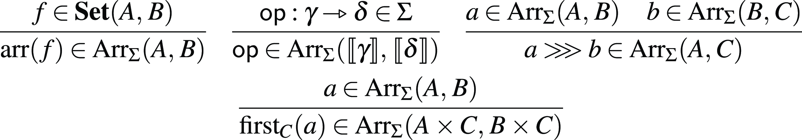
Fig. 7. Construction of
 $\mathrm{Arr}_{\Sigma}(A, B) \in \mathbf{Ens}$
for
$\mathrm{Arr}_{\Sigma}(A, B) \in \mathbf{Ens}$
for
 $A, B \in \mathbf{Set}$
.
$A, B \in \mathbf{Set}$
.
In the following, we consider only the case
 $E = \emptyset$
.
$E = \emptyset$
.
Unfortunately,
 $\mathrm{Arr}_{\Sigma}(A, B)$
is a proper class because it contains
$\mathrm{Arr}_{\Sigma}(A, B)$
is a proper class because it contains
 $a \mathrel{>\!\!>\!\!>} b$
for any
$a \mathrel{>\!\!>\!\!>} b$
for any
 $X \in \mathbf{Set}$
,
$X \in \mathbf{Set}$
,
 $a \in \mathrm{Arr}_{\Sigma}(A, X)$
and
$a \in \mathrm{Arr}_{\Sigma}(A, X)$
and
 $b \in \mathrm{Arr}_{\Sigma}(X, B)$
. However, we can define an equivalence relation
$b \in \mathrm{Arr}_{\Sigma}(X, B)$
. However, we can define an equivalence relation
 $\sim$
on
$\sim$
on
 $\mathrm{Arr}_{\Sigma}(A, B)$
and obtain
$\mathrm{Arr}_{\Sigma}(A, B)$
and obtain
 $\mathbf{Set}$
-small strong
$\mathbf{Set}$
-small strong
 $\mathbf{Ens}$
-promonad
$\mathbf{Ens}$
-promonad ![]() .
.
The equivalence relation
 $\sim$
is defined as the smallest congruence relation satisfying the following axioms (5.1)–(5.9), which correspond to the arrow laws (1.1)–(1.9).
$\sim$
is defined as the smallest congruence relation satisfying the following axioms (5.1)–(5.9), which correspond to the arrow laws (1.1)–(1.9).
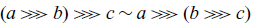 \begin{align} (a \mathrel{>\!\!>\!\!>} b) \mathrel{>\!\!>\!\!>} c & \sim a \mathrel{>\!\!>\!\!>} (b \mathrel{>\!\!>\!\!>} c)\end{align}
 \begin{align}\mathop{\mathrm{arr}}\nolimits(g \circ f) & \sim \mathop{\mathrm{arr}}\nolimits(f) \mathrel{>\!\!>\!\!>} \mathop{\mathrm{arr}}\nolimits(g)\end{align}
 \begin{align}\mathop{\mathrm{arr}}\nolimits(\mathrm{id}) \mathrel{>\!\!>\!\!>} a & \sim a\end{align}
 \begin{align}a \mathrel{>\!\!>\!\!>} \mathop{\mathrm{arr}}\nolimits(\mathrm{id}) & \sim a\end{align}
 \begin{align}\mathop{\mathrm{first}}\nolimits(a) \mathrel{>\!\!>\!\!>} \mathop{\mathrm{arr}}\nolimits(\mathrm{id} \times f) & \sim \mathop{\mathrm{arr}}\nolimits(\mathrm{id} \times f) \mathrel{>\!\!>\!\!>} \mathop{\mathrm{first}}\nolimits(a)\end{align}
 \begin{align}\mathop{\mathrm{first}}\nolimits(a) \mathrel{>\!\!>\!\!>} \mathop{\mathrm{arr}}\nolimits(\pi_1) & \sim \mathop{\mathrm{arr}}\nolimits(\pi_1) \mathrel{>\!\!>\!\!>} a\end{align}
 \begin{align}\mathop{\mathrm{first}}\nolimits(a) \mathrel{>\!\!>\!\!>} \mathop{\mathrm{arr}}\nolimits(\alpha) & \sim \mathop{\mathrm{arr}}\nolimits(\alpha) \mathrel{>\!\!>\!\!>} \mathop{\mathrm{first}}\nolimits(\mathop{\mathrm{first}}\nolimits(a))\end{align}
 \begin{align}\mathop{\mathrm{first}}\nolimits (\mathop{\mathrm{arr}}\nolimits(f)) & \sim \mathop{\mathrm{arr}}\nolimits(f \times \mathrm{id})\end{align}
 \begin{align}\mathop{\mathrm{first}}\nolimits (a \mathrel{>\!\!>\!\!>} b) & \sim \mathop{\mathrm{first}}\nolimits(a) \mathrel{>\!\!>\!\!>} \mathop{\mathrm{first}}\nolimits(b)\end{align}
We denote
 $\mathrm{Arr}_{\Sigma}(A, B) / {\sim}$
as
$\mathrm{Arr}_{\Sigma}(A, B) / {\sim}$
as
 $\mathcal{A}_{\Sigma}(A, B)$
. We define
$\mathcal{A}_{\Sigma}(A, B)$
. We define
 $\mathop{\mathrm{second}}\nolimits_X(a) = \mathop{\mathrm{arr}}\nolimits(\mathop{sym}_{X, A}) \mathrel{>\!\!>\!\!>} \mathop{\mathrm{first}}\nolimits_X(a) \mathrel{>\!\!>\!\!>} \mathop{\mathrm{arr}}\nolimits(\mathop{sym}_{X, B})$
for
$\mathop{\mathrm{second}}\nolimits_X(a) = \mathop{\mathrm{arr}}\nolimits(\mathop{sym}_{X, A}) \mathrel{>\!\!>\!\!>} \mathop{\mathrm{first}}\nolimits_X(a) \mathrel{>\!\!>\!\!>} \mathop{\mathrm{arr}}\nolimits(\mathop{sym}_{X, B})$
for
 $a \in \mathrm{Arr}_{\Sigma}(A, B)$
, where the map
$a \in \mathrm{Arr}_{\Sigma}(A, B)$
, where the map
 $\mathop{sym}_{Y, Z} \colon Y \times Z \to Z \times Y$
is defined by
$\mathop{sym}_{Y, Z} \colon Y \times Z \to Z \times Y$
is defined by
 $\mathop{sym}_{Y,Z}(y,z) = (z, y)$
.
$\mathop{sym}_{Y,Z}(y,z) = (z, y)$
.
We use string diagram like notation introduced by Asada and Hasuo (Reference Asada and Hasuo2010). Arrow terms are depicted as follows.
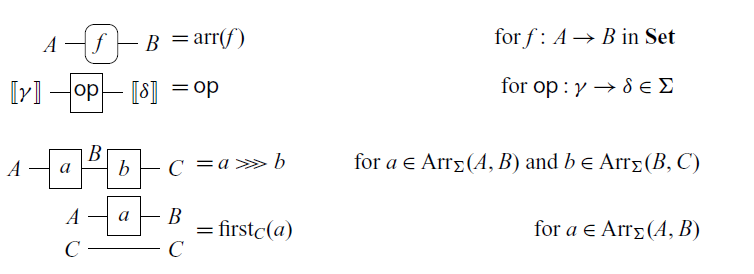
Especially, we write
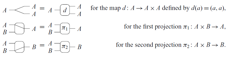
The
 $\mathbf{Set}$
-smallness of
$\mathbf{Set}$
-smallness of
 $\mathrm{Arr}({-}_1, {-}_2) / \sim$
is proven from Proposition 5.5. It says that every arrow term is equivalent to the normal form. The normal form was introduced by Yallop (Reference Yallop2010) for arrows in Haskell to compare two programs. The normal form here is essentially the same as his except that it is defined for arrow terms
$\mathrm{Arr}({-}_1, {-}_2) / \sim$
is proven from Proposition 5.5. It says that every arrow term is equivalent to the normal form. The normal form was introduced by Yallop (Reference Yallop2010) for arrows in Haskell to compare two programs. The normal form here is essentially the same as his except that it is defined for arrow terms
 $a \in \mathrm{Arr}_{\Sigma}(A, B)$
. The size of the collection of all normal forms is small.
$a \in \mathrm{Arr}_{\Sigma}(A, B)$
. The size of the collection of all normal forms is small.
Definition 5.4 (normal form.) Let n be a natural number, ![]() be a sequence of operations,
be a sequence of operations,
 $(f_i \colon \mathord{\left[\![{\delta_{i-1}}\right]\!]} \times \cdots \times \mathord{\left[\![{\delta_{1}}\right]\!]} \times A \to \mathord{\left[\![{\gamma_i}\right]\!]})_{i = 1}^n$
be a sequence of maps and
$(f_i \colon \mathord{\left[\![{\delta_{i-1}}\right]\!]} \times \cdots \times \mathord{\left[\![{\delta_{1}}\right]\!]} \times A \to \mathord{\left[\![{\gamma_i}\right]\!]})_{i = 1}^n$
be a sequence of maps and
 $g \colon \mathord{\left[\![{\delta_n}\right]\!]} \times \cdots \times \mathord{\left[\![{\delta_1}\right]\!]} \times A \to B$
. We define an arrow term
$g \colon \mathord{\left[\![{\delta_n}\right]\!]} \times \cdots \times \mathord{\left[\![{\delta_1}\right]\!]} \times A \to B$
. We define an arrow term
 $\mathop{\mathsf{nf}}\left({(\mathsf{op}_i)_{i = 1}^{n}}, {(f_i)_{i = 1}^n}; {g}\right)$
inductively as follows:
$\mathop{\mathsf{nf}}\left({(\mathsf{op}_i)_{i = 1}^{n}}, {(f_i)_{i = 1}^n}; {g}\right)$
inductively as follows:
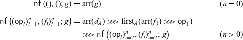 \begin{align*} \mathop{\mathsf{nf}}\left({()}, {()}; {g}\right) = & \mathop{\mathrm{arr}}\nolimits(g) & (n = 0) \\[0.5em] \mathop{\mathsf{nf}}\left({(\mathsf{op}_i)_{i = 1}^{n}}, {(f_i)_{i = 1}^{n}}; {g}\right) = & \mathop{\mathrm{arr}}\nolimits(d_A) \mathrel{>\!\!>\!\!>} \mathop{\mathrm{first}}\nolimits_A( \mathop{\mathrm{arr}}\nolimits(f_1) \mathrel{>\!\!>\!\!>} \mathsf{op}_1 ) \\ & \mathrel{>\!\!>\!\!>} \mathop{\mathsf{nf}}\left({(\mathsf{op}_i)_{i = 2}^n}, {(f_i)_{i = 2}^n}; {g}\right) & (n > 0) \end{align*}
where
 $d_X \colon X \to X \times X$
is the diagonal map:
$d_X \colon X \to X \times X$
is the diagonal map:
 $d_X(x) = (x, x)$
. We call
$d_X(x) = (x, x)$
. We call
 $\mathop{\mathsf{nf}}\left({(\mathsf{op}_i)_{i=1}^n}, {(f_i)_{i=1}^n}; {g}\right)$
a normal form.
$\mathop{\mathsf{nf}}\left({(\mathsf{op}_i)_{i=1}^n}, {(f_i)_{i=1}^n}; {g}\right)$
a normal form.
Proposition 5.5. Let A and B be sets. For any
 $a \in \mathrm{Arr}_{\Sigma}(A, B)$
, there exist a natural number
$a \in \mathrm{Arr}_{\Sigma}(A, B)$
, there exist a natural number
 $n \in \mathbb{N}$
, a sequence of operations
$n \in \mathbb{N}$
, a sequence of operations ![]() , a sequence of maps
, a sequence of maps
 $(f_i \colon \mathord{\left[\![{\delta_{i-1}}\right]\!]} \times \cdots \times \mathord{\left[\![{\delta_{1}}\right]\!]} \times A \to \mathord{\left[\![{\gamma_i}\right]\!]})_{i = 1 , \dots, n}$
and
$(f_i \colon \mathord{\left[\![{\delta_{i-1}}\right]\!]} \times \cdots \times \mathord{\left[\![{\delta_{1}}\right]\!]} \times A \to \mathord{\left[\![{\gamma_i}\right]\!]})_{i = 1 , \dots, n}$
and
 $g \colon \mathord{\left[\![{\delta_n}\right]\!]} \times \cdots \times \mathord{\left[\![{\delta_1}\right]\!]} \times A \to B$
such that
$g \colon \mathord{\left[\![{\delta_n}\right]\!]} \times \cdots \times \mathord{\left[\![{\delta_1}\right]\!]} \times A \to B$
such that
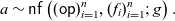 \begin{equation*} a \sim \mathop{\mathsf{nf}}\left({(\mathsf{op})_{i=1}^n}, {(f_i)_{i=1}^n}; {g}\right). \end{equation*}
Proof sketch We prove by induction on the structure of
 $a \in \mathrm{Arr}_{\Sigma}(A, B)$
. Since the proof is very long, we only prove the following two cases here and the rest of the proof is sent to the appendix.
$a \in \mathrm{Arr}_{\Sigma}(A, B)$
. Since the proof is very long, we only prove the following two cases here and the rest of the proof is sent to the appendix.
In case
 $a = \mathop{\mathrm{arr}}\nolimits(f)$
for some
$a = \mathop{\mathrm{arr}}\nolimits(f)$
for some
 $f \colon A \to B$
. The proposition trivially holds for
$f \colon A \to B$
. The proposition trivially holds for
 $n = 0$
.
$n = 0$
.
In case
 $a = \mathsf{op}$
for some
$a = \mathsf{op}$
for some ![]() with
with
 $\mathord{\left[\![{\gamma}\right]\!]} = A$
and
$\mathord{\left[\![{\gamma}\right]\!]} = A$
and
 $\mathord{\left[\![{\delta}\right]\!]} = B$
. We have
$\mathord{\left[\![{\delta}\right]\!]} = B$
. We have
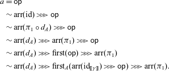 \begin{align*} a & = \mathsf{op} \\ & \sim \mathop{\mathrm{arr}}\nolimits(\mathrm{id}) \mathrel{>\!\!>\!\!>} \mathsf{op} \\ & \sim \mathop{\mathrm{arr}}\nolimits(\pi_1 \circ d_{A}) \mathrel{>\!\!>\!\!>} \mathsf{op} \\ & \sim \mathop{\mathrm{arr}}\nolimits(d_A) \mathrel{>\!\!>\!\!>} \mathop{\mathrm{arr}}\nolimits(\pi_1) \mathrel{>\!\!>\!\!>} \mathsf{op} \\ & \sim \mathop{\mathrm{arr}}\nolimits(d_A) \mathrel{>\!\!>\!\!>} \mathop{\mathrm{first}}\nolimits(\mathsf{op}) \mathrel{>\!\!>\!\!>} \mathop{\mathrm{arr}}\nolimits(\pi_1) \\ & \sim \mathop{\mathrm{arr}}\nolimits(d_{A}) \mathrel{>\!\!>\!\!>} \mathop{\mathrm{first}}\nolimits_A(\mathop{\mathrm{arr}}\nolimits(\mathrm{id}_{\mathord{\left[\![{\gamma}\right]\!]}}) \mathrel{>\!\!>\!\!>} \mathsf{op}) \mathrel{>\!\!>\!\!>} \mathop{\mathrm{arr}}\nolimits(\pi_1). \end{align*}
See Figure 8.
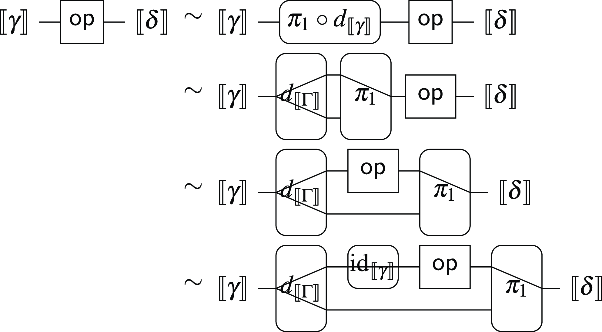
Fig. 8. In case
 $a = \mathsf{op}$
.
$a = \mathsf{op}$
.
The collection
 $\mathcal{A}^{\circ}_{\Sigma}(A, B)$
of all normal forms in
$\mathcal{A}^{\circ}_{\Sigma}(A, B)$
of all normal forms in
 $\mathrm{Arr}_{\Sigma}(A, B)$
is a set, not a proper class, because
$\mathrm{Arr}_{\Sigma}(A, B)$
is a set, not a proper class, because
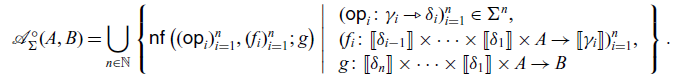
We identify an equivalence class [a] for an arrow term
 $a \in \mathrm{Arr}_{\Sigma}(A,B)$
with its normal form.
$a \in \mathrm{Arr}_{\Sigma}(A,B)$
with its normal form.
The map
 $\mathcal{A}_{\Sigma} \colon \mathrm{Ob}(\mathbf{Set}^{\mathrm{op}}) \times \mathrm{Ob}(\mathbf{Set}) \to \mathrm{Ob}(\mathbf{Ens})$
is extended to an
$\mathcal{A}_{\Sigma} \colon \mathrm{Ob}(\mathbf{Set}^{\mathrm{op}}) \times \mathrm{Ob}(\mathbf{Set}) \to \mathrm{Ob}(\mathbf{Ens})$
is extended to an
 $\mathbf{Ens}$
-profunctor
$\mathbf{Ens}$
-profunctor ![]() by defining
by defining
 $\mathcal{A}_{\Sigma}(f,g)([a]) = [\mathop{\mathrm{arr}}\nolimits(f) \mathrel{>\!\!>\!\!>} a \mathrel{>\!\!>\!\!>} \mathop{\mathrm{arr}}\nolimits(g)]$
for
$\mathcal{A}_{\Sigma}(f,g)([a]) = [\mathop{\mathrm{arr}}\nolimits(f) \mathrel{>\!\!>\!\!>} a \mathrel{>\!\!>\!\!>} \mathop{\mathrm{arr}}\nolimits(g)]$
for
 $f \colon A' \to A$
,
$f \colon A' \to A$
,
 $g \colon B \to B'$
and
$g \colon B \to B'$
and
 $a \in \mathrm{Arr}_{\Sigma}(A, B)$
. We have constructed a model of the arrow calculus.
$a \in \mathrm{Arr}_{\Sigma}(A, B)$
. We have constructed a model of the arrow calculus.
Proposition 5.6. The data
 $(\mathbf{Set}, \mathbf{Ens}, J, \mathcal{A}_{\Sigma})$
is a model of the arrow calculus (Definition 5.1).
$(\mathbf{Set}, \mathbf{Ens}, J, \mathcal{A}_{\Sigma})$
is a model of the arrow calculus (Definition 5.1).
Note that the model
 $(\mathbf{Set}, \mathbf{Ens}, J, \mathcal{A}_{\Sigma})$
is the free model in the sense that if
$(\mathbf{Set}, \mathbf{Ens}, J, \mathcal{A}_{\Sigma})$
is the free model in the sense that if
 $(\mathbf{Set}, \mathbf{Ens}, J, \mathcal{A})$
is also a model and a family
$(\mathbf{Set}, \mathbf{Ens}, J, \mathcal{A})$
is also a model and a family ![]() of interpretation of operations is specified, then there is a unique 2-cell
of interpretation of operations is specified, then there is a unique 2-cell
 $h \colon \mathcal{A}_{\Sigma} \Rightarrow \mathcal{A}$
which is compatible with units and multiplications of
$h \colon \mathcal{A}_{\Sigma} \Rightarrow \mathcal{A}$
which is compatible with units and multiplications of
 $\mathcal{A}_{\Sigma}$
and
$\mathcal{A}_{\Sigma}$
and
 $\mathcal{A}$
.
$\mathcal{A}$
.
5.3 Interpretation of handlers
We interpret handlers in the model
 $(\mathbf{Set}, \mathbf{Ens}, J, \mathcal{A}_{\Sigma})$
of the arrow calculus. We fix an interpretation of base types
$(\mathbf{Set}, \mathbf{Ens}, J, \mathcal{A}_{\Sigma})$
of the arrow calculus. We fix an interpretation of base types
 $\mathord{\left[\![{{-}}\right]\!]} \colon \mathord{BType} \to \mathrm{Ob}(\mathbf{Set})$
.
$\mathord{\left[\![{{-}}\right]\!]} \colon \mathord{BType} \to \mathrm{Ob}(\mathbf{Set})$
.
5.3.1 The problem of strength
Unlike in the case of the strong monad
 $\mathcal{T} \colon \mathbf{Set} \to \mathbf{Set}$
in
$\mathcal{T} \colon \mathbf{Set} \to \mathbf{Set}$
in
 $\mathbf{Cat}$
, in the case of the strong promonad
$\mathbf{Cat}$
, in the case of the strong promonad ![]() in
in
 $\mathbf{Ens}$
-
$\mathbf{Ens}$
-
 $\mathbf{Prof}$
, the treatment of the strength is non-trivial. To interpret a handler as a
$\mathbf{Prof}$
, the treatment of the strength is non-trivial. To interpret a handler as a
 $\mathcal{A}_{\Sigma}^{\circ}$
-homomorphism, we have to construct a family of maps
$\mathcal{A}_{\Sigma}^{\circ}$
-homomorphism, we have to construct a family of maps
 \begin{equation} \left( \alpha_{A, B} \colon \mathcal{A}_{\Sigma}^{\circ}(A , B) \times \mathcal{A}_{\Sigma}^{\circ}(B, \mathord{\left[\![{D}\right]\!]}) \to \mathcal{A}_{\Sigma}^{\circ}(A, \mathord{\left[\![{D}\right]\!]}) \right)_{A, B}\end{equation}
from a handler ![]() :
:
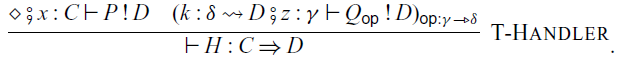
The problem is that we cannot define the maps (5.10) since there is no way to define
 $\alpha(\mathop{\mathrm{first}}\nolimits_S(\mathsf{op}), b)$
for
$\alpha(\mathop{\mathrm{first}}\nolimits_S(\mathsf{op}), b)$
for ![]() and
and
 $b \in \mathcal{A}_{\Sigma}^{\circ}(\mathord{\left[\![{\delta}\right]\!]} \times S, \mathord{\left[\![{D}\right]\!]})$
:
$b \in \mathcal{A}_{\Sigma}^{\circ}(\mathord{\left[\![{\delta}\right]\!]} \times S, \mathord{\left[\![{D}\right]\!]})$
:
 \begin{equation} \begin{split} \mathcal{A}_{\Sigma}^{\circ}(\mathord{\left[\![{\gamma}\right]\!]} \times S, \mathord{\left[\![{\delta}\right]\!]} \times S) \times \mathcal{A}_{\Sigma}^{\circ}(\mathord{\left[\![{\delta}\right]\!]} \times S, \mathord{\left[\![{D}\right]\!]}) & \to \mathcal{A}_{\Sigma}^{\circ}(\mathord{\left[\![{\gamma}\right]\!]} \times S, \mathord{\left[\![{D}\right]\!]}) \\ (\mathop{\mathrm{first}}\nolimits_S(\mathsf{op}), b) & \mapsto \alpha(\mathop{\mathrm{first}}\nolimits_S(\mathsf{op}), b). \end{split}\end{equation}
To define the above map, we need maps
 $\mathcal{A}_{\Sigma}^{\circ}(\mathord{\left[\![{\delta}\right]\!]} \times S, \mathord{\left[\![{D}\right]\!]}) \to \mathcal{A}_{\Sigma}^{\circ}(\mathord{\left[\![{\gamma}\right]\!]} \times S, \mathord{\left[\![{D}\right]\!]})$
as an interpretation of
$\mathcal{A}_{\Sigma}^{\circ}(\mathord{\left[\![{\delta}\right]\!]} \times S, \mathord{\left[\![{D}\right]\!]}) \to \mathcal{A}_{\Sigma}^{\circ}(\mathord{\left[\![{\gamma}\right]\!]} \times S, \mathord{\left[\![{D}\right]\!]})$
as an interpretation of
 $Q_{\mathsf{op}}$
. However, in the naïve interpretation (Definition 5.2), the command
$Q_{\mathsf{op}}$
. However, in the naïve interpretation (Definition 5.2), the command
 $Q_{\mathsf{op}}$
is interpreted as a map
$Q_{\mathsf{op}}$
is interpreted as a map
 $\mathord{\left[\![{Q_{\mathsf{op}}}\right]\!]} \colon \mathcal{A}_{\Sigma}^{\circ}(\mathord{\left[\![{\delta}\right]\!]}, \mathord{\left[\![{D}\right]\!]}) \to \mathcal{A}_{\Sigma}^{\circ}(\mathord{\left[\![{\gamma}\right]\!]}, \mathord{\left[\![{D}\right]\!]})$
.
$\mathord{\left[\![{Q_{\mathsf{op}}}\right]\!]} \colon \mathcal{A}_{\Sigma}^{\circ}(\mathord{\left[\![{\delta}\right]\!]}, \mathord{\left[\![{D}\right]\!]}) \to \mathcal{A}_{\Sigma}^{\circ}(\mathord{\left[\![{\gamma}\right]\!]}, \mathord{\left[\![{D}\right]\!]})$
.
5.3.2 Interpretation with a parameter
We solve this problem by using an additional parameter
 $S \in \mathrm{Ob}(\mathbf{Set})$
in the interpretation of terms. This additional parameter enables us to define maps
$S \in \mathrm{Ob}(\mathbf{Set})$
in the interpretation of terms. This additional parameter enables us to define maps
 $\mathcal{A}_{\Sigma}^{\circ}(\mathord{\left[\![{\delta}\right]\!]} \times S, \mathord{\left[\![{D}\right]\!]}) \to \mathcal{A}_{\Sigma}^{\circ}(\mathord{\left[\![{\gamma}\right]\!]} \times S, \mathord{\left[\![{D}\right]\!]})$
as an interpretation of
$\mathcal{A}_{\Sigma}^{\circ}(\mathord{\left[\![{\delta}\right]\!]} \times S, \mathord{\left[\![{D}\right]\!]}) \to \mathcal{A}_{\Sigma}^{\circ}(\mathord{\left[\![{\gamma}\right]\!]} \times S, \mathord{\left[\![{D}\right]\!]})$
as an interpretation of
 $Q_{\mathsf{op}}$
. For a type A and a set S, we define the interpretation
$Q_{\mathsf{op}}$
. For a type A and a set S, we define the interpretation
 $\mathord{\left[\![{A}\right]\!]}^S$
as an extension of
$\mathord{\left[\![{A}\right]\!]}^S$
as an extension of
 $\mathord{\left[\![{\beta}\right]\!]}$
for
$\mathord{\left[\![{\beta}\right]\!]}$
for
 $\beta \in \mathord{BType}$
.
$\beta \in \mathord{BType}$
.
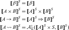 \begin{align*} \mathord{\left[\![{\beta}\right]\!]}^S & = \mathord{\left[\![{\beta}\right]\!]} \\ \mathord{\left[\![{A \times B}\right]\!]}^S & = \mathord{\left[\![{A}\right]\!]}^S \times \mathord{\left[\![{B}\right]\!]}^S \\ \mathord{\left[\![{A \to B}\right]\!]}^S & = \mathord{\left[\![{A}\right]\!]}^S \Rightarrow \mathord{\left[\![{B}\right]\!]}^S \\ \mathord{\left[\![{A \rightsquigarrow B}\right]\!]}^S & = \mathcal{A}_{\Sigma}^{\circ}(\mathord{\left[\![{A}\right]\!]}^S \times S, \mathord{\left[\![{B}\right]\!]}^S)\end{align*}
The interpretation
 $\mathord{\left[\![{\Gamma}\right]\!]}^S$
of a context
$\mathord{\left[\![{\Gamma}\right]\!]}^S$
of a context
 $\Gamma$
is defined as an extension of the interpretation of types:
$\Gamma$
is defined as an extension of the interpretation of types:
 \begin{equation*} \mathord{\left[\![{\diamond}\right]\!]}^S = 1, \qquad \mathord{\left[\![{\Gamma, x : A}\right]\!]}^S = \mathord{\left[\![{\Gamma}\right]\!]}^S \times \mathord{\left[\![{A}\right]\!]}^S.\end{equation*}
The key is the interpretation
 $\mathord{\left[\![{A \rightsquigarrow B}\right]\!]}^S$
of a type
$\mathord{\left[\![{A \rightsquigarrow B}\right]\!]}^S$
of a type
 $A \rightsquigarrow B$
. Adding S to the “input argument” of the arrow allows us to deal with strength.
$A \rightsquigarrow B$
. Adding S to the “input argument” of the arrow allows us to deal with strength.
If a type A is primitive, its interpretation is independent of S, that is we can show the following lemma by the definitions.
Lemma 5.7. If a type A is primitive (
 $\Phi(A)$
), then
$\Phi(A)$
), then
 $\mathord{\left[\![{A}\right]\!]}^S = \mathord{\left[\![{A}\right]\!]}^1$
for any S.
$\mathord{\left[\![{A}\right]\!]}^S = \mathord{\left[\![{A}\right]\!]}^1$
for any S.
Next, we define interpretation of terms and commands. For judgements
 $\Gamma \vdash M : A$
and
$\Gamma \vdash M : A$
and ![]() , we want to define:
, we want to define:
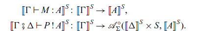
Let
 $e \in \mathord{\left[\![{\Gamma}\right]\!]}^S$
. The interpretation of terms is defined as follows. In the following, definitions are described by elements of sets, rather than by morphisms as in Figure 6. This is to avoid making the definition of interpretation of handlers more complex than necessary.
$e \in \mathord{\left[\![{\Gamma}\right]\!]}^S$
. The interpretation of terms is defined as follows. In the following, definitions are described by elements of sets, rather than by morphisms as in Figure 6. This is to avoid making the definition of interpretation of handlers more complex than necessary.
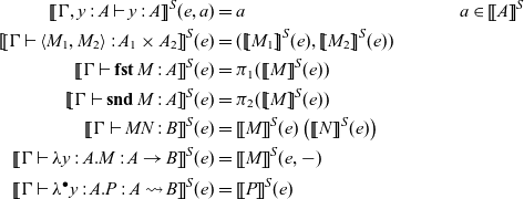 \begin{align*} \mathord{\left[\![{\Gamma, y : A \vdash y : A}\right]\!]}^S(e, a) & = a & a \in \mathord{\left[\![{A}\right]\!]}^S \\ \mathord{\left[\![{\Gamma \vdash \langle {M_1}, {M_2} \rangle : A_1 \times A_2}\right]\!]}^S(e) & = (\mathord{\left[\![{M_1}\right]\!]}^S(e) , \mathord{\left[\![{M_2}\right]\!]}^S(e)) \\ \mathord{\left[\![{\Gamma \vdash \mathop{\mathbf{fst}}{M} : A}\right]\!]}^S(e) & = \pi_1 (\mathord{\left[\![{M}\right]\!]}^S(e)) \\ \mathord{\left[\![{\Gamma \vdash \mathop{\mathbf{snd}}{M} : A}\right]\!]}^S(e) & = \pi_2 (\mathord{\left[\![{M}\right]\!]}^S(e)) \\ \mathord{\left[\![{\Gamma \vdash MN : B}\right]\!]}^S(e) & = \mathord{\left[\![{M}\right]\!]}^S(e)\left(\mathord{\left[\![{N}\right]\!]}^S(e)\right) \\ \mathord{\left[\![{\Gamma \vdash \lambda y : A . M : A \to B}\right]\!]}^S(e) & = \mathord{\left[\![{M}\right]\!]}^S(e, {-}) \\ \mathord{\left[\![{\Gamma \vdash \lambda^{\bullet} y : A . P : A \rightsquigarrow B}\right]\!]}^S(e) & = \mathord{\left[\![{P}\right]\!]}^S(e)\end{align*}
The interpretation of commands is defined as follows.
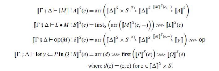
The interpretation of
 $\mathord{\left[\![{\mathop{\mathbf{let}} y \Leftarrow P \mathop{\mathbf{in}} Q}\right]\!]}^S(e)$
is illustrated as follows.
$\mathord{\left[\![{\mathop{\mathbf{let}} y \Leftarrow P \mathop{\mathbf{in}} Q}\right]\!]}^S(e)$
is illustrated as follows.
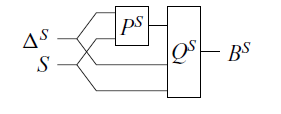
To interpret handling ![]() , we construct an algebra from
, we construct an algebra from ![]() . Note that the derivation is
. Note that the derivation is
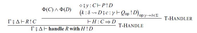
By Lemma 5.7, we have
 $\mathord{\left[\![{C}\right]\!]}^S = \mathord{\left[\![{C}\right]\!]}^1$
and
$\mathord{\left[\![{C}\right]\!]}^S = \mathord{\left[\![{C}\right]\!]}^1$
and
 $\mathord{\left[\![{D}\right]\!]}^S = \mathord{\left[\![{D}\right]\!]}^1$
. We have maps:
$\mathord{\left[\![{D}\right]\!]}^S = \mathord{\left[\![{D}\right]\!]}^1$
. We have maps:
The maps
 $\mathord{\left[\![{Q_{\mathsf{op}}}\right]\!]}^S$
induce an
$\mathord{\left[\![{Q_{\mathsf{op}}}\right]\!]}^S$
induce an
 $\mathcal{A}_{\Sigma}$
-algebra
$\mathcal{A}_{\Sigma}$
-algebra
 $\alpha$
on the presheaf
$\alpha$
on the presheaf
 $\mathcal{A}_{\Sigma}({-}, \mathord{\left[\![{D}\right]\!]})$
as follows.
$\mathcal{A}_{\Sigma}({-}, \mathord{\left[\![{D}\right]\!]})$
as follows.
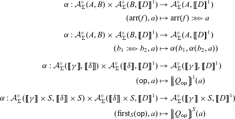 \begin{align*} \alpha : \mathcal{A}_{\Sigma}^{\circ}(A, B) \times \mathcal{A}_{\Sigma}^{\circ}(B, \mathord{\left[\![{D}\right]\!]}^1) & \to \mathcal{A}_{\Sigma}^{\circ}(A, \mathord{\left[\![{D}\right]\!]}^1) \\ (\mathop{\mathrm{arr}}\nolimits(f) , a) & \mapsto \mathop{\mathrm{arr}}\nolimits(f) \mathrel{>\!\!>\!\!>} a \\[0.5em] \alpha : \mathcal{A}_{\Sigma}^{\circ}(A, B) \times \mathcal{A}_{\Sigma}^{\circ}(B, \mathord{\left[\![{D}\right]\!]}^1) & \to \mathcal{A}_{\Sigma}^{\circ}(A, \mathord{\left[\![{D}\right]\!]}^1) \\ (b_1 \mathrel{>\!\!>\!\!>} b_2 , a) & \mapsto \alpha(b_1 , \alpha(b_2, a)) \\[0.5em] \alpha : \mathcal{A}_{\Sigma}^{\circ}(\mathord{\left[\![{\gamma}\right]\!]}, \mathord{\left[\![{\delta}\right]\!]}) \times \mathcal{A}_{\Sigma}^{\circ}(\mathord{\left[\![{\delta}\right]\!]}, \mathord{\left[\![{D}\right]\!]}^1) & \to \mathcal{A}_{\Sigma}^{\circ}(\mathord{\left[\![{\gamma}\right]\!]}, \mathord{\left[\![{D}\right]\!]}^1) \\ (\mathsf{op} , a) & \mapsto \mathord{\left[\![{Q_{\mathsf{op}}}\right]\!]}^1(a) \\[0.5em] \alpha : \mathcal{A}_{\Sigma}^{\circ}(\mathord{\left[\![{\gamma}\right]\!]} \times S, \mathord{\left[\![{\delta}\right]\!]} \times S) \times \mathcal{A}_{\Sigma}^{\circ}(\mathord{\left[\![{\delta}\right]\!]} \times S, \mathord{\left[\![{D}\right]\!]}^1) & \to \mathcal{A}_{\Sigma}^{\circ}(\mathord{\left[\![{\gamma}\right]\!]} \times S, \mathord{\left[\![{D}\right]\!]}^1) \\ (\mathop{\mathrm{first}}\nolimits_S(\mathsf{op}) , a) & \mapsto \mathord{\left[\![{Q_{\mathsf{op}}}\right]\!]}^S(a) \\[0.5em]\end{align*}
Note that, since every arrow term is equivalent to a normal form (Proposition 5.5),
 $\alpha(b, a)$
is well defined.
$\alpha(b, a)$
is well defined.
We also have
 $\mathord{\left[\![{P}\right]\!]}^1 \in \mathcal{A}_{\Sigma}(\mathord{\left[\![{C}\right]\!]}^1 , \mathord{\left[\![{D}\right]\!]}^1)$
. Hence, by Corollary 3.5, there exists a homomorphism
$\mathord{\left[\![{P}\right]\!]}^1 \in \mathcal{A}_{\Sigma}(\mathord{\left[\![{C}\right]\!]}^1 , \mathord{\left[\![{D}\right]\!]}^1)$
. Hence, by Corollary 3.5, there exists a homomorphism
 $h \colon \mu \to \alpha$
such that the following diagram commutes:
$h \colon \mu \to \alpha$
such that the following diagram commutes:
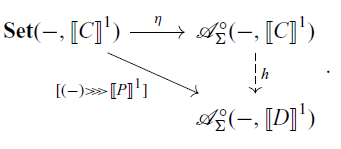
We use the homomorphism h to interpret
 $\mathop{\mathbf{handle}} R \mathop{\mathbf{with}} H$
:
$\mathop{\mathbf{handle}} R \mathop{\mathbf{with}} H$
:
and write
 $\mathord{\left[\![{H}\right]\!]}$
for the homomorphism h.
$\mathord{\left[\![{H}\right]\!]}$
for the homomorphism h.
The denotational semantics
 $\mathord{\left[\![{{-}}\right]\!]}^S$
defined here is compatible with the categorical semantics
$\mathord{\left[\![{{-}}\right]\!]}^S$
defined here is compatible with the categorical semantics
 $\mathord{\left[\![{{-}}\right]\!]}$
(Definition 5.2) in the model
$\mathord{\left[\![{{-}}\right]\!]}$
(Definition 5.2) in the model
 $(\mathbf{Set}, \mathbf{Ens}, J, \mathcal{A}_{\Sigma})$
in the following sense.
$(\mathbf{Set}, \mathbf{Ens}, J, \mathcal{A}_{\Sigma})$
in the following sense.
Proposition 5.8. Let
 $\Gamma$
and
$\Gamma$
and
 $\Delta$
be primitive contexts and A be a primitive type. Let M be a term and P be a command of the arrow calculus with operations (without handlers). The following hold.
$\Delta$
be primitive contexts and A be a primitive type. Let M be a term and P be a command of the arrow calculus with operations (without handlers). The following hold.
-
1. If
$\Gamma \vdash M : A$
then
$\mathord{\left[\![{M}\right]\!]}^S = \mathord{\left[\![{M}\right]\!]}$
for any S. -
2. If
then
$(\mathop{\mathrm{arr}}\nolimits(j_s) \mathrel{>\!\!>\!\!>} \mathord{\left[\![{P}\right]\!]}^S(e)) = \mathord{\left[\![{P}\right]\!]}(e)$
for any S,
$s \in S$
and
$e \in \mathord{\left[\![{\Gamma}\right]\!]}$
where
$j_s(z) = (z , s)$
for
$z \in \mathord{\left[\![{\Delta}\right]\!]}$
.


Proposition 5.9. Let
 $\Gamma$
and
$\Gamma$
and
 $\Delta$
be contexts and A be a type. Let M be a term and P be a command of the arrow calculus with operations (without handlers). The following hold.
$\Delta$
be contexts and A be a type. Let M be a term and P be a command of the arrow calculus with operations (without handlers). The following hold.
-
1. If
$\Gamma \vdash M : A$
then
$\mathord{\left[\![{M}\right]\!]}^1 = \mathord{\left[\![{M}\right]\!]}$
. -
2. If
then
$\mathord{\left[\![{P}\right]\!]}^1 = \mathord{\left[\![{P}\right]\!]}$
.


Hence, we write
 $\mathord{\left[\![{A}\right]\!]}^1$
and
$\mathord{\left[\![{A}\right]\!]}^1$
and
 $\mathord{\left[\![{\Gamma}\right]\!]}^1$
simply as
$\mathord{\left[\![{\Gamma}\right]\!]}^1$
simply as
 $\mathord{\left[\![{A}\right]\!]}$
and
$\mathord{\left[\![{A}\right]\!]}$
and
 $\mathord{\left[\![{\Gamma}\right]\!]}$
, respectively.
$\mathord{\left[\![{\Gamma}\right]\!]}$
, respectively.
Remark 5.10. Let
 $\mathbb{C}$
be a cartesian closed category,
$\mathbb{C}$
be a cartesian closed category,
 $\mathbb{C}'$
be a cocomplete cartesian closed category and
$\mathbb{C}'$
be a cocomplete cartesian closed category and
 $J \colon \mathbb{C} \to \mathbb{C}'$
be a strong cartesian fully faithful functor. For an ordinary strong monad
$J \colon \mathbb{C} \to \mathbb{C}'$
be a strong cartesian fully faithful functor. For an ordinary strong monad
 $\mathcal{T} \colon \mathbb{C} \to \mathbb{C}$
, we do not have the problem on the strength. The reason is as follows. Let
$\mathcal{T} \colon \mathbb{C} \to \mathbb{C}$
, we do not have the problem on the strength. The reason is as follows. Let ![]() be a strong promonad
be a strong promonad
 ${\mathcal{T}}_{*}$
(Proposition 2.4) in
${\mathcal{T}}_{*}$
(Proposition 2.4) in ![]() defined by
defined by
 \begin{equation*} \mathcal{A}(A, B) = \mathbb{C}(A, \mathcal{T} B) = (JA \Rightarrow J\mathcal{T} B) \in \mathbb{C}' \end{equation*}
for a strong monad
 $\mathcal{T} \colon \mathbb{C} \to \mathbb{C}$
. This promonad
$\mathcal{T} \colon \mathbb{C} \to \mathbb{C}$
. This promonad
 $\mathcal{A}$
is
$\mathcal{A}$
is
 $\mathbb{C}$
-small. Judgements
$\mathbb{C}$
-small. Judgements ![]() are interpreted as morphisms
are interpreted as morphisms
 \begin{equation*} \mathord{\left[\![{Q_{\mathsf{op}}}\right]\!]} \colon \mathord{\left[\![{\gamma}\right]\!]} \times (\mathord{\left[\![{\delta}\right]\!]} \Rightarrow \mathcal{T} \mathord{\left[\![{D}\right]\!]}) \to \mathcal{T} \mathord{\left[\![{D}\right]\!]}, \qquad \mathsf{op} \in \Sigma \end{equation*}
in
 $\mathbb{C}$
. An
$\mathbb{C}$
. An
 $\mathcal{A}$
-algebra
$\mathcal{A}$
-algebra
 $\alpha$
can be constructed from the set of morphisms
$\alpha$
can be constructed from the set of morphisms
 $\{ \mathord{\left[\![{Q_{\mathsf{op}}}\right]\!]} \}_{\mathsf{op} \in \Sigma}$
. The map (5.11) is defined as follows.
$\{ \mathord{\left[\![{Q_{\mathsf{op}}}\right]\!]} \}_{\mathsf{op} \in \Sigma}$
. The map (5.11) is defined as follows.
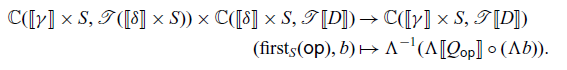 \begin{equation} \begin{split} \mathbb{C}(\mathord{\left[\![{\gamma}\right]\!]} \times S, \mathcal{T}(\mathord{\left[\![{\delta}\right]\!]} \times S)) \times \mathbb{C}(\mathord{\left[\![{\delta}\right]\!]} \times S, \mathcal{T} \mathord{\left[\![{D}\right]\!]}) & \to \mathbb{C}(\mathord{\left[\![{\gamma}\right]\!]} \times S, \mathcal{T} \mathord{\left[\![{D}\right]\!]}) \\ (\mathop{\mathrm{first}}\nolimits_S(\mathsf{op}), b) & \mapsto \Lambda^{-1}( \Lambda \mathord{\left[\![{Q_{\mathsf{op}}}\right]\!]} \circ (\Lambda b)). \end{split} \end{equation}
The key is that if
 $\mathcal{A}(A, B) = \mathbb{C}(A, \mathcal{T} B)$
, we have
$\mathcal{A}(A, B) = \mathbb{C}(A, \mathcal{T} B)$
, we have
 \begin{equation} \mathcal{L}_{A, B, C} \colon \mathcal{A}^{\circ}(C \times A, B) \cong \mathcal{A}^{\circ}(C, \mathcal{A}^{\circ}(A, B)) \qquad \text{for any $A, B, C \in \mathbb{C}$.} \end{equation}
Conversely, assume that (5.13) holds. We have
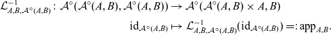 \begin{align*} \mathcal{L}_{A, B, \mathcal{A}^{\circ}(A, B)}^{-1} \colon \mathcal{A}^{\circ}(\mathcal{A}^{\circ}(A, B), \mathcal{A}^{\circ}(A, B)) & \to \mathcal{A}^{\circ}(\mathcal{A}^{\circ}(A, B) \times A, B) \\ \mathrm{id}_{\mathcal{A}^{\circ}(A, B)} & \mapsto \mathcal{L}_{A, B, \mathcal{A}^{\circ}(A, B)}^{-1}(\mathrm{id}_{\mathcal{A}^{\circ}(A, B)}) =: \mathrm{app}_{A,B}. \end{align*}
The arrow with the maps
 $\mathrm{app}_{A,B}$
are known as a higher-order arrow (Hughes, Reference Hughes2000), which is equivalent to an ordinary monad (i.e.
$\mathrm{app}_{A,B}$
are known as a higher-order arrow (Hughes, Reference Hughes2000), which is equivalent to an ordinary monad (i.e.
 $\mathcal{A}(A, B) = \mathbb{C}(A, \mathcal{T} B)$
for a monad
$\mathcal{A}(A, B) = \mathbb{C}(A, \mathcal{T} B)$
for a monad
 $\mathcal{T}$
).
$\mathcal{T}$
).
5.4 Soundness and adequacy
We prove the soundness (Theorem 5.13) of the operational semantics in Section 4.2 for the denotational semantics in Section 5.3.
First, observe the denotations of substituted terms and commands.
Lemma 5.11. The following hold.
-
1. If
$\Gamma, x : A \vdash M : B$
and
$\Gamma \vdash V : A$
, then
$\mathord{\left[\![{M[V / x]}\right]\!]}^S(c) = \mathord{\left[\![{M}\right]\!]}^S(c, \mathord{\left[\![{V}\right]\!]}^S(c))$
. -
2. If
and
$\Gamma \vdash V : A$
, then
$\mathord{\left[\![{P[V / x]}\right]\!]}^S(c) = \mathord{\left[\![{P}\right]\!]}^S(c, \mathord{\left[\![{V}\right]\!]}^S(c))$
. -
3. If
and
$\Gamma, \Delta \vdash V : A$
, then


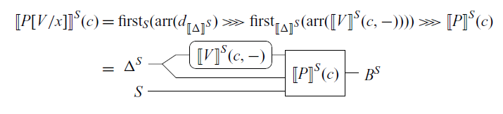
The following lemma is used to show the soundness for
 $(\mathop{\mathbf{handle}} \mathcal{F}[\mathsf{op}(V)] \mathop{\mathbf{with}} H) \to Q_{\mathsf{op}}[V / z, (\lambda^{\bullet} y : \delta . \mathop{\mathbf{handle}} \mathcal{F}[\lfloor{y}\rfloor] \mathop{\mathbf{with}} H) / k]$
.
$(\mathop{\mathbf{handle}} \mathcal{F}[\mathsf{op}(V)] \mathop{\mathbf{with}} H) \to Q_{\mathsf{op}}[V / z, (\lambda^{\bullet} y : \delta . \mathop{\mathbf{handle}} \mathcal{F}[\lfloor{y}\rfloor] \mathop{\mathbf{with}} H) / k]$
.
Lemma 5.12. If ![]() , then
, then
 \begin{equation*} \mathord{\left[\![{\mathcal{F}[\mathsf{op}(V)]}\right]\!]}^S(\star) = \mathop{\mathrm{first}}\nolimits_S(\mathop{\mathrm{arr}}\nolimits(\mathord{\left[\![{V}\right]\!]}^S) \mathrel{>\!\!>\!\!>} \mathsf{op}) \mathrel{>\!\!>\!\!>} \mathord{\left[\![{\mathcal{F}[\lfloor{y}\rfloor]}\right]\!]}^S(\star) \end{equation*}
holds.
Combining Lemmas 5.11 and 5.12, we obtain the soundness theorem for the arrow calculus with operations and handlers.
Theorem 5.13 (soundness). The following hold.
-
1. If
$\diamond \vdash M : A$
and
$M \to M'$
, then
$\mathord{\left[\![{M}\right]\!]}^S = \mathord{\left[\![{M'}\right]\!]}^S$
for any S. -
2. If
and
$P \to P'$
, then
$\mathord{\left[\![{P}\right]\!]}^S = \mathord{\left[\![{P'}\right]\!]}^S$
for any S.


Next, we prove the adequacy theorem using logical relations as done in Bauer and Pretnar (Reference Bauer and Pretnar2013), Sanada (Reference Sanada2023). The logical relations relate programs of type A and elements of
 $\mathord{\left[\![{A}\right]\!]}$
. Let
$\mathord{\left[\![{A}\right]\!]}$
. Let
 $\mathord{BType} = \{ \mathrm{Unit} \}$
. We add a constant
$\mathord{BType} = \{ \mathrm{Unit} \}$
. We add a constant
 $\mathtt{\langle\rangle}$
to the terms and values. We also add the following derivation rules to the arrow calculus:
$\mathtt{\langle\rangle}$
to the terms and values. We also add the following derivation rules to the arrow calculus:
The interpretation
 $\mathord{\left[\![{\mathrm{Unit}}\right]\!]}$
is the singleton set
$\mathord{\left[\![{\mathrm{Unit}}\right]\!]}$
is the singleton set
 $\{ \star \}$
and
$\{ \star \}$
and
 $\mathord{\left[\![{\mathtt{\langle\rangle}}\right]\!]}^S \colon \mathord{\left[\![{\Gamma}\right]\!]}^S \to \mathord{\left[\![{\mathrm{Unit}}\right]\!]}^S = \{ \star \}$
is the unique map.
$\mathord{\left[\![{\mathtt{\langle\rangle}}\right]\!]}^S \colon \mathord{\left[\![{\Gamma}\right]\!]}^S \to \mathord{\left[\![{\mathrm{Unit}}\right]\!]}^S = \{ \star \}$
is the unique map.
Definition 5.14 (logical relation). We define relations
 $(\triangleleft_A) \subseteq \mathord{\left[\![{A}\right]\!]} \times \{ M \mid \diamond \vdash M : A \} $
and
$(\triangleleft_A) \subseteq \mathord{\left[\![{A}\right]\!]} \times \{ M \mid \diamond \vdash M : A \} $
and ![]() for each type A as follows:
for each type A as follows:
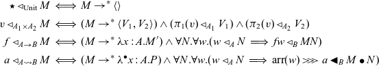 \begin{align*} \star \triangleleft_{\mathrm{Unit}} M & \iff M \to^* \mathtt{\langle\rangle} \\ v \triangleleft_{A_1 \times A_2} M & \iff (M \to^* \langle {V_1}, {V_2} \rangle) \land (\pi_1(v) \triangleleft_{A_1} V_1) \land (\pi_2(v) \triangleleft_{A_2} V_2) \\ f \triangleleft_{A \to B} M & \iff (M \to^* \lambda x : A . M') \land \forall N. \forall w. (w \triangleleft_A N \implies fw \triangleleft_B MN) \\ a \triangleleft_{A \rightsquigarrow B} M & \iff (M \to^* \lambda^{\bullet} x : A . P) \land \forall N. \forall w. (w \triangleleft_A N \implies \mathop{\mathrm{arr}}\nolimits(w) \mathrel{>\!\!>\!\!>} a \blacktriangleleft_B M \bullet N) \end{align*}
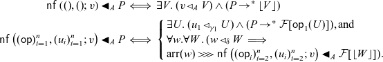 \begin{align*} \mathop{\mathsf{nf}}\left({()}, {()}; {v}\right) \blacktriangleleft_A P & \iff \exists V. \, (v \triangleleft_A V) \land (P \to^* \lfloor{V}\rfloor) \\ \mathop{\mathsf{nf}}\left({(\mathsf{op})_{i=1}^n}, {(u_i)_{i=1}^n}; {v}\right) \blacktriangleleft_A P & \iff \left\{ \begin{array}{l} \exists U . \, (u_1 \triangleleft_{\gamma_1} U) \land (P \to^* \mathcal{F}[\mathsf{op}_1(U)]), \text{and} \\ \forall w. \forall W.\, (w \triangleleft_{\delta} W \implies \\ \mathop{\mathrm{arr}}\nolimits(w) \mathrel{>\!\!>\!\!>} \mathop{\mathsf{nf}}\left({(\mathsf{op}_i)_{i=2}^n}, {(u_i)_{i=2}^n}; {v}\right) \blacktriangleleft_{A} \mathcal{F}[\lfloor{W}\rfloor]). \end{array} \right. \end{align*}
Note that by Proposition 5.5 every arrow term is equivalent to a normal form, and the relation
 $a \blacktriangleleft_A P$
is inductively defined on the number n of operations contained by an arrow term
$a \blacktriangleleft_A P$
is inductively defined on the number n of operations contained by an arrow term
 $a \in \mathcal{A}_{\Sigma}(1, \mathord{\left[\![{A}\right]\!]})$
.
$a \in \mathcal{A}_{\Sigma}(1, \mathord{\left[\![{A}\right]\!]})$
.
Lemma 5.15. The following hold.
-
1. If
$M \to^* M'$
and
$v \triangleleft_A M'$
, then
$v \triangleleft_A M$
. -
2. If
$M \to^* M'$
and
$v \triangleleft_A M$
, then
$v \triangleleft_A M'$
. -
3. If
$P \to^* P'$
and
$a \blacktriangleleft_A P'$
, then
$a \blacktriangleleft_A P$
. -
4. If
$P \to^* P'$
and
$a \blacktriangleleft_A P$
, then
$a \blacktriangleleft_A P'$
.


We can prove the following theorem using Lemma 5.15.
Theorem 5.16. Let
 $\Gamma = x_1 : A_1 , \dots , x_m : A_m$
and
$\Gamma = x_1 : A_1 , \dots , x_m : A_m$
and
 $\Delta = y_1 : B_1, \dots, y_n : B_n$
. The following hold.
$\Delta = y_1 : B_1, \dots, y_n : B_n$
. The following hold.
-
1. For
$\Gamma \vdash M : A$
and
$v_i \in \mathord{\left[\![{A_i}\right]\!]}$
and
$V_i$
with
$v_i \triangleleft_{A_i} V_i$
for each
$i \in \{ 1 , \dots , m\}$
,
\begin{equation*} \mathord{\left[\![{M}\right]\!]}(v_1, \dots, v_m) \triangleleft_A M[V_1 / x_1 , \dots, V_m / x_m]. \end{equation*}
-
2. For
,
$v_i \in \mathord{\left[\![{A_i}\right]\!]}$
and
$V_i$
with
$v_i \triangleleft_{A_i} V_i$
for each
$i \in \{ 1 , \dots , m\}$
and
$w_j \in \mathord{\left[\![{B_j}\right]\!]}$
and
$W_j$
with
$w_j \triangleleft_{B_j} W_j$
for each
$j \in \{ 1 , \dots , n\}$
,
\begin{align*} & \mathop{\mathrm{arr}}\nolimits(\langle w_1, \dots , w_n\rangle) \mathrel{>\!\!>\!\!>} \mathord{\left[\![{P}\right]\!]}(v_1, \dots, v_m) \\ & \blacktriangleleft_C P[V_1 / x_1 , \dots, V_m / x_m, W_1 / y_1, \dots , W_n / y_n]. \end{align*}


Proof sketch The proof is done by induction on the derivation of
 $\Gamma \vdash M : A$
and
$\Gamma \vdash M : A$
and ![]() .
.
Here, we only show the most non-trivial case ![]() , and the rest of the proof is sent to the appendix. The derivation is
, and the rest of the proof is sent to the appendix. The derivation is
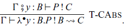
By the induction hypothesis, we have
 \begin{equation} \mathop{\mathrm{arr}}\nolimits(w) \mathrel{>\!\!>\!\!>} \mathord{\left[\![{P}\right]\!]}(v_1 , \dots, v_m) \blacktriangleleft_C P[V_1 / x_1 , \dots, V_m / x_m, W / y] \end{equation}
for any w and W with
 $w \triangleleft_B W$
. Given N and w satisfying
$w \triangleleft_B W$
. Given N and w satisfying
 $w \triangleleft_B N$
, we have
$w \triangleleft_B N$
, we have
 $N \to^* W$
for a value W by the definition of
$N \to^* W$
for a value W by the definition of
 $\triangleleft_B$
. Applying Lemma 5.15(2), we have
$\triangleleft_B$
. Applying Lemma 5.15(2), we have
 $w \triangleleft_B W$
. Hence, (5.14) holds for this w and W. Now, we have
$w \triangleleft_B W$
. Hence, (5.14) holds for this w and W. Now, we have
 \begin{align*} (\lambda^{\bullet} y : B. P[V_1 / x_1 , \dots, V_m / x_m]) \bullet N & \to^* (\lambda^{\bullet} y : B. P[V_1 / x_1 , \dots, V_m / x_m]) \bullet W \\ & \to P[V_1 / x_1 , \dots, V_m / x_m, W / y]. \end{align*}
Thus, applying Lemma 5.15(3), we have
 \begin{equation*} \mathop{\mathrm{arr}}\nolimits(w) \mathrel{>\!\!>\!\!>} \mathord{\left[\![{P}\right]\!]}(v_1 , \dots, v_m) \blacktriangleleft_C (\lambda^{\bullet} y : B. P[V_1 / x_1 , \dots, V_m / x_m]) \bullet N. \end{equation*}
Since
 $\mathord{\left[\![{P}\right]\!]} = \mathord{\left[\![{\lambda^{\bullet} y : B. P}\right]\!]}$
, we have
$\mathord{\left[\![{P}\right]\!]} = \mathord{\left[\![{\lambda^{\bullet} y : B. P}\right]\!]}$
, we have
 \begin{equation*} \mathord{\left[\![{\lambda^{\bullet} y : B. P}\right]\!]}(v_1, \dots, v_m) \triangleleft_{B \rightsquigarrow C} (\lambda^{\bullet} y : B. P[V_1 / x_1 , \dots, V_m / x_m]). \end{equation*}
corollary of the above theorem, we can show adequacy.
Corollary 5.17 (adequacy) If ![]() and
and
 $\mathord{\left[\![{P}\right]\!]} = \mathop{\mathrm{arr}}\nolimits(\star) \in \mathcal{A}_{\Sigma}(1, \mathord{\left[\![{\mathrm{Unit}}\right]\!]})$
, then
$\mathord{\left[\![{P}\right]\!]} = \mathop{\mathrm{arr}}\nolimits(\star) \in \mathcal{A}_{\Sigma}(1, \mathord{\left[\![{\mathrm{Unit}}\right]\!]})$
, then
 $P \to^* \lfloor{\mathtt{\langle\rangle}}\rfloor$
.
$P \to^* \lfloor{\mathtt{\langle\rangle}}\rfloor$
.
Proof By Theorem 5.16, we have
 $\mathop{\mathrm{arr}}\nolimits(\star) = \mathord{\left[\![{P}\right]\!]} \blacktriangleleft_{\mathrm{Unit}} P$
. By the definition of
$\mathop{\mathrm{arr}}\nolimits(\star) = \mathord{\left[\![{P}\right]\!]} \blacktriangleleft_{\mathrm{Unit}} P$
. By the definition of
 $\blacktriangleleft_{\mathrm{Unit}}$
, we have
$\blacktriangleleft_{\mathrm{Unit}}$
, we have
 $P \to^* \lfloor{V}\rfloor$
for a value V and
$P \to^* \lfloor{V}\rfloor$
for a value V and
 $\star \triangleleft_{\mathrm{Unit}} V$
. By the definition of
$\star \triangleleft_{\mathrm{Unit}} V$
. By the definition of
 $\triangleleft_{\mathrm{Unit}}$
, we have
$\triangleleft_{\mathrm{Unit}}$
, we have
 $V = \mathtt{\langle\rangle}$
. Hence,
$V = \mathtt{\langle\rangle}$
. Hence,
 $P \to^* \lfloor{\mathtt{\langle\rangle}}\rfloor$
.
$P \to^* \lfloor{\mathtt{\langle\rangle}}\rfloor$
.
6 Related work
Paterson (Reference Paterson2001) introduced a notation for arrows. As mentioned by Lindley et al. (Reference Lindley, Wadler and Yallop2010), there is a translation between the arrow calculus and Paterson’s notation, see Table 3.
Table 3. Translation between the arrow calculus and Paterson’s notation
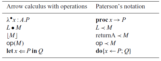
There is another approach to semantics for arrows: Freyd categories (Atkey, Reference Atkey2011). As Asada (Reference Asada2010, Theorem 23) proved, small strong monads on
 $\mathbb{C}$
in
$\mathbb{C}$
in ![]() with respect to the Yoneda embedding
with respect to the Yoneda embedding ![]() are equivalent to arrows in the sense of Atkey (Reference Atkey2011, Definition 2.1). We have adopted the profunctor approach because it is easier to consider with regard to algebras, which are the basis of handlers.
are equivalent to arrows in the sense of Atkey (Reference Atkey2011, Definition 2.1). We have adopted the profunctor approach because it is easier to consider with regard to algebras, which are the basis of handlers.
T There are some notions of algebras for arrows or profunctors. Jacobs et al. (Reference Jacobs, Heunen and Hasuo2009) defined an algebra for a promonad ![]() as a 2-cell
as a 2-cell
 $\chi \colon \mathcal{A} \Rightarrow \mathrm{I}_{\mathbb{C}}$
subject to some axioms (Jacobs et al., Reference Jacobs, Heunen and Hasuo2009, Definition 6.5), which is different from ours. From a 2-cell
$\chi \colon \mathcal{A} \Rightarrow \mathrm{I}_{\mathbb{C}}$
subject to some axioms (Jacobs et al., Reference Jacobs, Heunen and Hasuo2009, Definition 6.5), which is different from ours. From a 2-cell
 $\chi \colon \mathcal{A} \Rightarrow \mathrm{I}_{\mathbb{C}}$
, we obtain
$\chi \colon \mathcal{A} \Rightarrow \mathrm{I}_{\mathbb{C}}$
, we obtain
 $\mathcal{A} \circ \mathbb{C}({-}, C) \Rightarrow \mathbb{C}({-}, C)$
for any
$\mathcal{A} \circ \mathbb{C}({-}, C) \Rightarrow \mathbb{C}({-}, C)$
for any
 $C \in \mathrm{Ob}(\mathbb{C})$
. Hence, an algebra in the sense of Jacobs et al. (Reference Jacobs, Heunen and Hasuo2009) is a family of special algebras in this paper.
$C \in \mathrm{Ob}(\mathbb{C})$
. Hence, an algebra in the sense of Jacobs et al. (Reference Jacobs, Heunen and Hasuo2009) is a family of special algebras in this paper.
In nLab (2021), an algebra for a profunctor ![]() is defined as a pair (X, x) of an object
is defined as a pair (X, x) of an object
 $X \in \mathbb{C}$
and an element
$X \in \mathbb{C}$
and an element
 $x \in H(X,X)$
, which does not induce our definition of algebras.
$x \in H(X,X)$
, which does not induce our definition of algebras.
Altenkirch et al. (Reference Altenkirch, Chapman and Uustalu2010) introduced relative monads as a generalisation of monads. Let
 $\mathbb{C}$
be a category and
$\mathbb{C}$
be a category and
 $\widehat{{\mathbb{C}}} = [\mathbb{C}^{\mathrm{op}}, \mathbf{Set}]$
. A relative monad
$\widehat{{\mathbb{C}}} = [\mathbb{C}^{\mathrm{op}}, \mathbf{Set}]$
. A relative monad
 ${\mathcal{T}} \colon \mathbb{C} \to \widehat{{\mathbb{C}}}$
on the Yoneda embedding
${\mathcal{T}} \colon \mathbb{C} \to \widehat{{\mathbb{C}}}$
on the Yoneda embedding ![]() corresponds to a promonad on
corresponds to a promonad on
 $\mathbb{C}$
(Altenkirch et al., Reference Altenkirch, Chapman and Uustalu2010, Theorem 9). An Eilenberg–Moore algebra for
$\mathbb{C}$
(Altenkirch et al., Reference Altenkirch, Chapman and Uustalu2010, Theorem 9). An Eilenberg–Moore algebra for
 ${\mathcal{T}}$
is a pair
${\mathcal{T}}$
is a pair
 $(G, \chi)$
of an object
$(G, \chi)$
of an object
 $G \in \widehat{{\mathbb{C}}}$
and a natural transformation
$G \in \widehat{{\mathbb{C}}}$
and a natural transformation ![]() subject to some axioms (Altenkirch et al., Reference Altenkirch, Chapman and Uustalu2010, Definition 3). Eilenberg–Moore algebras for a relative monad
subject to some axioms (Altenkirch et al., Reference Altenkirch, Chapman and Uustalu2010, Definition 3). Eilenberg–Moore algebras for a relative monad
 ${\mathcal{T}}$
are equivalent to algebras in the sense of Definition 3.1 for the promonad
${\mathcal{T}}$
are equivalent to algebras in the sense of Definition 3.1 for the promonad
 $\mathcal{A}$
defined by
$\mathcal{A}$
defined by
 $\mathcal{A}(X,Y) = {\mathcal{T}} YX$
. Especially, giving
$\mathcal{A}(X,Y) = {\mathcal{T}} YX$
. Especially, giving ![]() natural in Z is equivalent to giving
natural in Z is equivalent to giving
 $\alpha \colon \mathcal{A}(Y,Z) \times GY \to GZ$
natural in Z and extranatural in Y because we have
$\alpha \colon \mathcal{A}(Y,Z) \times GY \to GZ$
natural in Z and extranatural in Y because we have
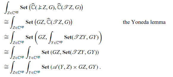
Here, we used end
 $\int_{X} ({-})$
, which is the dual notion of coend. Uustalu (Reference Uustalu2010) introduced strong relative monads, which corresponds to strong promonads.
$\int_{X} ({-})$
, which is the dual notion of coend. Uustalu (Reference Uustalu2010) introduced strong relative monads, which corresponds to strong promonads.
Pieters et al. (Reference Pieters, Rivas and Schrijvers2020) introduced handlers for monoidal effects. In their framework, an inductive handler for arrows (without static parameters) is constructed by giving a 2-cell
 $(\mathrm{I}_{\mathbb{C}} + \vec{\Sigma} \circ \mathcal{A}) \Rightarrow \mathcal{A}$
in the bicategory of (strong) profunctors, where
$(\mathrm{I}_{\mathbb{C}} + \vec{\Sigma} \circ \mathcal{A}) \Rightarrow \mathcal{A}$
in the bicategory of (strong) profunctors, where ![]() . A 2-cell
. A 2-cell
 $(\mathrm{I}_{\mathbb{C}} + \vec{\Sigma} \circ \mathcal{A}) \Rightarrow \mathcal{A}$
consists of
$(\mathrm{I}_{\mathbb{C}} + \vec{\Sigma} \circ \mathcal{A}) \Rightarrow \mathcal{A}$
consists of
-
• a family of maps
$\eta_{A,B} \colon \mathbb{C}(A,B) \to \mathcal{A}(A,B)$
natural in A and B, and -
• families of maps
$\iota_{\mathrm{op},A,B,C} \colon \mathbb{C}(A,\mathord{\left[\![{\gamma}\right]\!]} \times (\mathord{\left[\![{\delta}\right]\!]}\Rightarrow C)) \times \mathcal{A}(C, B) \to \mathcal{A}(A,B)$
natural in A and B and extranatural in C.


From this semantic structure, Pieters et al. (Reference Pieters, Rivas and Schrijvers2020) defined syntax of inductive handlers for arrows (without static parameters) as follows.
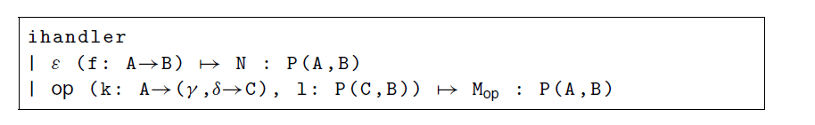
From an inductive handler, we can obtain a handler in the sense of this paper because we have the following map in
 $\mathbf{Set}$
:
$\mathbf{Set}$
:
Proposition 6.1. There is a map
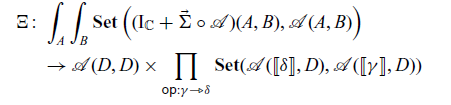
for any set D.
Hence, given a 2-cell
 $h \colon (\mathrm{I}_{\mathbb{C}} + \vec{\Sigma} \circ \mathcal{A}) \Rightarrow \mathcal{A}$
, we have
$h \colon (\mathrm{I}_{\mathbb{C}} + \vec{\Sigma} \circ \mathcal{A}) \Rightarrow \mathcal{A}$
, we have
 $\pi_1(\Xi(h)) \in \mathcal{A}(D,D)$
and
$\pi_1(\Xi(h)) \in \mathcal{A}(D,D)$
and
 $\{ \pi_{\mathsf{op}}(\pi_2(\Xi(h))) \colon \mathcal{A}(\mathord{\left[\![{\delta}\right]\!]}, D) \to \mathcal{A}(\mathord{\left[\![{\gamma}\right]\!]}, D)\}_{\mathsf{op}}$
, which determine a handler in the sense of this paper. Note that inductive handlers cannot modify the answer type whereas handlers in the sense of this paper can.
$\{ \pi_{\mathsf{op}}(\pi_2(\Xi(h))) \colon \mathcal{A}(\mathord{\left[\![{\delta}\right]\!]}, D) \to \mathcal{A}(\mathord{\left[\![{\gamma}\right]\!]}, D)\}_{\mathsf{op}}$
, which determine a handler in the sense of this paper. Note that inductive handlers cannot modify the answer type whereas handlers in the sense of this paper can.
7 Conclusion and future work
We have introduced an arrow calculus with operations and handlers and defined its operational semantics and denotational semantics. The calculus design is based on categorical observations. The preservation and progress theorems are proved. We have also proved soundness and adequacy.
For future work, we plan to investigate the following topics.
 $\lambda_{\mathrm{flow}}$
is a calculus with handlers for monads, arrows and idioms (Lindley, Reference Lindley2014). The relationship between the arrow calculus with operations and handlers and
$\lambda_{\mathrm{flow}}$
is a calculus with handlers for monads, arrows and idioms (Lindley, Reference Lindley2014). The relationship between the arrow calculus with operations and handlers and
 $\lambda_{\mathrm{flow}}$
is to be investigated. Is there translation from the arrow calculus with operations and handlers to Lindley’s
$\lambda_{\mathrm{flow}}$
is to be investigated. Is there translation from the arrow calculus with operations and handlers to Lindley’s
 $\lambda_{\mathrm{flow}}$
?
$\lambda_{\mathrm{flow}}$
?
Combination of handlers for monads and arrows in categorical way is interesting to investigate. Monoidal effects by Pieters et al. (Reference Pieters, Rivas and Schrijvers2020) are one answer to this question. As another answer, can we use double categorical frameworks, focusing on the relationship between monads and promonads?
An algebraic theory corresponds to a finitary monad (Adamek and Rosicky, Reference Adamek and Rosicky1994). Can we develop a promonad version of such theory?
Acknowledgements
We thank Kazuyuki Asada for helpful discussions, suggestions on the structure of the paper and comments, Masahito Hasegawa, Ichiro Hasuo, Satoshi Kura, Keisuke Hoshino and Yuto Kawase for helpful discussions and comments and anonymous reviewers for their many valuable suggestions, comments and pointing us to related work. We also thank Soichiro Fujii for providing his gentle introduction to profunctors (Fujii Reference Fujii2021). This work was supported by JST Grant Number JPMJFS2123.
Conflicts of interest
None.
A Coends
In this section, we review the definition and construction of coends. We also give an informal description of coends.
Definition A.1. (extranatural transformation). Let
 $F, G \colon \mathbb{C}^{\mathrm{op}} \times \mathbb{C} \to \mathbb{D}$
be functors. An extranatural transformation
$F, G \colon \mathbb{C}^{\mathrm{op}} \times \mathbb{C} \to \mathbb{D}$
be functors. An extranatural transformation
 $\phi$
from F to G, we write
$\phi$
from F to G, we write
 $\phi \colon F \Rightarrow G$
, is a family of morphisms
$\phi \colon F \Rightarrow G$
, is a family of morphisms
 $ (\phi_C \colon F(C, C) \to G(C, C))_{C \in \mathrm{Ob}(\mathbb{C})} $
such that the following diagram commutes for any morphisms
$ (\phi_C \colon F(C, C) \to G(C, C))_{C \in \mathrm{Ob}(\mathbb{C})} $
such that the following diagram commutes for any morphisms
 $f \colon C \to C'$
in
$f \colon C \to C'$
in
 $\mathbb{C}$
:
$\mathbb{C}$
:
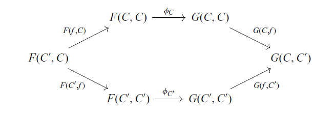
In the following, we deal only with extranatural transformations whose codomain (G) is a constant functor.
A coend is a pair of an object and an extranatural transformation defined for a functor. It has a universal property like a colimit.
Definition 1.2 (coend). Let
 $F \colon \mathbb{C}^{\mathrm{op}} \times \mathbb{C} \to \mathbb{D}$
be a functor. A coend of F is a pair of an object
$F \colon \mathbb{C}^{\mathrm{op}} \times \mathbb{C} \to \mathbb{D}$
be a functor. A coend of F is a pair of an object
 $\int^{C \in \mathbb{C}} F(C, C) \in \mathbb{D}$
and an extranatural transformation
$\int^{C \in \mathbb{C}} F(C, C) \in \mathbb{D}$
and an extranatural transformation
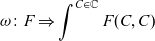 \begin{equation*} \omega \colon F \Rightarrow \int^{C \in \mathbb{C}} F(C, C) \end{equation*}
satisfying the following universal property. If
 $\phi \colon F \Rightarrow X$
is an extranatural transformation to an object
$\phi \colon F \Rightarrow X$
is an extranatural transformation to an object
 $X \in \mathbb{D}$
, then there exists a unique morphism
$X \in \mathbb{D}$
, then there exists a unique morphism
 $\kappa \colon \int^{C \in \mathbb{C}} F(C, C) \to X$
such that
$\kappa \colon \int^{C \in \mathbb{C}} F(C, C) \to X$
such that
 $\phi = \kappa \circ \omega$
:
$\phi = \kappa \circ \omega$
:
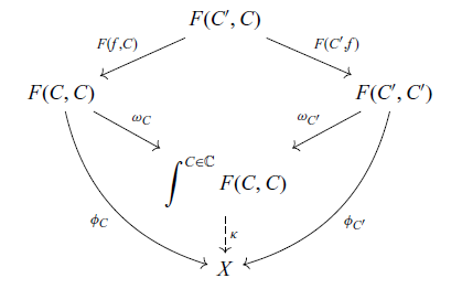
The existence of a coend of
 $F \colon \mathbb{C}^{\mathrm{op}} \times \mathbb{C} \to \mathbb{D}$
depends on the properties of
$F \colon \mathbb{C}^{\mathrm{op}} \times \mathbb{C} \to \mathbb{D}$
depends on the properties of
 $\mathbb{C}$
,
$\mathbb{C}$
,
 $\mathbb{D}$
and F. The following proposition is known (Loregian, Reference Loregian2021, (1.29)) for the cases we often use in this paper.
$\mathbb{D}$
and F. The following proposition is known (Loregian, Reference Loregian2021, (1.29)) for the cases we often use in this paper.
Proposition A.3. If
 $\mathbb{C}$
is small, for the functor
$\mathbb{C}$
is small, for the functor
 $F \colon \mathbb{C}^{\mathrm{op}} \times \mathbb{C} \to \mathbf{Set}$
, the coend
$F \colon \mathbb{C}^{\mathrm{op}} \times \mathbb{C} \to \mathbf{Set}$
, the coend
 $\omega \colon F \Rightarrow \int^{C \in \mathbb{C}} F(C, C)$
of F always exists.
$\omega \colon F \Rightarrow \int^{C \in \mathbb{C}} F(C, C)$
of F always exists.
Proof We only construct the set
 $\int^{C \in \mathbb{C}} F(C, C)$
and
$\int^{C \in \mathbb{C}} F(C, C)$
and
 $\omega$
, and the proof of universality is left to the reader. First, we define an equivalence relation
$\omega$
, and the proof of universality is left to the reader. First, we define an equivalence relation
 $\sim$
on a set
$\sim$
on a set
 $\coprod_{C \in \mathrm{Ob}(\mathbb{C})} F(C,C)$
as follows. For
$\coprod_{C \in \mathrm{Ob}(\mathbb{C})} F(C,C)$
as follows. For
 $a \in F(C,C)$
and
$a \in F(C,C)$
and
 $b \in F(C', C')$
,
$b \in F(C', C')$
,
 $a \sim b$
if there exists a morphism
$a \sim b$
if there exists a morphism
 $f \colon C \to C'$
in
$f \colon C \to C'$
in
 $\mathbb{C}$
and
$\mathbb{C}$
and
 $c \in F(C', C)$
such that
$c \in F(C', C)$
such that
 $F(f, C)(c) = a$
and
$F(f, C)(c) = a$
and
 $F(C', f)(c) = b$
.
$F(C', f)(c) = b$
.
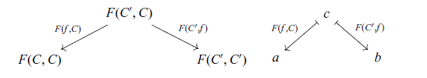
We write [a] for the equivalence class of
 $a \in F(C,C)$
in
$a \in F(C,C)$
in
 $\sim$
. Now, we define
$\sim$
. Now, we define
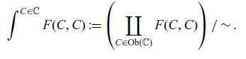 \begin{equation} \int^{C \in \mathbb{C}} F(C, C) :=\left(\coprod_{C \in \mathrm{Ob}(\mathbb{C})} F(C,C) \right)/ \sim. \end{equation}
We define
 $\omega_C \colon F(C,C) \to \int^{C \in \mathbb{C}} F(C, C)$
as the canonical injection:
$\omega_C \colon F(C,C) \to \int^{C \in \mathbb{C}} F(C, C)$
as the canonical injection:
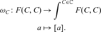 \begin{equation*} \begin{split} \omega_C \colon F(C,C) & \to \int^{C \in \mathbb{C}} F(C, C) \\ a & \mapsto [a]. \end{split} \end{equation*}
The proof of Proposition A.3 relies on the construction (A1), which small cocompleteness of
 $\mathbf{Set}$
. Similarly, we can show that a coend
$\mathbf{Set}$
. Similarly, we can show that a coend
 $\int^C F(C,C)$
for a functor
$\int^C F(C,C)$
for a functor
 $F \colon \mathbf{Set}^{\mathrm{op}} \times \mathbf{Set} \to \mathbf{Ens}$
exists because
$F \colon \mathbf{Set}^{\mathrm{op}} \times \mathbf{Set} \to \mathbf{Ens}$
exists because
 $\mathbf{Ens}$
is sufficiently cocomplete.
$\mathbf{Ens}$
is sufficiently cocomplete.
Informally, we can think of
 $\int^{C \in \mathbb{C}}$
as an existential quantifier
$\int^{C \in \mathbb{C}}$
as an existential quantifier
 $\exists$
over
$\exists$
over
 $C \in \mathrm{Ob}(\mathbb{C})$
. An element w of
$C \in \mathrm{Ob}(\mathbb{C})$
. An element w of
 $\int^{C \in \mathbb{C}} F(C, C)$
is regarded as a witness of a proposition that there exists
$\int^{C \in \mathbb{C}} F(C, C)$
is regarded as a witness of a proposition that there exists
 $C \in \mathrm{Ob}(\mathbb{C})$
such that F(C, C) holds.
$C \in \mathrm{Ob}(\mathbb{C})$
such that F(C, C) holds.
B 2-Categories, bicategories and enriched categories
B.1 2-Categories
Roughly speaking, a 2-category is a category whose hom-sets have a categorical structure.
Definition B.1 (2-categories). A 2-category
 $\mathbf{C}$
consists of the following data.
$\mathbf{C}$
consists of the following data.
-
• A class
$\mathrm{Ob}(\mathbf{C})$
. We call an element a of
$\mathrm{Ob}(\mathbf{C})$
an object or a 0-cell. -
• A family
$\{ \mathbf{C}(a, b) \}_{a, b \in \mathrm{Ob}(\mathbf{C})}$
of categories, called hom-categories. We call an object f of
$\mathbf{C}(a, b)$
a morphism or a 1-cell from a to b of
$\mathbf{C}$
. A morphism
$\alpha \colon f \to g$
in
$\mathbf{C}(a, b)$
is called a 2-cell from f to g of
$\mathbf{C}$
. -
• An identity functor
$\mathrm{id}_a \colon \mathbf{1} \to \mathbf{C}(a,a)$
for each
$a \in \mathrm{Ob}(\mathbf{C})$
. -
• A composition functor
for each
$a, b, c \in \mathrm{Ob}(\mathbf{C})$


subject to the following axioms expressed by the (strict) commutativity of
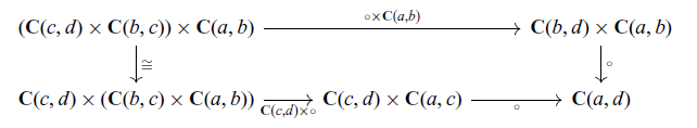
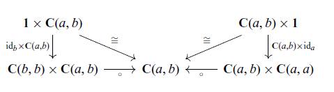
We write
 $f \colon a \to b$
for a 1-cell f from a to b, and
$f \colon a \to b$
for a 1-cell f from a to b, and
 $\alpha \colon f \Rightarrow g$
for a 2-cell
$\alpha \colon f \Rightarrow g$
for a 2-cell
 $\alpha$
from f to g:
$\alpha$
from f to g:
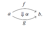
We also write
 $g \circ f$
for the composition
$g \circ f$
for the composition ![]() of 1-cells
of 1-cells
 $f \colon a \to b$
and
$f \colon a \to b$
and
 $g \colon b \to c$
.
$g \colon b \to c$
.
For 1-cells, the axiom (B1) is the associativity of composition and (B2) is the unitality of composition. Let
 $f \colon a \to b$
,
$f \colon a \to b$
,
 $g \colon b \to c$
and
$g \colon b \to c$
and
 $h \colon c \to d$
be 1-cells in a 2-category
$h \colon c \to d$
be 1-cells in a 2-category
 $\mathbf{C}$
. The associativity of composition (B1) for the 1-cells f, g and h is
$\mathbf{C}$
. The associativity of composition (B1) for the 1-cells f, g and h is
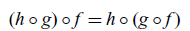 \begin{equation} (h \circ g) \circ f = h \circ (g \circ f)\end{equation}
in the hom-category
 $\mathbf{C}(a,d)$
, and the unitality (B2) for the 1-cell f is
$\mathbf{C}(a,d)$
, and the unitality (B2) for the 1-cell f is
 \begin{equation} (\mathrm{id}_b \circ f) = f = (f \circ \mathrm{id}_a)\end{equation}
in the hom-category
 $\mathbf{C}(a,b)$
.
$\mathbf{C}(a,b)$
.
An example of 2-categories is the 2-category
 $\mathbf{Cat}$
, whose 0-cells, 1-cells and 2-cells are small categories, functors and natural transformation, respectively.
$\mathbf{Cat}$
, whose 0-cells, 1-cells and 2-cells are small categories, functors and natural transformation, respectively.
2-category theory is a formal language to describe the ordinary category theory. For example, a definition of monads in 2-categories is as follows.
Definition B.2 (monads in 2-categories). Let
 $\mathbf{C}$
be a 2-category. A monad in
$\mathbf{C}$
be a 2-category. A monad in
 $\mathbf{C}$
is an endo 1-cell
$\mathbf{C}$
is an endo 1-cell
 $t \colon c \to c$
equipped with
$t \colon c \to c$
equipped with
-
• a 2-cell
$\eta \colon \mathrm{id}_c \Rightarrow t$
called a unit and -
• a 2-cell
$\mu \colon t \circ t \Rightarrow t$
called a multiplication


such that the following axioms hold:
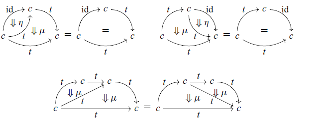
Monads in the 2-category
 $\mathbf{Cat}$
in the sense of Definition B.2 coincide with ordinary monads.
$\mathbf{Cat}$
in the sense of Definition B.2 coincide with ordinary monads.
B.2 Bicategories
In the definition of 2-categories, the axioms (B1) and (B2) are strict in the sense that the equalities hold in the hom-categories. From a category-theoretic principle, these axioms may be too strict because we want to identify two functors in (B1) and (B2) which are not only strictly equal, but naturally isomorphic.
Definition B.3 (bicategories). A bicategory
 $\mathbf{C}$
consists of the same data in the definition of 2-categories (Definition B.1) which make (B1) and (B2) commute up to natural isomorphism.
$\mathbf{C}$
consists of the same data in the definition of 2-categories (Definition B.1) which make (B1) and (B2) commute up to natural isomorphism.
For 1-cells
 $f \colon a \to b$
,
$f \colon a \to b$
,
 $g \colon b \to c$
and
$g \colon b \to c$
and
 $h \colon c \to d$
in a bicategory
$h \colon c \to d$
in a bicategory
 $\mathbf{C}$
, the associativity of composition (B1) and the unitality (B2) are expressed as follows:
$\mathbf{C}$
, the associativity of composition (B1) and the unitality (B2) are expressed as follows:
 \begin{align} (h \circ g) \circ f \cong h \circ (g \circ f) & & \text{in the category $\mathbf{C}(a, d)$,}\end{align}
 \begin{align}(\mathrm{id}_b \circ f) \cong f \cong (f \circ \mathrm{id}_a)& & \text{in the category $\mathbf{C}(a,b)$.}\end{align}
The equalities in (B3) and (B4) are replaced by the isomorphisms.
We can obtain a definition of monads in bicategories from the definition of monads in 2-categories (Definition B.2).
B.3 Enriched categories
We write
 $\mathbf{Cat}_0 = (\mathbf{Cat}_0, \times, \mathbf{1})$
for the monoidal category of small categories and functors. In the definition of 2-categories (Definition B.1), the monoidal structure of
$\mathbf{Cat}_0 = (\mathbf{Cat}_0, \times, \mathbf{1})$
for the monoidal category of small categories and functors. In the definition of 2-categories (Definition B.1), the monoidal structure of
 $\mathbf{Cat}_0$
is essential to describe the identity functors
$\mathbf{Cat}_0$
is essential to describe the identity functors
 $\mathrm{id}_a$
and composition functors
$\mathrm{id}_a$
and composition functors ![]() and the axioms. The descriptions of the identity and composition in ordinary categories also use the monoidal structure of
and the axioms. The descriptions of the identity and composition in ordinary categories also use the monoidal structure of
 $\mathbf{Set} = (\mathbf{Set}, \times, 1)$
. We generalise (2-)categories from this perspective and obtain the following definition of enriched categories.
$\mathbf{Set} = (\mathbf{Set}, \times, 1)$
. We generalise (2-)categories from this perspective and obtain the following definition of enriched categories.
Definition B.4 (enriched category). Let
 $\mathbb{V} = (\mathbb{V}, \otimes, J)$
be a symmetric monoidal category. A
$\mathbb{V} = (\mathbb{V}, \otimes, J)$
be a symmetric monoidal category. A
 $\mathbb{V}$
-enriched category (or simply a
$\mathbb{V}$
-enriched category (or simply a
 $\mathbb{V}$
-category)
$\mathbb{V}$
-category)
 $\mathbb{C}$
consists of the following data.
$\mathbb{C}$
consists of the following data.
-
• A class
$\mathrm{Ob}(\mathbb{C})$
of objects. -
• A family of objects
$\{ \mathbb{C}(a,b) \}_{a, b \in \mathrm{Ob}(\mathbb{C})}$
of
$\mathbb{V}$
. We call
$\mathbb{C}(a,b) \in \mathbb{V}$
a hom-object. -
• A morphism
$\mathrm{id}_a \colon J \to \mathbb{C}(a,a)$
for each
$a \in \mathrm{Ob}(\mathbb{C})$
, called an identity. -
• A morphism
for each
$a, b, c \in \mathrm{Ob}(\mathbb{C})$
, called a composition


subject to the following axioms expressed by the commutativity of
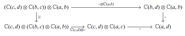
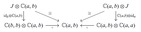
An ordinary category is a
 $\mathbf{Set}$
-enriched category, and a 2-category in the sense of Definition B.1 is a
$\mathbf{Set}$
-enriched category, and a 2-category in the sense of Definition B.1 is a
 $\mathbf{Cat}_0$
-enriched category.
$\mathbf{Cat}_0$
-enriched category.
The enriched version of a functor between categories is called a
 $\mathbb{V}$
-functor, which preserves
$\mathbb{V}$
-functor, which preserves
 $\mathbb{V}$
-category structures. See Kelly (Reference Kelly1982) for the definition.
$\mathbb{V}$
-category structures. See Kelly (Reference Kelly1982) for the definition.
C Proofs for Section 4 (The arrow calculus with operations and handlers)
Proposition 4.1 (progress). The following hold.
-
1. For any well-typed term
$\diamond \vdash M : A$
, there exists a term M’ such that
$M \to M'$
or M is a value. -
2. For any well-typed command
, one of following holds.-
a. There exists a command P’ such that
$P \to P'$
. -
b. <texmath>inline504</texmath> for some value V.
-
c.
$P = \mathcal{F}{[\mathsf{op}(V)]}$
for some operation
$\mathsf{op}$
, value V and context
$\mathcal{F}$
.
-


Proof. (1). By induction on the derivation of
 $\diamond \vdash M : A$
.
$\diamond \vdash M : A$
.
In case ![]() . This case cannot happen because the context is empty.
. This case cannot happen because the context is empty.
In case ![]() . In this case, we have
. In this case, we have
 $M = \lambda x . N$
for some term N, and M is a value.
$M = \lambda x . N$
for some term N, and M is a value.
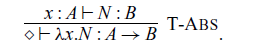
In case ![]() . We have
. We have
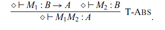
By the induction hypothesis,
 $M_1$
is a value or
$M_1$
is a value or
 $M_1 \to M_1'$
for some
$M_1 \to M_1'$
for some
 $M_1'$
, and
$M_1'$
, and
 $M_2$
is a value or
$M_2$
is a value or
 $M_2 \to M_2'$
for some
$M_2 \to M_2'$
for some
 $M_2'$
. If
$M_2'$
. If
 $M_1 \to M_1'$
holds for some
$M_1 \to M_1'$
holds for some
 $M_1'$
, then we have
$M_1'$
, then we have
 $M_1 M_2 \to M_1' M_2$
. If
$M_1 M_2 \to M_1' M_2$
. If
 $M_1$
is a value, then
$M_1$
is a value, then
 $M_1 = \lambda x . N$
for some N because
$M_1 = \lambda x . N$
for some N because
 $\diamond \vdash M_1 : A \to B$
. We have two subcases: If
$\diamond \vdash M_1 : A \to B$
. We have two subcases: If
 $M_2$
is a value V, then we have
$M_2$
is a value V, then we have
 $M_1 M_2 = (\lambda x . N) V \to N[V / x]$
. If
$M_1 M_2 = (\lambda x . N) V \to N[V / x]$
. If
 $M_2 \to M_2'$
holds for some
$M_2 \to M_2'$
holds for some
 $M_2'$
, then we have
$M_2'$
, then we have
 $M_1 M_2 = (\lambda x . N) M_2 \to (\lambda x . N) M_2'$
.
$M_1 M_2 = (\lambda x . N) M_2 \to (\lambda x . N) M_2'$
.
In case ![]() . In this case, we have
. In this case, we have
 $M = \lambda^{\bullet} x . N$
for some term N, and M is a value.
$M = \lambda^{\bullet} x . N$
for some term N, and M is a value.
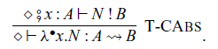
In case ![]() .
.
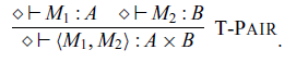
By the induction hypothesis,
 $M_1$
is a value or
$M_1$
is a value or
 $M_1 \to M_1'$
for some
$M_1 \to M_1'$
for some
 $M_1'$
, and
$M_1'$
, and
 $M_2$
is a value or
$M_2$
is a value or
 $M_2 \to M_2'$
for some
$M_2 \to M_2'$
for some
 $M_2'$
. If
$M_2'$
. If
 $M_1 \to M_1'$
holds for some
$M_1 \to M_1'$
holds for some
 $M_1'$
, then we have
$M_1'$
, then we have
 $\langle {M_1}, {M_2} \rangle \to \langle {M_1'}, {M_2} \rangle$
. If
$\langle {M_1}, {M_2} \rangle \to \langle {M_1'}, {M_2} \rangle$
. If
 $M_1$
is a value
$M_1$
is a value
 $V_1$
, we have two subcases: if
$V_1$
, we have two subcases: if
 $M_2$
is a value
$M_2$
is a value
 $V_2$
, then
$V_2$
, then
 $M = \langle {M_1}, {M_2} \rangle = \langle {V_1}, {V_2} \rangle$
is a value. If
$M = \langle {M_1}, {M_2} \rangle = \langle {V_1}, {V_2} \rangle$
is a value. If
 $M_2 \to M_2'$
holds for some
$M_2 \to M_2'$
holds for some
 $M_2'$
, then we have
$M_2'$
, then we have
 $\langle {M_1}, {M_2} \rangle = \langle {V_1}, {M_2} \rangle \to \langle {V_1}, {M_2'} \rangle$
.
$\langle {M_1}, {M_2} \rangle = \langle {V_1}, {M_2} \rangle \to \langle {V_1}, {M_2'} \rangle$
.
In case ![]() ,
, ![]() . Straightforward.
. Straightforward.
(2). By induction on the derivation of ![]() .
.
In case ![]() . We have
. We have
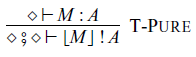
for some term M. By (1), M is a value or
 $M \to M'$
holds for some M’. If M is a value V, then
$M \to M'$
holds for some M’. If M is a value V, then
 $P = \lfloor{V}\rfloor$
and this satisfies (b). If
$P = \lfloor{V}\rfloor$
and this satisfies (b). If
 $M \to M'$
holds for some M’, then we have
$M \to M'$
holds for some M’, then we have
 $P = \lfloor{M}\rfloor \to \lfloor{M'}\rfloor$
.
$P = \lfloor{M}\rfloor \to \lfloor{M'}\rfloor$
.
In case ![]() . We have
. We have
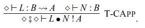
By the similar argument to Case T
-App, we have either
 $L \bullet N \to L' \bullet N$
for some L’,
$L \bullet N \to L' \bullet N$
for some L’,
 $L = (\lambda^{\bullet} x. L_1)$
and
$L = (\lambda^{\bullet} x. L_1)$
and
 $L \bullet N \to L \bullet N'$
for some N’, or
$L \bullet N \to L \bullet N'$
for some N’, or
 $L = (\lambda^{\bullet} x. L_1)$
, N is a value, and
$L = (\lambda^{\bullet} x. L_1)$
, N is a value, and
 $L \bullet N = (\lambda^{\bullet} x. L_1) \bullet V \to L_1[V/x]$
for some V.
$L \bullet N = (\lambda^{\bullet} x. L_1) \bullet V \to L_1[V/x]$
for some V.
In case ![]() . We have
. We have
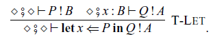
By the induction hypothesis, we have the following three cases.
-
1.
$P \to P'$
for some command P’. We have
$(\mathop{\mathbf{let}} x \Leftarrow P \mathop{\mathbf{in}} Q) \to (\mathop{\mathbf{let}} x \Leftarrow P' \mathop{\mathbf{in}} Q)$
. -
2.
$P = \lfloor{V}\rfloor$
for some value term V. We have
$(\mathop{\mathbf{let}} x \Leftarrow P \mathop{\mathbf{in}} Q) = (\mathop{\mathbf{let}} x \Leftarrow \lfloor{V}\rfloor \mathop{\mathbf{in}} Q) \to Q[V / x]$
. -
3.
$P = \mathcal{F}[\mathsf{op}(V)]$
for some value term V, operation symbol
$\mathsf{op} \in \Sigma$
and context
$\mathcal{F}$
. We have
$P = \mathcal{F}'[\mathsf{op}(V)]$
for
$\mathcal{F}' = (\mathop{\mathbf{let}} x \Leftarrow \mathcal{F} \mathop{\mathbf{in}} Q)$
.


In case ![]() . We have
. We have
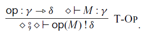
By the induction hypothesis, M is a value or
 $M \to M'$
for some M’. If M is a value V, then
$M \to M'$
for some M’. If M is a value V, then
 $P = \mathsf{op}(V) = \mathcal{F}[\mathsf{op}(V)]$
for
$P = \mathsf{op}(V) = \mathcal{F}[\mathsf{op}(V)]$
for
 $\mathcal{F} = [{-}]$
. If
$\mathcal{F} = [{-}]$
. If
 $M \to M'$
holds, then
$M \to M'$
holds, then
 $P = \mathsf{op}(M) \to \mathsf{op}(M')$
.
$P = \mathsf{op}(M) \to \mathsf{op}(M')$
.
In case ![]() . We have
. We have
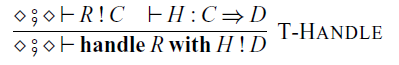
where ![]() . By the induction hypothesis, we have the following three cases.
. By the induction hypothesis, we have the following three cases.
-
1.
$R \to R'$
for some command R’. We have
$(\mathop{\mathbf{handle}} R \mathop{\mathbf{with}} H) \to (\mathop{\mathbf{handle}} R' \mathop{\mathbf{with}} H)$
. -
2.
$R = \lfloor{V}\rfloor$
for some value term V. We have
\[ (\mathop{\mathbf{handle}} R \mathop{\mathbf{with}} H) = (\mathop{\mathbf{handle}} \lfloor{V}\rfloor \mathop{\mathbf{with}} H) \to P[V / x]. \]
-
3.
$R = \mathcal{F}[\mathsf{op}(V)]$
for some value term V, operation symbol
$\mathsf{op} \in \Sigma$
and context
$\mathcal{F}$
. We have


D Proofs for Section 5 (Denotational semantics)
Proposition 5.5. Let A and B be sets. For any
 $a \in \mathrm{Arr}_{\Sigma}(A, B)$
, there exist a natural number
$a \in \mathrm{Arr}_{\Sigma}(A, B)$
, there exist a natural number
 $n \in \mathbb{N}$
, a sequence of operations
$n \in \mathbb{N}$
, a sequence of operations ![]() , a sequence of maps
, a sequence of maps
 $(f_i \colon \mathord{\left[\![{\delta_{i-1}}\right]\!]} \times \cdots \times \mathord{\left[\![{\delta_{1}}\right]\!]} \times A \to \mathord{\left[\![{\gamma_i}\right]\!]})_{i = 1 , \dots, n}$
and
$(f_i \colon \mathord{\left[\![{\delta_{i-1}}\right]\!]} \times \cdots \times \mathord{\left[\![{\delta_{1}}\right]\!]} \times A \to \mathord{\left[\![{\gamma_i}\right]\!]})_{i = 1 , \dots, n}$
and
 $g \colon \mathord{\left[\![{\delta_n}\right]\!]} \times \cdots \times \mathord{\left[\![{\delta_1}\right]\!]} \times A \to B$
such that
$g \colon \mathord{\left[\![{\delta_n}\right]\!]} \times \cdots \times \mathord{\left[\![{\delta_1}\right]\!]} \times A \to B$
such that
 \begin{equation*} a \sim \mathop{\mathsf{nf}}\left({(\mathsf{op})_{i=1}^n}, {(f_i)_{i=1}^n}; {g}\right). \end{equation*}
Proof prove by induction on the structure of
 $a \in \mathrm{Arr}_{\Sigma}(A, B)$
.
$a \in \mathrm{Arr}_{\Sigma}(A, B)$
.
In case
 $a = \mathop{\mathrm{arr}}\nolimits(f)$
for some
$a = \mathop{\mathrm{arr}}\nolimits(f)$
for some
 $f \colon A \to B$
. This case is proved in the main text.
$f \colon A \to B$
. This case is proved in the main text.
In case
 $a = \mathsf{op}$
for some
$a = \mathsf{op}$
for some ![]() with
with
 $\mathord{\left[\![{\gamma}\right]\!]} = A$
and
$\mathord{\left[\![{\gamma}\right]\!]} = A$
and
 $\mathord{\left[\![{\delta}\right]\!]} = B$
. This case is proved in the main text.
$\mathord{\left[\![{\delta}\right]\!]} = B$
. This case is proved in the main text.
In case
 $a = \mathop{\mathrm{first}}\nolimits_X(a')$
for some
$a = \mathop{\mathrm{first}}\nolimits_X(a')$
for some
 $a' \in \mathrm{Arr}_{\Sigma}(A', B')$
with
$a' \in \mathrm{Arr}_{\Sigma}(A', B')$
with
 $A' \times X = A$
and
$A' \times X = A$
and
 $B' \times X = B$
. By the induction hypothesis, we have
$B' \times X = B$
. By the induction hypothesis, we have
 \begin{equation*} a' \sim \mathop{\mathsf{nf}}\left({(\mathsf{op}_i)_{i = 1, \dots, n}}, {(f_i)_{i = 1, \dots, n}}; {g}\right) \end{equation*}
for some
 $n \in \mathbb{N}$
, a sequence of operations
$n \in \mathbb{N}$
, a sequence of operations ![]() , a sequence of maps
, a sequence of maps
 $(f'_i \colon \mathord{\left[\![{\delta_{i-1}}\right]\!]} \times \cdots \times \mathord{\left[\![{\delta_{1}}\right]\!]} \times A' \to \mathord{\left[\![{\gamma_i}\right]\!]})_{i = 1 , \dots, n}$
and
$(f'_i \colon \mathord{\left[\![{\delta_{i-1}}\right]\!]} \times \cdots \times \mathord{\left[\![{\delta_{1}}\right]\!]} \times A' \to \mathord{\left[\![{\gamma_i}\right]\!]})_{i = 1 , \dots, n}$
and
 $g' \colon \mathord{\left[\![{\delta_m}\right]\!]} \times \cdots \times \mathord{\left[\![{\delta_1}\right]\!]} \times A' \to B'$
.
$g' \colon \mathord{\left[\![{\delta_m}\right]\!]} \times \cdots \times \mathord{\left[\![{\delta_1}\right]\!]} \times A' \to B'$
.
We show
 $a = \mathop{\mathrm{first}}\nolimits_{X}(a') \sim \mathop{\mathsf{nf}}\left({(\mathsf{op}_i)_{i = 1, \dots, n}}, {(f'_i)_{i = 1, \dots, n}}; {g \times \mathrm{id}_X}\right)$
for some
$a = \mathop{\mathrm{first}}\nolimits_{X}(a') \sim \mathop{\mathsf{nf}}\left({(\mathsf{op}_i)_{i = 1, \dots, n}}, {(f'_i)_{i = 1, \dots, n}}; {g \times \mathrm{id}_X}\right)$
for some
 $f'_i$
(
$f'_i$
(
 $i = 1, \dots, n$
) by induction on n.
$i = 1, \dots, n$
) by induction on n.
In the base case,
 $n = 0$
, we have
$n = 0$
, we have
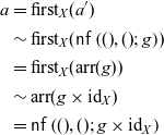 \begin{align*} a & = \mathop{\mathrm{first}}\nolimits_X (a') \\ & \sim \mathop{\mathrm{first}}\nolimits_X(\mathop{\mathsf{nf}}\left({()}, {()}; {g}\right)) \\ & = \mathop{\mathrm{first}}\nolimits_X(\mathop{\mathrm{arr}}\nolimits(g)) \\ & \sim \mathop{\mathrm{arr}}\nolimits(g \times \mathrm{id}_X) \\ & = \mathop{\mathsf{nf}}\left({()}, {()}; {g \times \mathrm{id}_X}\right) \end{align*}
We assume that the claim holds in case n and show the claim in case
 $n + 1$
. We have
$n + 1$
. We have
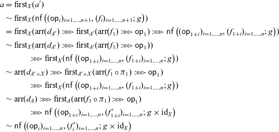 \begin{align*} a & = \mathop{\mathrm{first}}\nolimits_X (a') \\ & \sim \mathop{\mathrm{first}}\nolimits_X(\mathop{\mathsf{nf}}\left({(\mathsf{op}_i)_{i=1,\dots,n+1}}, {(f_i)_{i=1,\dots,n+1}}; {g}\right)) \\ & = \mathop{\mathrm{first}}\nolimits_X(\mathop{\mathrm{arr}}\nolimits(d_{A'}) \mathrel{>\!\!>\!\!>} \mathop{\mathrm{first}}\nolimits_{A'}(\mathop{\mathrm{arr}}\nolimits(f_1) \mathrel{>\!\!>\!\!>} \mathsf{op}_1) \mathrel{>\!\!>\!\!>} \mathop{\mathsf{nf}}\left({(\mathsf{op}_{1 + i})_{i=1,\dots,n}}, {(f_{1 + i})_{i = 1,\dots, n}}; {g}\right)) \\ & \sim \mathop{\mathrm{first}}\nolimits_X(\mathop{\mathrm{arr}}\nolimits(d_{A'}) \mathrel{>\!\!>\!\!>} \mathop{\mathrm{first}}\nolimits_{A'}(\mathop{\mathrm{arr}}\nolimits(f_1) \mathrel{>\!\!>\!\!>} \mathsf{op}_1)) \\ & \hspace{1cm} \mathrel{>\!\!>\!\!>} \mathop{\mathrm{first}}\nolimits_X(\mathop{\mathsf{nf}}\left({(\mathsf{op}_{1 + i})_{i=1,\dots,n}}, {(f_{1 + i})_{i = 1,\dots, n}}; {g}\right)) \\ & \sim \mathop{\mathrm{arr}}\nolimits(d_{A' \times X}) \mathrel{>\!\!>\!\!>} \mathop{\mathrm{first}}\nolimits_{A' \times X} (\mathop{\mathrm{arr}}\nolimits(f_1 \circ \pi_1) \mathrel{>\!\!>\!\!>} \mathsf{op}_1) \\ & \hspace{1cm} \mathrel{>\!\!>\!\!>} \mathop{\mathrm{first}}\nolimits_X(\mathop{\mathsf{nf}}\left({(\mathsf{op}_{1 + i})_{i=1,\dots,n}}, {(f_{1 + i})_{i = 1,\dots, n}}; {g}\right)) \\ & \sim \mathop{\mathrm{arr}}\nolimits(d_{A}) \mathrel{>\!\!>\!\!>} \mathop{\mathrm{first}}\nolimits_{A} (\mathop{\mathrm{arr}}\nolimits(f_1 \circ \pi_1) \mathrel{>\!\!>\!\!>} \mathsf{op}_1) \\ & \hspace{1cm} \mathrel{>\!\!>\!\!>} \mathop{\mathsf{nf}}\left({(\mathsf{op}_{1 + i})_{i=1,\dots,n}}, {(f'_{1 + i})_{i = 1,\dots, n}}; {g \times \mathrm{id}_X}\right) \\ & \sim \mathop{\mathsf{nf}}\left({(\mathsf{op}_{i})_{i=1,\dots,n}}, {(f'_{i})_{i = 1,\dots, n}}; {g \times \mathrm{id}_X}\right) \end{align*}
where
 $f'_1 = f_1 \circ \pi_1 \colon A' \times X \to \mathord{\left[\![{\gamma_1}\right]\!]}$
. See Figure D1.
$f'_1 = f_1 \circ \pi_1 \colon A' \times X \to \mathord{\left[\![{\gamma_1}\right]\!]}$
. See Figure D1.
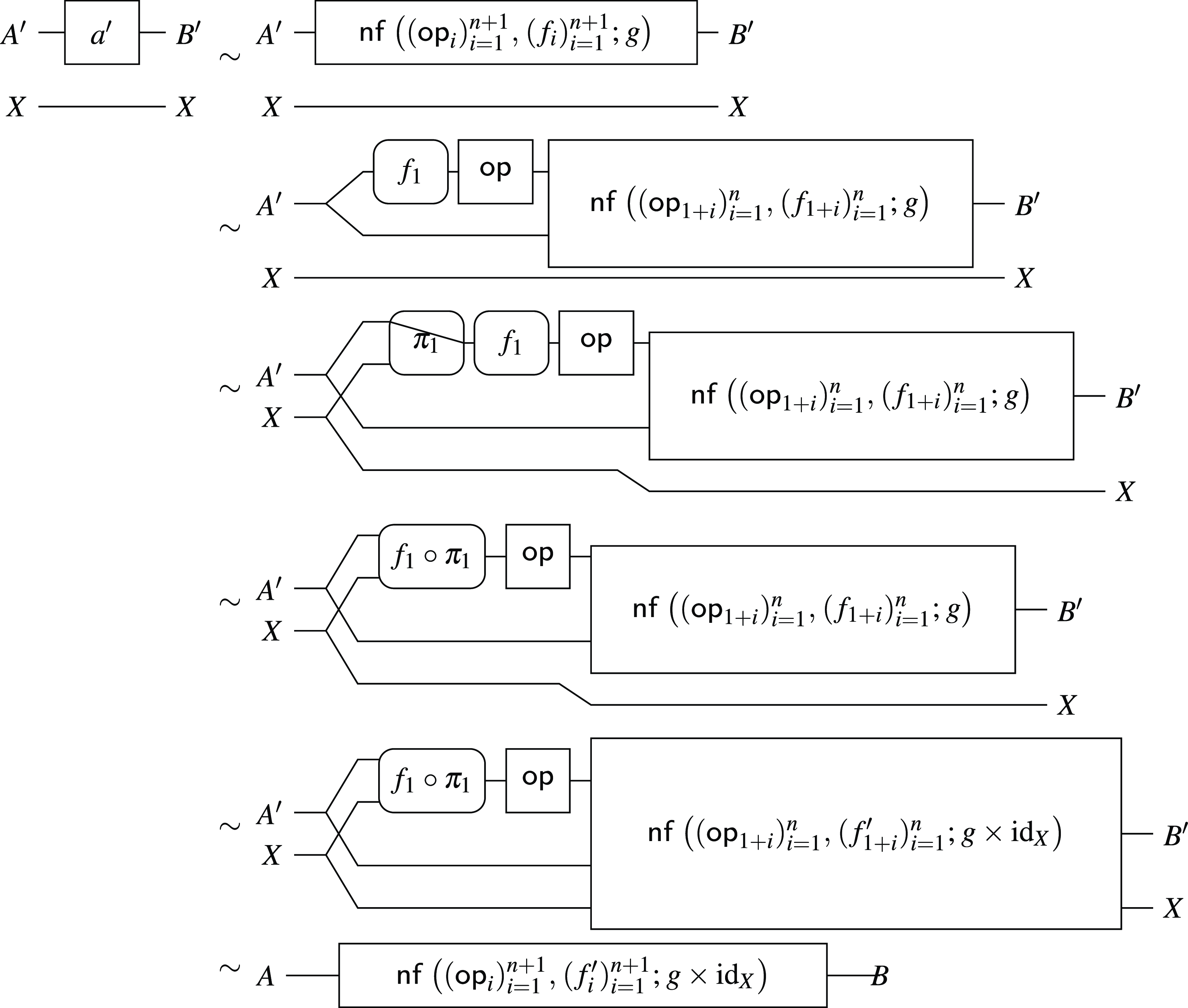
Fig. D1. In case
 $a = \mathop{\mathrm{first}}\nolimits_X(a')$
and
$a = \mathop{\mathrm{first}}\nolimits_X(a')$
and
 $a' \sim \mathop{\mathsf{nf}}\left({(\mathsf{op})_{i=1}^{n+1}}, {(f_i)_{i=1}^{n+1}}; {g}\right)$
.
$a' \sim \mathop{\mathsf{nf}}\left({(\mathsf{op})_{i=1}^{n+1}}, {(f_i)_{i=1}^{n+1}}; {g}\right)$
.
In case
 $a = b \mathrel{>\!\!>\!\!>} c$
for some
$a = b \mathrel{>\!\!>\!\!>} c$
for some
 $b \in \mathrm{Arr}_{\Sigma}(A, X)$
and
$b \in \mathrm{Arr}_{\Sigma}(A, X)$
and
 $c \in \mathrm{Arr}_{\Sigma}(X, B)$
. By the induction hypothesis, we have
$c \in \mathrm{Arr}_{\Sigma}(X, B)$
. By the induction hypothesis, we have
 \begin{equation*} b \sim \mathop{\mathsf{nf}}\left({(\mathsf{op}_i)_{i = 1, \dots, m}}, {(f_i)_{i = 1, \dots, m}}; {g'}\right) \end{equation*}
for some
 $m \in \mathbb{N}$
,
$m \in \mathbb{N}$
, ![]() ,
,
 $(f_i \colon \mathord{\left[\![{\delta_{i-1}}\right]\!]} \times \cdots \times \mathord{\left[\![{\delta_{1}}\right]\!]} \times A \to \mathord{\left[\![{\gamma_i}\right]\!]})_{i = 1 , \dots, m}$
and
$(f_i \colon \mathord{\left[\![{\delta_{i-1}}\right]\!]} \times \cdots \times \mathord{\left[\![{\delta_{1}}\right]\!]} \times A \to \mathord{\left[\![{\gamma_i}\right]\!]})_{i = 1 , \dots, m}$
and
 $g' \colon \mathord{\left[\![{\delta_n}\right]\!]} \times \cdots \times \mathord{\left[\![{\delta_1}\right]\!]} \times A \to X$
, and
$g' \colon \mathord{\left[\![{\delta_n}\right]\!]} \times \cdots \times \mathord{\left[\![{\delta_1}\right]\!]} \times A \to X$
, and
 \begin{equation*} c \sim \mathop{\mathsf{nf}}\left({(\mathsf{op}_{m + i})_{i = 1, \dots, m}}, {(f'_i)_{i = 1, \dots, m}}; {g''}\right) \end{equation*}
for some
 $n \in \mathbb{N}$
,
$n \in \mathbb{N}$
, ![]() ,
,
 $(f'_i \colon \mathord{\left[\![{\delta_{m + i-1}}\right]\!]} \times \cdots \times \mathord{\left[\![{\delta_{m + 1}}\right]\!]} \times A \to \mathord{\left[\![{\gamma_{m + i}}\right]\!]})_{i = 1 , \dots, n}$
and
$(f'_i \colon \mathord{\left[\![{\delta_{m + i-1}}\right]\!]} \times \cdots \times \mathord{\left[\![{\delta_{m + 1}}\right]\!]} \times A \to \mathord{\left[\![{\gamma_{m + i}}\right]\!]})_{i = 1 , \dots, n}$
and
 $g'' \colon \mathord{\left[\![{\delta_{m + n + 1}}\right]\!]} \times \cdots \times \mathord{\left[\![{\delta_{m + 1}}\right]\!]} \times X \to B$
. We show
$g'' \colon \mathord{\left[\![{\delta_{m + n + 1}}\right]\!]} \times \cdots \times \mathord{\left[\![{\delta_{m + 1}}\right]\!]} \times X \to B$
. We show
 $a = b \mathrel{>\!\!>\!\!>} c \sim \mathop{\mathsf{nf}}\left({(\mathsf{op})_{i = 1, \dots, m + n}}, {(f_i)_{i = 1, \dots, m + n}}; {g}\right)$
for some
$a = b \mathrel{>\!\!>\!\!>} c \sim \mathop{\mathsf{nf}}\left({(\mathsf{op})_{i = 1, \dots, m + n}}, {(f_i)_{i = 1, \dots, m + n}}; {g}\right)$
for some
 $(f_i)_{i = m + 1, \dots, m + n}$
and g by induction on n.
$(f_i)_{i = m + 1, \dots, m + n}$
and g by induction on n.
In the base case,
 $n = 0$
, we have
$n = 0$
, we have
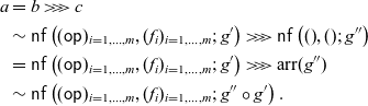 \begin{align*} a & = b \mathrel{>\!\!>\!\!>} c \\ & \sim \mathop{\mathsf{nf}}\left({(\mathsf{op})_{i = 1, \dots, m}}, {(f_i)_{i = 1, \dots, m}}; {g'}\right) \mathrel{>\!\!>\!\!>} \mathop{\mathsf{nf}}\left({()}, {()}; {g''}\right) \\ & = \mathop{\mathsf{nf}}\left({(\mathsf{op})_{i = 1, \dots, m}}, {(f_i)_{i = 1, \dots, m}}; {g'}\right) \mathrel{>\!\!>\!\!>} \mathop{\mathrm{arr}}\nolimits(g'') \\ & \sim \mathop{\mathsf{nf}}\left({(\mathsf{op})_{i = 1, \dots, m}}, {(f_i)_{i = 1, \dots, m}}; {g'' \circ g'}\right). \end{align*}
We assume that the claim holds in case n, and show the claim in case
 $n + 1$
. We have
$n + 1$
. We have
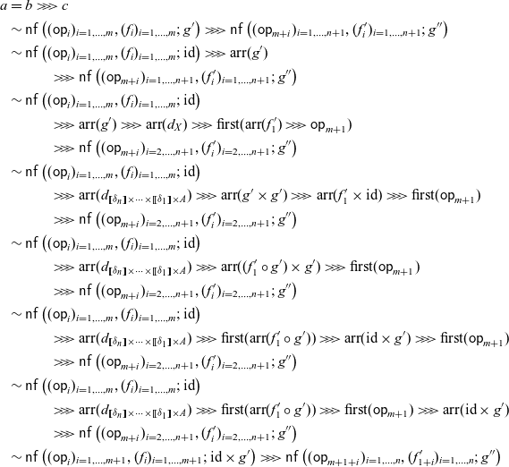 \begin{align*} a & = b \mathrel{>\!\!>\!\!>} c \\ & \sim \mathop{\mathsf{nf}}\left({(\mathsf{op}_i)_{i=1,\dots, m}}, {(f_i)_{i = 1, \dots, m}}; {g'}\right) \mathrel{>\!\!>\!\!>} \mathop{\mathsf{nf}}\left({(\mathsf{op}_{m + i})_{i=1,\dots, n + 1}}, {(f'_i)_{i = 1, \dots, n + 1}}; {g''}\right) \\ & \sim \mathop{\mathsf{nf}}\left({(\mathsf{op}_i)_{i=1,\dots, m}}, {(f_i)_{i = 1, \dots, m}}; {\mathrm{id}}\right) \mathrel{>\!\!>\!\!>} \mathop{\mathrm{arr}}\nolimits(g') \\ & \hspace{1cm} \mathrel{>\!\!>\!\!>} \mathop{\mathsf{nf}}\left({(\mathsf{op}_{m + i})_{i=1,\dots, n + 1}}, {(f'_i)_{i = 1, \dots, n + 1}}; {g''}\right) \\ & \sim \mathop{\mathsf{nf}}\left({(\mathsf{op}_i)_{i=1,\dots, m}}, {(f_i)_{i = 1, \dots, m}}; {\mathrm{id}}\right) \\ & \hspace{1cm} \mathrel{>\!\!>\!\!>} \mathop{\mathrm{arr}}\nolimits(g') \mathrel{>\!\!>\!\!>} \mathop{\mathrm{arr}}\nolimits(d_X) \mathrel{>\!\!>\!\!>} \mathop{\mathrm{first}}\nolimits(\mathop{\mathrm{arr}}\nolimits(f'_1) \mathrel{>\!\!>\!\!>} \mathsf{op}_{m + 1}) \\ & \hspace{1cm} \mathrel{>\!\!>\!\!>} \mathop{\mathsf{nf}}\left({(\mathsf{op}_{m + i})_{i=2,\dots, n + 1}}, {(f'_i)_{i = 2, \dots, n + 1}}; {g''}\right) \\ & \sim \mathop{\mathsf{nf}}\left({(\mathsf{op}_i)_{i=1,\dots, m}}, {(f_i)_{i = 1, \dots, m}}; {\mathrm{id}}\right) \\ & \hspace{1cm} \mathrel{>\!\!>\!\!>} \mathop{\mathrm{arr}}\nolimits(d_{\mathord{\left[\![{\delta_n}\right]\!]} \times \dots \times \mathord{\left[\![{\delta_1}\right]\!]} \times A}) \mathrel{>\!\!>\!\!>} \mathop{\mathrm{arr}}\nolimits(g' \times g') \mathrel{>\!\!>\!\!>} \mathop{\mathrm{arr}}\nolimits(f'_1 \times \mathrm{id}) \mathrel{>\!\!>\!\!>} \mathop{\mathrm{first}}\nolimits(\mathsf{op}_{m + 1}) \\ & \hspace{1cm} \mathrel{>\!\!>\!\!>} \mathop{\mathsf{nf}}\left({(\mathsf{op}_{m + i})_{i=2,\dots, n + 1}}, {(f'_i)_{i = 2, \dots, n + 1}}; {g''}\right) \\ & \sim \mathop{\mathsf{nf}}\left({(\mathsf{op}_i)_{i=1,\dots, m}}, {(f_i)_{i = 1, \dots, m}}; {\mathrm{id}}\right) \\ & \hspace{1cm} \mathrel{>\!\!>\!\!>} \mathop{\mathrm{arr}}\nolimits(d_{\mathord{\left[\![{\delta_n}\right]\!]} \times \dots \times \mathord{\left[\![{\delta_1}\right]\!]} \times A}) \mathrel{>\!\!>\!\!>} \mathop{\mathrm{arr}}\nolimits((f'_1 \circ g') \times g') \mathrel{>\!\!>\!\!>} \mathop{\mathrm{first}}\nolimits(\mathsf{op}_{m + 1}) \\ & \hspace{1cm} \mathrel{>\!\!>\!\!>} \mathop{\mathsf{nf}}\left({(\mathsf{op}_{m + i})_{i=2,\dots, n + 1}}, {(f'_i)_{i = 2, \dots, n + 1}}; {g''}\right) \\ & \sim \mathop{\mathsf{nf}}\left({(\mathsf{op}_i)_{i=1,\dots, m}}, {(f_i)_{i = 1, \dots, m}}; {\mathrm{id}}\right) \\ & \hspace{1cm} \mathrel{>\!\!>\!\!>} \mathop{\mathrm{arr}}\nolimits(d_{\mathord{\left[\![{\delta_n}\right]\!]} \times \dots \times \mathord{\left[\![{\delta_1}\right]\!]} \times A}) \mathrel{>\!\!>\!\!>} \mathop{\mathrm{first}}\nolimits(\mathop{\mathrm{arr}}\nolimits(f'_1 \circ g')) \mathrel{>\!\!>\!\!>} \mathop{\mathrm{arr}}\nolimits(\mathrm{id} \times g') \mathrel{>\!\!>\!\!>} \mathop{\mathrm{first}}\nolimits(\mathsf{op}_{m + 1}) \\ & \hspace{1cm} \mathrel{>\!\!>\!\!>} \mathop{\mathsf{nf}}\left({(\mathsf{op}_{m + i})_{i=2,\dots, n + 1}}, {(f'_i)_{i = 2, \dots, n + 1}}; {g''}\right) \\ & \sim \mathop{\mathsf{nf}}\left({(\mathsf{op}_i)_{i=1,\dots, m}}, {(f_i)_{i = 1, \dots, m}}; {\mathrm{id}}\right) \\ & \hspace{1cm} \mathrel{>\!\!>\!\!>} \mathop{\mathrm{arr}}\nolimits(d_{\mathord{\left[\![{\delta_n}\right]\!]} \times \dots \times \mathord{\left[\![{\delta_1}\right]\!]} \times A}) \mathrel{>\!\!>\!\!>} \mathop{\mathrm{first}}\nolimits(\mathop{\mathrm{arr}}\nolimits(f'_1 \circ g')) \mathrel{>\!\!>\!\!>} \mathop{\mathrm{first}}\nolimits(\mathsf{op}_{m + 1}) \mathrel{>\!\!>\!\!>} \mathop{\mathrm{arr}}\nolimits(\mathrm{id} \times g') \\ & \hspace{1cm} \mathrel{>\!\!>\!\!>} \mathop{\mathsf{nf}}\left({(\mathsf{op}_{m + i})_{i=2,\dots, n + 1}}, {(f'_i)_{i = 2, \dots, n + 1}}; {g''}\right) \\ & \sim \mathop{\mathsf{nf}}\left({(\mathsf{op}_i)_{i=1,\dots, m + 1}}, {(f_i)_{i = 1, \dots, m + 1}}; {\mathrm{id} \times g'}\right) \mathrel{>\!\!>\!\!>} \mathop{\mathsf{nf}}\left({(\mathsf{op}_{m + 1 + i})_{i=1,\dots, n}}, {(f'_{1 + i})_{i = 1, \dots, n}}; {g''}\right) \\ \end{align*}
where
 $f_{m + 1} = f'_1 \circ g'$
. See Figure D2. By the induction hypothesis, we obtain
$f_{m + 1} = f'_1 \circ g'$
. See Figure D2. By the induction hypothesis, we obtain
 \begin{equation*} a \sim \mathop{\mathsf{nf}}\left({(\mathsf{op}_i)_{i = 1, \dots, m + 1 + n}}, {(f_i)_{i = 1, \dots, m + 1 + n}}; {g}\right) \end{equation*}
for some
 $(f_{m + 1 + i})_{i = 1, \dots, n}$
and g.
$(f_{m + 1 + i})_{i = 1, \dots, n}$
and g.
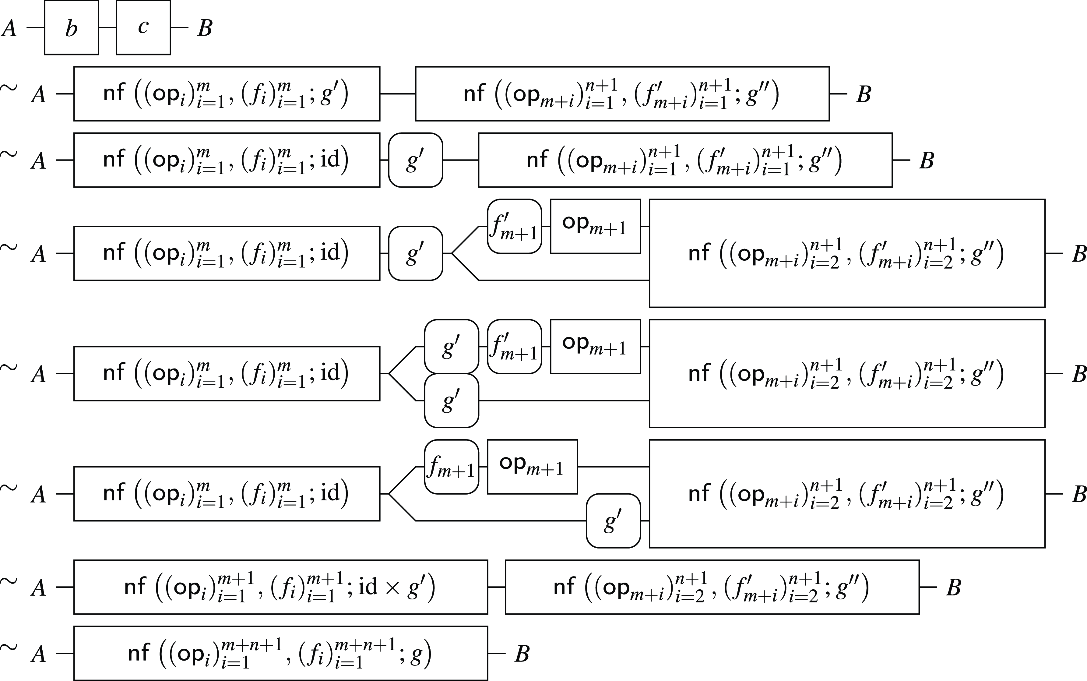
Fig. D2. In case
 $a = b \mathrel{>\!\!>\!\!>} c$
and
$a = b \mathrel{>\!\!>\!\!>} c$
and
 $c \sim \mathop{\mathsf{nf}}\left({(\mathsf{op}_i)_{i=1}^{n + 1}}, {(f'_i)_{i = 1}^{n + 1}}; {g''}\right)$
.
$c \sim \mathop{\mathsf{nf}}\left({(\mathsf{op}_i)_{i=1}^{n + 1}}, {(f'_i)_{i = 1}^{n + 1}}; {g''}\right)$
.
Lemma 5.11. The following hold.
-
1. If
$\Gamma, x : A \vdash M : B$
and
$\Gamma \vdash V : A$
, then
$\mathord{\left[\![{M[V / x]}\right]\!]}^S(c) = \mathord{\left[\![{M}\right]\!]}^S(c, \mathord{\left[\![{V}\right]\!]}^S(c))$
. -
2. If
and
$\Gamma \vdash V : A$
, then
$\mathord{\left[\![{P[V / x]}\right]\!]}^S(c) = \mathord{\left[\![{P}\right]\!]}^S(c, \mathord{\left[\![{V}\right]\!]}^S(c))$
. -
3. If
and
$\Gamma, \Delta \vdash V : A$
, then


Proof. The proof is by induction on the derivations.
(1). In case ![]() . The derivation is
. The derivation is
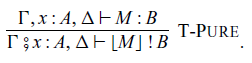
By the induction hypothesis (1), we have
 \begin{equation*} \mathord{\left[\![{M[V / x]}\right]\!]}^S(c, {-}) = \mathord{\left[\![{M}\right]\!]}^S(c, \mathord{\left[\![{V}\right]\!]}^S(c, {-}), {-}) \circ d_{\mathord{\left[\![{\Delta}\right]\!]}^S} \end{equation*}
for any
 $c \in \mathord{\left[\![{\Gamma}\right]\!]}^S$
. Hence, we have
$c \in \mathord{\left[\![{\Gamma}\right]\!]}^S$
. Hence, we have
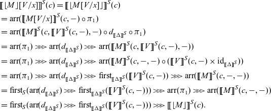 \begin{align*} & \mathord{\left[\![{\lfloor{M}\rfloor[V/x]}\right]\!]}^S(c) = \mathord{\left[\![{\lfloor{M[V/x]}\rfloor}\right]\!]}^S(c) \\ & = \mathop{\mathrm{arr}}\nolimits( \mathord{\left[\![{M[V/x]}\right]\!]}^S(c, {-}) \circ \pi_1 ) \\ & = \mathop{\mathrm{arr}}\nolimits( \mathord{\left[\![{M}\right]\!]}^S(c, \mathord{\left[\![{V}\right]\!]}^S(c, {-}), {-}) \circ d_{\mathord{\left[\![{\Delta}\right]\!]}^S} \circ \pi_1 ) \\ & = \mathop{\mathrm{arr}}\nolimits( \pi_1 ) \mathrel{>\!\!>\!\!>} \mathop{\mathrm{arr}}\nolimits( d_{\mathord{\left[\![{\Delta}\right]\!]}^S} ) \mathrel{>\!\!>\!\!>} \mathop{\mathrm{arr}}\nolimits( \mathord{\left[\![{M}\right]\!]}^S(c, \mathord{\left[\![{V}\right]\!]}^S(c, {-}), {-}) ) \\ & = \mathop{\mathrm{arr}}\nolimits( \pi_1 ) \mathrel{>\!\!>\!\!>} \mathop{\mathrm{arr}}\nolimits( d_{\mathord{\left[\![{\Delta}\right]\!]}^S} ) \mathrel{>\!\!>\!\!>} \mathop{\mathrm{arr}}\nolimits( \mathord{\left[\![{M}\right]\!]}^S(c, {-}, {-}) \circ (\mathord{\left[\![{V}\right]\!]}^S(c, {-}) \times \mathrm{id}_{\mathord{\left[\![{\Delta}\right]\!]}^S})) \\ & = \mathop{\mathrm{arr}}\nolimits( \pi_1 ) \mathrel{>\!\!>\!\!>} \mathop{\mathrm{arr}}\nolimits( d_{\mathord{\left[\![{\Delta}\right]\!]}^S} ) \mathrel{>\!\!>\!\!>} \mathop{\mathrm{first}}\nolimits_{\mathord{\left[\![{\Delta}\right]\!]}^S} ( \mathord{\left[\![{V}\right]\!]}^S(c, {-}) ) \mathrel{>\!\!>\!\!>} \mathop{\mathrm{arr}}\nolimits( \mathord{\left[\![{M}\right]\!]}^S(c, {-}, {-}) ) \\ & = \mathop{\mathrm{first}}\nolimits_S( \mathop{\mathrm{arr}}\nolimits( d_{\mathord{\left[\![{\Delta}\right]\!]}^S} ) \mathrel{>\!\!>\!\!>} \mathop{\mathrm{first}}\nolimits_{\mathord{\left[\![{\Delta}\right]\!]}^S} ( \mathord{\left[\![{V}\right]\!]}^S(c, {-}) ) ) \mathrel{>\!\!>\!\!>} \mathop{\mathrm{arr}}\nolimits(\pi_1) \mathrel{>\!\!>\!\!>} \mathop{\mathrm{arr}}\nolimits( \mathord{\left[\![{M}\right]\!]}^S(c, {-}, {-}) ) \\ & = \mathop{\mathrm{first}}\nolimits_S( \mathop{\mathrm{arr}}\nolimits( d_{\mathord{\left[\![{\Delta}\right]\!]}^S} ) \mathrel{>\!\!>\!\!>} \mathop{\mathrm{first}}\nolimits_{\mathord{\left[\![{\Delta}\right]\!]}^S} ( \mathord{\left[\![{V}\right]\!]}^S(c, {-}) ) ) \mathrel{>\!\!>\!\!>} \mathord{\left[\![{\lfloor{M}\rfloor}\right]\!]}^S(c). \end{align*}
In case ![]() . The derivation is
. The derivation is
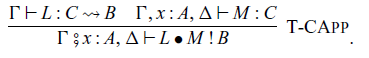
By the induction hypothesis (1), we have
 \begin{equation*} \mathord{\left[\![{M[V / x]}\right]\!]}^S(c, {-}) = \mathord{\left[\![{M}\right]\!]}^S(c, \mathord{\left[\![{V}\right]\!]}^S(c, {-}), {-}) \circ d_{\mathord{\left[\![{\Delta}\right]\!]}^S} \end{equation*}
for any
 $c \in \mathord{\left[\![{\Gamma}\right]\!]}^S$
. Hence, we have
$c \in \mathord{\left[\![{\Gamma}\right]\!]}^S$
. Hence, we have
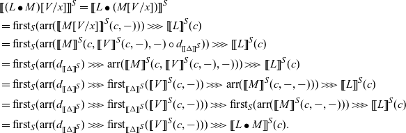 \begin{align*} & \mathord{\left[\![{(L \bullet M)[V / x]}\right]\!]}^S = \mathord{\left[\![{L \bullet (M[V / x])}\right]\!]}^S \\ & = \mathop{\mathrm{first}}\nolimits_S( \mathop{\mathrm{arr}}\nolimits( \mathord{\left[\![{M[V / x]}\right]\!]}^S(c, {-}) ) ) \mathrel{>\!\!>\!\!>} \mathord{\left[\![{L}\right]\!]}^S(c) \\ & = \mathop{\mathrm{first}}\nolimits_S( \mathop{\mathrm{arr}}\nolimits( \mathord{\left[\![{M}\right]\!]}^S(c, \mathord{\left[\![{V}\right]\!]}^S(c, {-}), {-}) \circ d_{\mathord{\left[\![{\Delta}\right]\!]}^S} ) ) \mathrel{>\!\!>\!\!>} \mathord{\left[\![{L}\right]\!]}^S(c) \\ & = \mathop{\mathrm{first}}\nolimits_S( \mathop{\mathrm{arr}}\nolimits(d_{\mathord{\left[\![{\Delta}\right]\!]}^S} ) \mathrel{>\!\!>\!\!>} \mathop{\mathrm{arr}}\nolimits( \mathord{\left[\![{M}\right]\!]}^S(c, \mathord{\left[\![{V}\right]\!]}^S(c, {-}), {-}) ) ) \mathrel{>\!\!>\!\!>} \mathord{\left[\![{L}\right]\!]}^S(c) \\ & = \mathop{\mathrm{first}}\nolimits_S( \mathop{\mathrm{arr}}\nolimits(d_{\mathord{\left[\![{\Delta}\right]\!]}^S} ) \mathrel{>\!\!>\!\!>} \mathop{\mathrm{first}}\nolimits_{\mathord{\left[\![{\Delta}\right]\!]}^S}( \mathord{\left[\![{V}\right]\!]}^S(c, {-}) ) \mathrel{>\!\!>\!\!>} \mathop{\mathrm{arr}}\nolimits( \mathord{\left[\![{M}\right]\!]}^S(c, {-}, {-}) ) ) \mathrel{>\!\!>\!\!>} \mathord{\left[\![{L}\right]\!]}^S(c) \\ & = \mathop{\mathrm{first}}\nolimits_S( \mathop{\mathrm{arr}}\nolimits(d_{\mathord{\left[\![{\Delta}\right]\!]}^S} ) \mathrel{>\!\!>\!\!>} \mathop{\mathrm{first}}\nolimits_{\mathord{\left[\![{\Delta}\right]\!]}^S}( \mathord{\left[\![{V}\right]\!]}^S(c, {-}) ) ) \mathrel{>\!\!>\!\!>} \mathop{\mathrm{first}}\nolimits_S( \mathop{\mathrm{arr}}\nolimits( \mathord{\left[\![{M}\right]\!]}^S(c, {-}, {-}) ) ) \mathrel{>\!\!>\!\!>} \mathord{\left[\![{L}\right]\!]}^S(c) \\ & = \mathop{\mathrm{first}}\nolimits_S( \mathop{\mathrm{arr}}\nolimits(d_{\mathord{\left[\![{\Delta}\right]\!]}^S} ) \mathrel{>\!\!>\!\!>} \mathop{\mathrm{first}}\nolimits_{\mathord{\left[\![{\Delta}\right]\!]}^S}( \mathord{\left[\![{V}\right]\!]}^S(c, {-}) ) ) \mathrel{>\!\!>\!\!>} \mathord{\left[\![{L \bullet M}\right]\!]}^S(c). \end{align*}
In case ![]() . The derivation is
. The derivation is
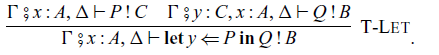
By the induction hypothesis (3), we have
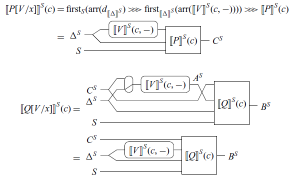
Hence, we have
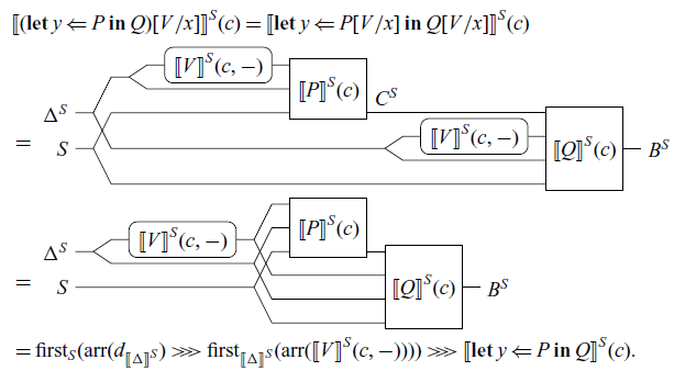
In case ![]() . The derivation is
. The derivation is
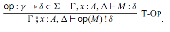
By the induction hypothesis (1), we have
 \begin{equation*} \mathord{\left[\![{M[V / x]}\right]\!]}^S(c, {-}) = \mathord{\left[\![{M}\right]\!]}^S(c, \mathord{\left[\![{V}\right]\!]}^S(c, {-}), {-}) \circ d_{\mathord{\left[\![{\Delta}\right]\!]}^S} \end{equation*}
for any
 $c \in \mathord{\left[\![{\Gamma}\right]\!]}^S$
. Hence, we have
$c \in \mathord{\left[\![{\Gamma}\right]\!]}^S$
. Hence, we have
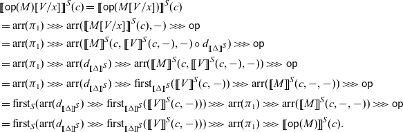 \begin{align*} & \mathord{\left[\![{\mathsf{op}(M)[V / x]}\right]\!]}^S(c) = \mathord{\left[\![{\mathsf{op}(M[V / x])}\right]\!]}^S(c) \\ & = \mathop{\mathrm{arr}}\nolimits(\pi_1) \mathrel{>\!\!>\!\!>} \mathop{\mathrm{arr}}\nolimits( \mathord{\left[\![{M[V/x]}\right]\!]}^S(c), {-} ) \mathrel{>\!\!>\!\!>} \mathsf{op} \\ & = \mathop{\mathrm{arr}}\nolimits(\pi_1) \mathrel{>\!\!>\!\!>} \mathop{\mathrm{arr}}\nolimits( \mathord{\left[\![{M}\right]\!]}^S(c, \mathord{\left[\![{V}\right]\!]}^S(c, {-}), {-}) \circ d_{\mathord{\left[\![{\Delta}\right]\!]}^S} ) \mathrel{>\!\!>\!\!>} \mathsf{op} \\ & = \mathop{\mathrm{arr}}\nolimits(\pi_1) \mathrel{>\!\!>\!\!>} \mathop{\mathrm{arr}}\nolimits( d_{\mathord{\left[\![{\Delta}\right]\!]}^S} ) \mathrel{>\!\!>\!\!>} \mathop{\mathrm{arr}}\nolimits( \mathord{\left[\![{M}\right]\!]}^S(c, \mathord{\left[\![{V}\right]\!]}^S(c, {-}), {-}) ) \mathrel{>\!\!>\!\!>} \mathsf{op} \\ & = \mathop{\mathrm{arr}}\nolimits(\pi_1) \mathrel{>\!\!>\!\!>} \mathop{\mathrm{arr}}\nolimits( d_{\mathord{\left[\![{\Delta}\right]\!]}^S} ) \mathrel{>\!\!>\!\!>} \mathop{\mathrm{first}}\nolimits_{\mathord{\left[\![{\Delta}\right]\!]}^S}(\mathord{\left[\![{V}\right]\!]}^S(c, {-})) \mathrel{>\!\!>\!\!>} \mathop{\mathrm{arr}}\nolimits( \mathord{\left[\![{M}\right]\!]}^S(c, {-}, {-}) ) \mathrel{>\!\!>\!\!>} \mathsf{op} \\ & = \mathop{\mathrm{first}}\nolimits_S(\mathop{\mathrm{arr}}\nolimits( d_{\mathord{\left[\![{\Delta}\right]\!]}^S} ) \mathrel{>\!\!>\!\!>} \mathop{\mathrm{first}}\nolimits_{\mathord{\left[\![{\Delta}\right]\!]}^S}(\mathord{\left[\![{V}\right]\!]}^S(c, {-}))) \mathrel{>\!\!>\!\!>} \mathop{\mathrm{arr}}\nolimits(\pi_1) \mathrel{>\!\!>\!\!>} \mathop{\mathrm{arr}}\nolimits( \mathord{\left[\![{M}\right]\!]}^S(c, {-}, {-}) ) \mathrel{>\!\!>\!\!>} \mathsf{op} \\ & = \mathop{\mathrm{first}}\nolimits_S(\mathop{\mathrm{arr}}\nolimits( d_{\mathord{\left[\![{\Delta}\right]\!]}^S} ) \mathrel{>\!\!>\!\!>} \mathop{\mathrm{first}}\nolimits_{\mathord{\left[\![{\Delta}\right]\!]}^S}(\mathord{\left[\![{V}\right]\!]}^S(c, {-}))) \mathrel{>\!\!>\!\!>} \mathop{\mathrm{arr}}\nolimits(\pi_1) \mathrel{>\!\!>\!\!>} \mathord{\left[\![{\mathsf{op}(M)}\right]\!]}^S(c). \end{align*}
In case ![]() . The derivation is
. The derivation is
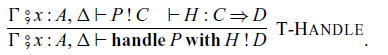
By the induction hypothesis (3), we have
 \begin{equation*} \mathord{\left[\![{P[V / x]}\right]\!]}^S(c) = \mathop{\mathrm{first}}\nolimits_{S}(\mathop{\mathrm{arr}}\nolimits(d_{\mathord{\left[\![{\Delta}\right]\!]}^S}) \mathrel{>\!\!>\!\!>} \mathop{\mathrm{first}}\nolimits_{\mathord{\left[\![{\Delta}\right]\!]}^S}(\mathop{\mathrm{arr}}\nolimits(\mathord{\left[\![{V}\right]\!]}^S(c, {-})))) \mathrel{>\!\!>\!\!>} \mathord{\left[\![{P}\right]\!]}^S(c). \end{equation*}
Hence, we have
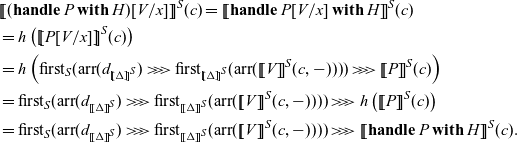 \begin{align*} & \mathord{\left[\![{(\mathop{\mathbf{handle}} P \mathop{\mathbf{with}} H)[V / x]}\right]\!]}^S(c) = \mathord{\left[\![{\mathop{\mathbf{handle}} P[V / x] \mathop{\mathbf{with}} H}\right]\!]}^S(c) \\ & = h\left( \mathord{\left[\![{ P[V / x] }\right]\!]}^S(c) \right) \\ & = h\left( \mathop{\mathrm{first}}\nolimits_{S}(\mathop{\mathrm{arr}}\nolimits(d_{\mathord{\left[\![{\Delta}\right]\!]}^S}) \mathrel{>\!\!>\!\!>} \mathop{\mathrm{first}}\nolimits_{\mathord{\left[\![{\Delta}\right]\!]}^S}(\mathop{\mathrm{arr}}\nolimits(\mathord{\left[\![{V}\right]\!]}^S(c, {-})))) \mathrel{>\!\!>\!\!>} \mathord{\left[\![{P}\right]\!]}^S(c) \right) \\ & = \mathop{\mathrm{first}}\nolimits_{S}(\mathop{\mathrm{arr}}\nolimits(d_{\mathord{\left[\![{\Delta}\right]\!]}^S}) \mathrel{>\!\!>\!\!>} \mathop{\mathrm{first}}\nolimits_{\mathord{\left[\![{\Delta}\right]\!]}^S}(\mathop{\mathrm{arr}}\nolimits(\mathord{\left[\![{V}\right]\!]}^S(c, {-})))) \mathrel{>\!\!>\!\!>} h\left( \mathord{\left[\![{P}\right]\!]}^S(c) \right) \\ & = \mathop{\mathrm{first}}\nolimits_{S}(\mathop{\mathrm{arr}}\nolimits(d_{\mathord{\left[\![{\Delta}\right]\!]}^S}) \mathrel{>\!\!>\!\!>} \mathop{\mathrm{first}}\nolimits_{\mathord{\left[\![{\Delta}\right]\!]}^S}(\mathop{\mathrm{arr}}\nolimits(\mathord{\left[\![{V}\right]\!]}^S(c, {-})))) \mathrel{>\!\!>\!\!>} \mathord{\left[\![{\mathop{\mathbf{handle}} P \mathop{\mathbf{with}} H}\right]\!]}^S(c). \end{align*}
Lemma 5.12. If ![]() , then
, then
 \begin{equation*} \mathord{\left[\![{\mathcal{F}[\mathsf{op}(V)]}\right]\!]}^S(\star) = \mathop{\mathrm{first}}\nolimits_S(\mathop{\mathrm{arr}}\nolimits(\mathord{\left[\![{V}\right]\!]}^S) \mathrel{>\!\!>\!\!>} \mathsf{op}) \mathrel{>\!\!>\!\!>} \mathord{\left[\![{\mathcal{F}[\lfloor{y}\rfloor]}\right]\!]}^S(\star) \end{equation*}
holds.
Proof The proof is by induction on the structure of
 $\mathcal{F}$
.
$\mathcal{F}$
.
If
 $\mathcal{F} = [{-}]$
, then we have
$\mathcal{F} = [{-}]$
, then we have
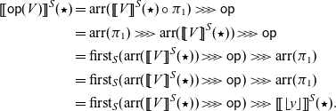 \begin{align*} \mathord{\left[\![{\mathsf{op}(V)}\right]\!]}^S(\star) & = \mathop{\mathrm{arr}}\nolimits(\mathord{\left[\![{V}\right]\!]}^S(\star) \circ \pi_1) \mathrel{>\!\!>\!\!>} \mathsf{op} \\ & = \mathop{\mathrm{arr}}\nolimits(\pi_1) \mathrel{>\!\!>\!\!>} \mathop{\mathrm{arr}}\nolimits(\mathord{\left[\![{V}\right]\!]}^S(\star)) \mathrel{>\!\!>\!\!>} \mathsf{op} \\ & = \mathop{\mathrm{first}}\nolimits_S(\mathop{\mathrm{arr}}\nolimits(\mathord{\left[\![{V}\right]\!]}^S(\star)) \mathrel{>\!\!>\!\!>} \mathsf{op}) \mathrel{>\!\!>\!\!>} \mathop{\mathrm{arr}}\nolimits(\pi_1) \\ & = \mathop{\mathrm{first}}\nolimits_S(\mathop{\mathrm{arr}}\nolimits(\mathord{\left[\![{V}\right]\!]}^S(\star)) \mathrel{>\!\!>\!\!>} \mathsf{op}) \mathrel{>\!\!>\!\!>} \mathop{\mathrm{arr}}\nolimits(\pi_1) \\ & = \mathop{\mathrm{first}}\nolimits_S(\mathop{\mathrm{arr}}\nolimits(\mathord{\left[\![{V}\right]\!]}^S(\star)) \mathrel{>\!\!>\!\!>} \mathsf{op}) \mathrel{>\!\!>\!\!>} \mathord{\left[\![{\lfloor{y}\rfloor}\right]\!]}^S(\star). \end{align*}
Otherwise,
 $\mathcal{F} = (\mathop{\mathbf{let}} x \Leftarrow \mathcal{F}' \mathop{\mathbf{in}} P)$
, we have
$\mathcal{F} = (\mathop{\mathbf{let}} x \Leftarrow \mathcal{F}' \mathop{\mathbf{in}} P)$
, we have
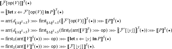 \begin{align*} & \mathord{\left[\![{\mathcal{F}[\mathsf{op}(V)]}\right]\!]}^S(\star) \\ & = \mathord{\left[\![{\mathop{\mathbf{let}} x \Leftarrow \mathcal{F}'[\mathsf{op}(V)] \mathop{\mathbf{in}} P}\right]\!]}^S(\star) \\ & = \mathop{\mathrm{arr}}\nolimits(d_{\mathord{\left[\![{\Delta}\right]\!]}^S \times S}) \mathrel{>\!\!>\!\!>} \mathop{\mathrm{first}}\nolimits_{\mathord{\left[\![{\Delta}\right]\!]}^S \times S}(\mathord{\left[\![{\mathcal{F}'[\mathsf{op}(V)]}\right]\!]}^S(\star)) \mathrel{>\!\!>\!\!>} \mathord{\left[\![{P}\right]\!]}^S(\star) \\ & = \mathop{\mathrm{arr}}\nolimits(d_{\mathord{\left[\![{\Delta}\right]\!]}^S \times S}) \mathrel{>\!\!>\!\!>} \mathop{\mathrm{first}}\nolimits_{\mathord{\left[\![{\Delta}\right]\!]}^S \times S}( \mathop{\mathrm{first}}\nolimits_S(\mathop{\mathrm{arr}}\nolimits(\mathord{\left[\![{V}\right]\!]}^S) \mathrel{>\!\!>\!\!>} \mathsf{op}) \mathrel{>\!\!>\!\!>} \mathord{\left[\![{\mathcal{F}'[\lfloor{y}\rfloor]}\right]\!]}^S(\star) ) \mathrel{>\!\!>\!\!>} \mathord{\left[\![{P}\right]\!]}^S(\star) \\ & = \mathop{\mathrm{first}}\nolimits_S(\mathop{\mathrm{arr}}\nolimits(\mathord{\left[\![{V}\right]\!]}^S(\star)) \mathrel{>\!\!>\!\!>} \mathsf{op}) \mathrel{>\!\!>\!\!>} \mathord{\left[\![{\mathop{\mathbf{let}} x \Leftarrow \lfloor{y}\rfloor \mathop{\mathbf{in}} P}\right]\!]}^S(\star) \\ & = \mathop{\mathrm{first}}\nolimits_S(\mathop{\mathrm{arr}}\nolimits(\mathord{\left[\![{V}\right]\!]}^S(\star)) \mathrel{>\!\!>\!\!>} \mathsf{op}) \mathrel{>\!\!>\!\!>} \mathord{\left[\![{\mathcal{F}[\lfloor{y}\rfloor]}\right]\!]}^S(\star). \end{align*}
by the induction hypothesis.
Theorem 5.13 (soundness). The following hold.
-
1. If
$\diamond \vdash M : A$
and
$M \to M'$
, then
$\mathord{\left[\![{M}\right]\!]}^S = \mathord{\left[\![{M'}\right]\!]}^S$
for any S. -
2. If
and
$P \to P'$
, then
$\mathord{\left[\![{P}\right]\!]}^S = \mathord{\left[\![{P'}\right]\!]}^S$
for any S.


Proof By induction on the derivations
 $M \to M'$
and
$M \to M'$
and
 $P \to P'$
.
$P \to P'$
.
(1). In case ![]() . We have
. We have
 $\diamond \vdash \mathop{\mathbf{fst}} \langle {V_1}, {V_2} \rangle : A_1$
and
$\diamond \vdash \mathop{\mathbf{fst}} \langle {V_1}, {V_2} \rangle : A_1$
and
 $\mathop{\mathbf{fst}} \langle {V_1}, {V_2} \rangle \to V_1$
. The derivation of
$\mathop{\mathbf{fst}} \langle {V_1}, {V_2} \rangle \to V_1$
. The derivation of
 $\diamond \vdash \mathop{\mathbf{fst}} \langle {V_1}, {V_2} \rangle : A_1$
is
$\diamond \vdash \mathop{\mathbf{fst}} \langle {V_1}, {V_2} \rangle : A_1$
is
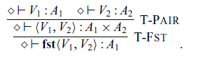
We have
 \begin{equation*} \mathord{\left[\![{\mathop{\mathbf{fst}} \langle {V_1}, {V_2} \rangle}\right]\!]}^S(\star) = \pi_1 (\mathord{\left[\![{V_1}\right]\!]}^S(\star), \mathord{\left[\![{V_2}\right]\!]}^S(\star)) = \mathord{\left[\![{V_1}\right]\!]}^S(\star) \end{equation*}
for any S and
 $\star \in \mathord{\left[\![{\diamond}\right]\!]}^S = 1 = \{ \star \}$
.
$\star \in \mathord{\left[\![{\diamond}\right]\!]}^S = 1 = \{ \star \}$
.
In case ![]() . Similar to the case
. Similar to the case ![]() .
.
In case ![]() . We have
. We have
 $\diamond \vdash (\lambda x : A. M) V : B$
and
$\diamond \vdash (\lambda x : A. M) V : B$
and
 $(\lambda x : A . M) V \to M[V / x]$
. The derivation of
$(\lambda x : A . M) V \to M[V / x]$
. The derivation of
 $\diamond \vdash (\lambda x : A. M) V : B$
is
$\diamond \vdash (\lambda x : A. M) V : B$
is
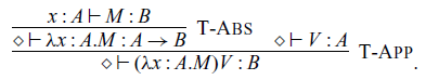
We have
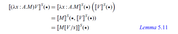
for any S and
 $\star \in \mathord{\left[\![{\diamond}\right]\!]}^S = 1 = \{ \star \}$
.
$\star \in \mathord{\left[\![{\diamond}\right]\!]}^S = 1 = \{ \star \}$
.
In case ![]() . We have
. We have
 $\diamond \vdash \mathcal{E}[M] : A$
and
$\diamond \vdash \mathcal{E}[M] : A$
and
 $\mathcal{E}[M] \to \mathcal{E}[M']$
. From the derivation of
$\mathcal{E}[M] \to \mathcal{E}[M']$
. From the derivation of
 $\mathcal{E}[M] \to \mathcal{E}[M']$
, we have
$\mathcal{E}[M] \to \mathcal{E}[M']$
, we have
 $M \to M'$
. By the induction hypothesis, we have
$M \to M'$
. By the induction hypothesis, we have
 $\mathord{\left[\![{M}\right]\!]}^S = \mathord{\left[\![{M'}\right]\!]}^S$
. We obtain
$\mathord{\left[\![{M}\right]\!]}^S = \mathord{\left[\![{M'}\right]\!]}^S$
. We obtain
 $\mathord{\left[\![{\mathcal{E}[M]}\right]\!]}^S = \mathord{\left[\![{\mathcal{E}[M']}\right]\!]}^S$
by induction on the structure of
$\mathord{\left[\![{\mathcal{E}[M]}\right]\!]}^S = \mathord{\left[\![{\mathcal{E}[M']}\right]\!]}^S$
by induction on the structure of
 $\mathcal{E}$
.
$\mathcal{E}$
.
(2). In case ![]() . We have
. We have ![]() and
and
 $(\lambda^{\bullet} x : A . P) \bullet V \to P[V / x]$
. The derivation of
$(\lambda^{\bullet} x : A . P) \bullet V \to P[V / x]$
. The derivation of ![]() is
is
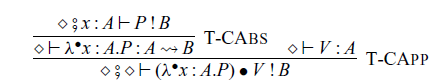
We have
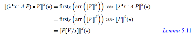
for any S and
 $\star \in \mathord{\left[\![{\Gamma}\right]\!]}^S = 1 = \{ \star \}$
.
$\star \in \mathord{\left[\![{\Gamma}\right]\!]}^S = 1 = \{ \star \}$
.
In case ![]() . We have
. We have ![]() and
and
 $\mathop{\mathbf{let}} x \Leftarrow \lfloor{V}\rfloor \mathop{\mathbf{in}} Q \to Q[V / x]$
. The derivation of
$\mathop{\mathbf{let}} x \Leftarrow \lfloor{V}\rfloor \mathop{\mathbf{in}} Q \to Q[V / x]$
. The derivation of ![]() is
is
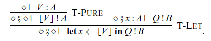
We have
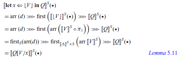
for any S and
 $\star \in \mathord{\left[\![{\diamond}\right]\!]}^S = 1 = \{ \star \}$
.
$\star \in \mathord{\left[\![{\diamond}\right]\!]}^S = 1 = \{ \star \}$
.
In case ![]() . We have
. We have ![]() and
and
 $\mathop{\mathbf{handle}} \lfloor{V}\rfloor \mathop{\mathbf{with}} H \to P[V / x]$
where
$\mathop{\mathbf{handle}} \lfloor{V}\rfloor \mathop{\mathbf{with}} H \to P[V / x]$
where ![]() . The derivation of
. The derivation of ![]() is
is
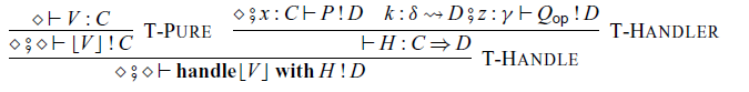
where C and D are primitive. We have
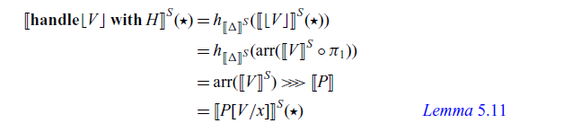
for any S and
 $\star \in \mathord{\left[\![{\diamond}\right]\!]}^S = 1 = \{ \star \}$
.
$\star \in \mathord{\left[\![{\diamond}\right]\!]}^S = 1 = \{ \star \}$
.
In case ![]() . We have
. We have ![]() and
and
 $\mathop{\mathbf{handle}} \mathcal{F}[op(V)] \mathop{\mathbf{with}} H \to Q_{\mathsf{op}}[V / z, (\lambda^{\bullet} y : \delta . \mathop{\mathbf{handle}} \mathcal{F}[\lfloor{y}\rfloor] \mathop{\mathbf{with}} H) / k]$
where
$\mathop{\mathbf{handle}} \mathcal{F}[op(V)] \mathop{\mathbf{with}} H \to Q_{\mathsf{op}}[V / z, (\lambda^{\bullet} y : \delta . \mathop{\mathbf{handle}} \mathcal{F}[\lfloor{y}\rfloor] \mathop{\mathbf{with}} H) / k]$
where ![]() . The derivation of
. The derivation of ![]() is
is
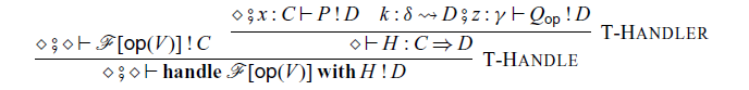
where C and D are primitive. We have
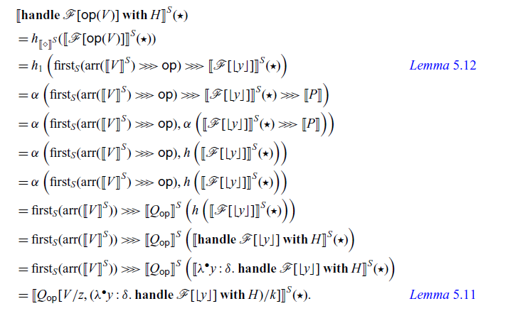
In case ![]() . We have
. We have ![]() and
and
 $\mathcal{F}[P] \to \mathcal{F}[P']$
. From the derivation of
$\mathcal{F}[P] \to \mathcal{F}[P']$
. From the derivation of
 $\mathcal{F}[P] \to \mathcal{F}[P']$
, we have
$\mathcal{F}[P] \to \mathcal{F}[P']$
, we have
 $P \to P'$
. By the induction hypothesis, we have
$P \to P'$
. By the induction hypothesis, we have
 $\mathord{\left[\![{P}\right]\!]}^S = \mathord{\left[\![{P'}\right]\!]}^S$
.
$\mathord{\left[\![{P}\right]\!]}^S = \mathord{\left[\![{P'}\right]\!]}^S$
.
We show
 $\mathord{\left[\![{\mathcal{F}[P]}\right]\!]}^S = \mathord{\left[\![{\mathcal{F}[P']}\right]\!]}^S$
by induction on the structure of
$\mathord{\left[\![{\mathcal{F}[P]}\right]\!]}^S = \mathord{\left[\![{\mathcal{F}[P']}\right]\!]}^S$
by induction on the structure of
 $\mathcal{F}$
. If
$\mathcal{F}$
. If
 $\mathcal{F} = [{-}]$
, we have nothing to do. Suppose
$\mathcal{F} = [{-}]$
, we have nothing to do. Suppose
 $\mathcal{F} = \mathop{\mathbf{let}} x \Leftarrow \mathcal{F}' \mathop{\mathbf{in}} Q$
. By the induction hypothesis, we have
$\mathcal{F} = \mathop{\mathbf{let}} x \Leftarrow \mathcal{F}' \mathop{\mathbf{in}} Q$
. By the induction hypothesis, we have
 $\mathord{\left[\![{\mathcal{F}'[P]}\right]\!]}^S = \mathord{\left[\![{\mathcal{F}'[P']}\right]\!]}^S$
. From the definition of the interpretation of
$\mathord{\left[\![{\mathcal{F}'[P]}\right]\!]}^S = \mathord{\left[\![{\mathcal{F}'[P']}\right]\!]}^S$
. From the definition of the interpretation of
 $\mathop{\mathbf{let}} x \Leftarrow R \mathop{\mathbf{in}} Q$
, we obtain
$\mathop{\mathbf{let}} x \Leftarrow R \mathop{\mathbf{in}} Q$
, we obtain
 $\mathord{\left[\![{\mathcal{F}[P]}\right]\!]}^S = \mathord{\left[\![{\mathop{\mathbf{let}} x \Leftarrow \mathcal{F}'[P] \mathop{\mathbf{in}} Q}\right]\!]}^S = \mathord{\left[\![{\mathop{\mathbf{let}} x \Leftarrow \mathcal{F}'[P'] \mathop{\mathbf{in}} Q}\right]\!]}^S = \mathord{\left[\![{\mathcal{F}[P']}\right]\!]}^S$
.
$\mathord{\left[\![{\mathcal{F}[P]}\right]\!]}^S = \mathord{\left[\![{\mathop{\mathbf{let}} x \Leftarrow \mathcal{F}'[P] \mathop{\mathbf{in}} Q}\right]\!]}^S = \mathord{\left[\![{\mathop{\mathbf{let}} x \Leftarrow \mathcal{F}'[P'] \mathop{\mathbf{in}} Q}\right]\!]}^S = \mathord{\left[\![{\mathcal{F}[P']}\right]\!]}^S$
.
Lemma 5.15. The following hold.
-
1. If
$M \to^* M'$
and
$v \triangleleft_A M'$
, then
$v \triangleleft_A M$
. -
2. If
$M \to^* M'$
and
$v \triangleleft_A M$
, then
$v \triangleleft_A M'$
. -
3. If
$P \to^* P'$
and
$a \blacktriangleleft_A P'$
, then
$a \blacktriangleleft_A P$
. -
4. If
$P \to^* P'$
and
$a \blacktriangleleft_A P$
, then
$a \blacktriangleleft_A P'$
.


Proof We can prove (3) and (4) straightforwardly by the definition. To prove (1) and (2), we do induction on the type A.
(1). In case Unit. Suppose
 $M \to^* M'$
and
$M \to^* M'$
and
 $v \triangleleft_{\mathrm{Unit}} M'$
. We have
$v \triangleleft_{\mathrm{Unit}} M'$
. We have
 $v = \star$
and
$v = \star$
and
 $M' \to^* \mathtt{\langle\rangle}$
by the definition of
$M' \to^* \mathtt{\langle\rangle}$
by the definition of
 $\triangleleft_{\mathrm{Unit}}$
. Hence, we have
$\triangleleft_{\mathrm{Unit}}$
. Hence, we have
 $M \to^* M' \to^* \mathtt{\langle\rangle}$
, which means
$M \to^* M' \to^* \mathtt{\langle\rangle}$
, which means
 $v \triangleleft_{\mathrm{Unit}} M$
.
$v \triangleleft_{\mathrm{Unit}} M$
.
In case
 $A_1 \times A_2$
. Suppose
$A_1 \times A_2$
. Suppose
 $M \to^* M'$
and
$M \to^* M'$
and
 $v \triangleleft_{A_1 \times A_2} M'$
. We have
$v \triangleleft_{A_1 \times A_2} M'$
. We have
 $M \to^* M' \to^* \langle {V_1}, {V_2} \rangle$
,
$M \to^* M' \to^* \langle {V_1}, {V_2} \rangle$
,
 $\pi_1(v) \triangleleft_{A_1} V_1$
and
$\pi_1(v) \triangleleft_{A_1} V_1$
and
 $\pi_2(v) \triangleleft_{A_2} V_2$
. This means
$\pi_2(v) \triangleleft_{A_2} V_2$
. This means
 $v \triangleleft_{A_1 \times A_2} M$
.
$v \triangleleft_{A_1 \times A_2} M$
.
In case
 $A \to B$
. Suppose
$A \to B$
. Suppose
 $M \to^* M'$
and
$M \to^* M'$
and
 $f \triangleleft_{A \to B} M'$
. We have
$f \triangleleft_{A \to B} M'$
. We have
 $M \to^* M' \to^* \lambda x : A . M''$
and
$M \to^* M' \to^* \lambda x : A . M''$
and
 $(w \triangleleft_{A} N \implies fw \triangleleft_{B} M'N)$
for any N and w. Given N and w with
$(w \triangleleft_{A} N \implies fw \triangleleft_{B} M'N)$
for any N and w. Given N and w with
 $w \triangleleft_{A} N$
, we have
$w \triangleleft_{A} N$
, we have
 $fw \triangleleft_{B} M'N$
. Since
$fw \triangleleft_{B} M'N$
. Since
 $M \to^* M'$
, we have
$M \to^* M'$
, we have
 $MN \to^* M'N$
. By the induction hypothesis (1), we have
$MN \to^* M'N$
. By the induction hypothesis (1), we have
 $fw \triangleleft_{B} MN$
. This means
$fw \triangleleft_{B} MN$
. This means
 $f \triangleleft_{A \to B} M$
.
$f \triangleleft_{A \to B} M$
.
In case
 $A \rightsquigarrow B$
. Suppose
$A \rightsquigarrow B$
. Suppose
 $M \to^* M'$
and
$M \to^* M'$
and
 $a \triangleleft_{A \rightsquigarrow B} M'$
. We have
$a \triangleleft_{A \rightsquigarrow B} M'$
. We have
 $M \to^* M' \to^* \lambda^{\bullet} x : A . P$
and
$M \to^* M' \to^* \lambda^{\bullet} x : A . P$
and
 $(w \triangleleft_{A} N \implies \mathop{\mathrm{arr}}\nolimits(w) \mathrel{>\!\!>\!\!>} a \blacktriangleleft_{B} M' \bullet N)$
for any N and w. Given N and w with
$(w \triangleleft_{A} N \implies \mathop{\mathrm{arr}}\nolimits(w) \mathrel{>\!\!>\!\!>} a \blacktriangleleft_{B} M' \bullet N)$
for any N and w. Given N and w with
 $w \triangleleft_{A} N$
, we have
$w \triangleleft_{A} N$
, we have
 $\mathop{\mathrm{arr}}\nolimits(w) \mathrel{>\!\!>\!\!>} a \blacktriangleleft_{B} M' \bullet N$
. Since
$\mathop{\mathrm{arr}}\nolimits(w) \mathrel{>\!\!>\!\!>} a \blacktriangleleft_{B} M' \bullet N$
. Since
 $M \to^* M'$
, we have
$M \to^* M'$
, we have
 $M \bullet N \to^* M' \bullet N$
. By (3), we have
$M \bullet N \to^* M' \bullet N$
. By (3), we have
 $\mathop{\mathrm{arr}}\nolimits(w) \mathrel{>\!\!>\!\!>} a \blacktriangleleft_{B} M \bullet N$
. This means
$\mathop{\mathrm{arr}}\nolimits(w) \mathrel{>\!\!>\!\!>} a \blacktriangleleft_{B} M \bullet N$
. This means
 $a \triangleleft_{A \rightsquigarrow B} M$
.
$a \triangleleft_{A \rightsquigarrow B} M$
.
(2). Note that we can show that
 $M' \to^* V$
if
$M' \to^* V$
if
 $M \to^* V$
and
$M \to^* V$
and
 $M \to^* M'$
.
$M \to^* M'$
.
In case Unit. Suppose
 $M \to^* M'$
and
$M \to^* M'$
and
 $v \triangleleft_{\mathrm{Unit}} M$
. We have
$v \triangleleft_{\mathrm{Unit}} M$
. We have
 $v = \star$
and
$v = \star$
and
 $M \to^* \mathtt{\langle\rangle}$
by the definition of
$M \to^* \mathtt{\langle\rangle}$
by the definition of
 $\triangleleft_{\mathrm{Unit}}$
. Hence, we have
$\triangleleft_{\mathrm{Unit}}$
. Hence, we have
 $M' \to^* \mathtt{\langle\rangle}$
, which means
$M' \to^* \mathtt{\langle\rangle}$
, which means
 $v \triangleleft_{\mathrm{Unit}} M'$
.
$v \triangleleft_{\mathrm{Unit}} M'$
.
In case
 $A_1 \times A_2$
. Suppose
$A_1 \times A_2$
. Suppose
 $M \to^* M'$
and
$M \to^* M'$
and
 $v \triangleleft_{A_1 \times A_2} M$
. We have
$v \triangleleft_{A_1 \times A_2} M$
. We have
 $M \to^* \langle {V_1}, {V_2} \rangle$
,
$M \to^* \langle {V_1}, {V_2} \rangle$
,
 $\pi_1(v) \triangleleft_{A_1} V_1$
and
$\pi_1(v) \triangleleft_{A_1} V_1$
and
 $\pi_2(v) \triangleleft_{A_2} V_2$
. This means
$\pi_2(v) \triangleleft_{A_2} V_2$
. This means
 $v \triangleleft_{A_1 \times A_2} M$
since we have
$v \triangleleft_{A_1 \times A_2} M$
since we have
 $M' \to^* \langle {V_1}, {V_2} \rangle$
.
$M' \to^* \langle {V_1}, {V_2} \rangle$
.
In case
 $A \to B$
. Suppose
$A \to B$
. Suppose
 $M \to^* M'$
and
$M \to^* M'$
and
 $f \triangleleft_{A \to B} M$
. We have
$f \triangleleft_{A \to B} M$
. We have
 $M \to^* \lambda x : A . M''$
and
$M \to^* \lambda x : A . M''$
and
 $(w \triangleleft_{A} N \implies fw \triangleleft_{B} MN)$
for any N and w. Given N and w with
$(w \triangleleft_{A} N \implies fw \triangleleft_{B} MN)$
for any N and w. Given N and w with
 $w \triangleleft_{A} N$
, we have
$w \triangleleft_{A} N$
, we have
 $fw \triangleleft_{B} MN$
. Since
$fw \triangleleft_{B} MN$
. Since
 $M \to^* M'$
, we have
$M \to^* M'$
, we have
 $MN \to^* M'N$
. By the induction hypothesis (2), we have
$MN \to^* M'N$
. By the induction hypothesis (2), we have
 $fw \triangleleft_{B} M'N$
. This means
$fw \triangleleft_{B} M'N$
. This means
 $f \triangleleft_{A \to B} M'$
.
$f \triangleleft_{A \to B} M'$
.
In case
 $A \rightsquigarrow B$
. Suppose
$A \rightsquigarrow B$
. Suppose
 $M \to^* M'$
and
$M \to^* M'$
and
 $a \triangleleft_{A \rightsquigarrow B} M$
. We have
$a \triangleleft_{A \rightsquigarrow B} M$
. We have
 $M \to^* \lambda^{\bullet} x : A . P$
and
$M \to^* \lambda^{\bullet} x : A . P$
and
 $(w \triangleleft_{A} N \implies \mathop{\mathrm{arr}}\nolimits(w) \mathrel{>\!\!>\!\!>} a \blacktriangleleft_{B} M \bullet N)$
for any N and w. Given N and w with
$(w \triangleleft_{A} N \implies \mathop{\mathrm{arr}}\nolimits(w) \mathrel{>\!\!>\!\!>} a \blacktriangleleft_{B} M \bullet N)$
for any N and w. Given N and w with
 $w \triangleleft_{A} N$
, we have
$w \triangleleft_{A} N$
, we have
 $\mathop{\mathrm{arr}}\nolimits(w) \mathrel{>\!\!>\!\!>} a \blacktriangleleft_{B} M \bullet N$
. Since
$\mathop{\mathrm{arr}}\nolimits(w) \mathrel{>\!\!>\!\!>} a \blacktriangleleft_{B} M \bullet N$
. Since
 $M \to^* M'$
, we have
$M \to^* M'$
, we have
 $M \bullet N \to^* M' \bullet N$
. By (4), we have
$M \bullet N \to^* M' \bullet N$
. By (4), we have
 $\mathop{\mathrm{arr}}\nolimits(w) \mathrel{>\!\!>\!\!>} a \blacktriangleleft_{B} M' \bullet N$
. This means
$\mathop{\mathrm{arr}}\nolimits(w) \mathrel{>\!\!>\!\!>} a \blacktriangleleft_{B} M' \bullet N$
. This means
 $a \triangleleft_{A \rightsquigarrow B} M'$
.
$a \triangleleft_{A \rightsquigarrow B} M'$
.
Theorem 5.16. Let
 $\Gamma = x_1 : A_1 , \dots , x_m : A_m$
and
$\Gamma = x_1 : A_1 , \dots , x_m : A_m$
and
 $\Delta = y_1 : B_1, \dots, y_n : B_n$
. The following hold.
$\Delta = y_1 : B_1, \dots, y_n : B_n$
. The following hold.
-
1. For
$\Gamma \vdash M : A$
and
$v_i \in \mathord{\left[\![{A_i}\right]\!]}$
and
$V_i$
with
$v_i \triangleleft_{A_i} V_i$
for each
$i \in \{ 1 , \dots , m\}$
,
\begin{equation*} \mathord{\left[\![{M}\right]\!]}(v_1, \dots, v_m) \triangleleft_A M[V_1 / x_1 , \dots, V_m / x_m]. \end{equation*}
-
2. For
,
$v_i \in \mathord{\left[\![{A_i}\right]\!]}$
and
$V_i$
with
$v_i \triangleleft_{A_i} V_i$
for each
$i \in \{ 1 , \dots , m\}$
and
$w_j \in \mathord{\left[\![{B_j}\right]\!]}$
and
$W_j$
with
$w_j \triangleleft_{B_j} W_j$
for each
$j \in \{ 1 , \dots , n\}$
,
\begin{align*} & \mathop{\mathrm{arr}}\nolimits(\langle w_1, \dots , w_n\rangle) \mathrel{>\!\!>\!\!>} \mathord{\left[\![{P}\right]\!]}(v_1, \dots, v_m) \\ & \blacktriangleleft_C P[V_1 / x_1 , \dots, V_m / x_m, W_1 / y_1, \dots , W_n / y_n]. \end{align*}


Proof The proof is done by induction on the derivation of
 $\Gamma \vdash M : A$
and
$\Gamma \vdash M : A$
and ![]() . Suppose that
. Suppose that
 $\Gamma = x_1 : A_1, \dots, x_m : A_m$
and
$\Gamma = x_1 : A_1, \dots, x_m : A_m$
and
 $\Delta = y_1 : B_1, \dots, y_n : B_n$
,
$\Delta = y_1 : B_1, \dots, y_n : B_n$
,
 $V_i$
is a value and
$V_i$
is a value and
 $v_i \in \mathord{\left[\![{A_i}\right]\!]}$
with
$v_i \in \mathord{\left[\![{A_i}\right]\!]}$
with
 $v_i \triangleleft_{A_i} V_i$
for each
$v_i \triangleleft_{A_i} V_i$
for each
 $i \in \{ 1 , \dots , m\}$
, and
$i \in \{ 1 , \dots , m\}$
, and
 $W_j$
is a value and
$W_j$
is a value and
 $w_j \in \mathord{\left[\![{B_j}\right]\!]}$
with
$w_j \in \mathord{\left[\![{B_j}\right]\!]}$
with
 $w_j \triangleleft_{B_j} W_j$
for each
$w_j \triangleleft_{B_j} W_j$
for each
 $j \in \{ 1 , \dots , n\}$
.
$j \in \{ 1 , \dots , n\}$
.
-
(1) The case
is proved in the main text, and the other cases are proved straightforwardly by the definition of
$\triangleleft_A$
. -
(2) In case
. The derivation is By the induction hypothesis, we haveBy the definition of
\begin{equation*} \mathord{\left[\![{M}\right]\!]}(v_1, \dots, v_m, w_1, \dots, w_n) \triangleleft_A M[V_1 / x_1 , \dots, V_m / x_m, W_1 / y_1, \dots , W_n / y_n]. \end{equation*}
$\triangleleft_A$
, there exists a value
$\vdash V : A$
such that Thus, we obtain
$\lfloor{M}\rfloor[V_1 / x_1 , \dots, V_m / x_m, W_1 / y_1, \dots , W_n / y_n] \to^* \lfloor{V}\rfloor$
. We have Therefore, by the definition of
$\blacktriangleleft_A$
, we have
\begin{align*} & \mathop{\mathrm{arr}}\nolimits(\langle w_1, \dots, w_n \rangle) \mathrel{>\!\!>\!\!>} \mathord{\left[\![{\lfloor{M}\rfloor}\right]\!]}(v_1, \dots, v_m) \\ & \blacktriangleleft_A \lfloor{M}\rfloor[V_1 / x_1 , \dots, V_m / x_m, W_1 / y_1, \dots , W_n / y_n]. \end{align*}


In case ![]() . The derivation is
. The derivation is
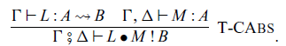
By the induction hypothesis, we have
 \begin{align*} \mathord{\left[\![{L}\right]\!]}(v_1, \dots, v_m) & \triangleleft_{A \rightsquigarrow B} L[V_1 / x_1, \dots, V_m / x_m], \\ \mathord{\left[\![{M}\right]\!]}(v_1, \dots, v_m, w_1, \dots, w_n) & \triangleleft_{A} M[V_1 / x_1, \dots, V_m / x_m, W_1 / y_1, \dots, W_n / y_n]. \end{align*}
By the definition of
 $\triangleleft_{A \rightsquigarrow B}$
, we have
$\triangleleft_{A \rightsquigarrow B}$
, we have
 \begin{align*} & \mathop{\mathrm{arr}}\nolimits(\mathord{\left[\![{M}\right]\!]}(v_1, \dots, v_m, w_1, \dots, w_n)) \mathrel{>\!\!>\!\!>} \mathord{\left[\![{L}\right]\!]}(v_1, \dots, v_m) \\ & \blacktriangleleft_B L[V_1 / x_1, \dots, V_m / x_m] \bullet M[V_1 / x_1, \dots, V_m / x_m, W_1 / y_1, \dots, W_n / y_n]. \end{align*}
We also have
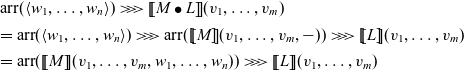 \begin{align*} & \mathop{\mathrm{arr}}\nolimits(\langle w_1 , \dots , w_n \rangle) \mathrel{>\!\!>\!\!>} \mathord{\left[\![{M \bullet L}\right]\!]}(v_1, \dots, v_m) \\ & = \mathop{\mathrm{arr}}\nolimits(\langle w_1 , \dots , w_n \rangle) \mathrel{>\!\!>\!\!>} \mathop{\mathrm{arr}}\nolimits(\mathord{\left[\![{M}\right]\!]}(v_1, \dots, v_m, {-})) \mathrel{>\!\!>\!\!>} \mathord{\left[\![{L}\right]\!]}(v_1, \dots, v_m) \\ & = \mathop{\mathrm{arr}}\nolimits(\mathord{\left[\![{M}\right]\!]}(v_1, \dots, v_m, w_1, \dots, w_n)) \mathrel{>\!\!>\!\!>} \mathord{\left[\![{L}\right]\!]}(v_1, \dots, v_m) \end{align*}
and
 \begin{align*} & (L \bullet M)[V_1 / x_1, \dots, V_m / x_m, W_1 / y_1, \dots, W_n / y_n] \\ & = L[V_1 / x_1, \dots, V_m / x_m] \bullet M[V_1 / x_1, \dots, V_m / x_m, W_1 / y_1, \dots, W_n / y_n]. \end{align*}
Therefore, we have
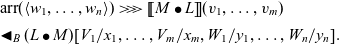 \begin{align*} & \mathop{\mathrm{arr}}\nolimits(\langle w_1 , \dots , w_n \rangle) \mathrel{>\!\!>\!\!>} \mathord{\left[\![{M \bullet L}\right]\!]}(v_1, \dots, v_m) \\ & \blacktriangleleft_B (L \bullet M)[V_1 / x_1, \dots, V_m / x_m, W_1 / y_1, \dots, W_n / y_n]. \end{align*}
In case ![]() . The derivation is
. The derivation is
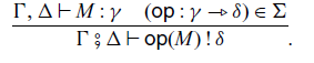
By the induction hypothesis, we have
 \begin{equation} \mathord{\left[\![{M}\right]\!]}(v_1, \dots, v_m, w_1, \dots, w_n) \triangleleft_{\gamma} M[V_1 / x_1, \dots, V_m / x_m, W_1 / y_1, \dots, W_n / y_n].\end{equation}
By the definition of
 $\triangleleft_{\delta}$
, there exists a value U such that
$\triangleleft_{\delta}$
, there exists a value U such that
 \begin{equation} M[V_1 / x_1, \dots, V_m / x_m, W_1 / y_1, \dots, W_n / y_n] \to^* U.\end{equation}
From (D1), (D2), and Lemma 5.15(1), we have
 \begin{equation} \mathord{\left[\![{M}\right]\!]}(v_1, \dots, v_m, w_1, \dots, w_n) \triangleleft_{\mathord{\left[\![{\gamma}\right]\!]}} U.\end{equation}
We have
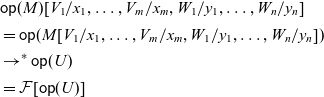 \begin{align*} & \mathsf{op}(M)[V_1 / x_1, \dots, V_m / x_m, W_1 / y_1, \dots, W_n / y_n] \\ & = \mathsf{op}(M[V_1 / x_1, \dots, V_m / x_m, W_1 / y_1, \dots, W_n / y_n]) \\ & \to^* \mathsf{op}(U) \\ & = \mathcal{F}[\mathsf{op}(U)] \end{align*}
for the trivial context
 $\mathcal{F} = [{-}]$
, and
$\mathcal{F} = [{-}]$
, and
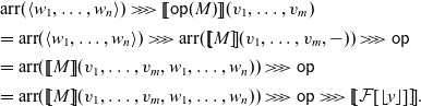 \begin{align*} & \mathop{\mathrm{arr}}\nolimits(\langle w_1, \dots, w_n \rangle) \mathrel{>\!\!>\!\!>} \mathord{\left[\![{\mathsf{op}(M)}\right]\!]}(v_1, \dots, v_m) \\ & = \mathop{\mathrm{arr}}\nolimits(\langle w_1, \dots, w_n \rangle) \mathrel{>\!\!>\!\!>} \mathop{\mathrm{arr}}\nolimits(\mathord{\left[\![{M}\right]\!]}(v_1, \dots, v_m, {-})) \mathrel{>\!\!>\!\!>} \mathsf{op} \\ & = \mathop{\mathrm{arr}}\nolimits(\mathord{\left[\![{M}\right]\!]}(v_1, \dots, v_m, w_1, \dots, w_n)) \mathrel{>\!\!>\!\!>} \mathsf{op} \\ & = \mathop{\mathrm{arr}}\nolimits(\mathord{\left[\![{M}\right]\!]}(v_1, \dots, v_m, w_1, \dots, w_n)) \mathrel{>\!\!>\!\!>} \mathsf{op} \mathrel{>\!\!>\!\!>} \mathord{\left[\![{\mathcal{F}[\lfloor{y}\rfloor]}\right]\!]}. \end{align*}
If
 $w \triangleleft_{\delta} W$
then
$w \triangleleft_{\delta} W$
then
 $\mathop{\mathrm{arr}}\nolimits(w) \blacktriangleleft_{\delta} \lfloor{W}\rfloor = \mathcal{F}[\lfloor{W}\rfloor]$
. Therefore, by the definition of
$\mathop{\mathrm{arr}}\nolimits(w) \blacktriangleleft_{\delta} \lfloor{W}\rfloor = \mathcal{F}[\lfloor{W}\rfloor]$
. Therefore, by the definition of
 $\blacktriangleleft_{\delta}$
, we have
$\blacktriangleleft_{\delta}$
, we have
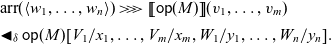 \begin{align*} & \mathop{\mathrm{arr}}\nolimits(\langle w_1, \dots, w_n \rangle) \mathrel{>\!\!>\!\!>} \mathord{\left[\![{\mathsf{op}(M)}\right]\!]}(v_1, \dots, v_m) \\ & \blacktriangleleft_{\delta} \mathsf{op}(M)[V_1 / x_1, \dots, V_m / x_m, W_1 / y_1, \dots, W_n / y_n]. \end{align*}
In case ![]() . The derivation is
. The derivation is
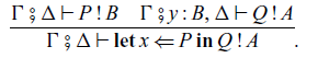
Let
 $P' = P[V_1 / x_1, \dots, V_m / x_m, W_1 / y_1, \dots, W_n / y_n]$
and
$P' = P[V_1 / x_1, \dots, V_m / x_m, W_1 / y_1, \dots, W_n / y_n]$
and
 $Q' = Q[V_1 / x_1, \dots, V_m / x_m, W_1 / y_1, \dots, W_n / y_n]$
. By the induction hypothesis, we have
$Q' = Q[V_1 / x_1, \dots, V_m / x_m, W_1 / y_1, \dots, W_n / y_n]$
. By the induction hypothesis, we have
 \begin{equation*} \mathop{\mathrm{arr}}\nolimits(\langle w_1, \dots, w_n \rangle) \mathrel{>\!\!>\!\!>} \mathord{\left[\![{P}\right]\!]}(v_1, \dots, v_m) \blacktriangleleft_A P' \end{equation*}
and
 \begin{equation*} \mathop{\mathrm{arr}}\nolimits(\langle u, w_1, \dots, w_n \rangle) \mathrel{>\!\!>\!\!>} \mathord{\left[\![{Q}\right]\!]}(v_1, \dots, v_m) \blacktriangleleft_B Q'[U/y] \end{equation*}
for any
 $u \in \mathord{\left[\![{B}\right]\!]}$
and a value U with
$u \in \mathord{\left[\![{B}\right]\!]}$
and a value U with
 $u \triangleleft_{B} U$
. By the definition of
$u \triangleleft_{B} U$
. By the definition of
 $\blacktriangleleft_{A}$
, there are two cases.
$\blacktriangleleft_{A}$
, there are two cases.
Case
 $P' \to^* \lfloor{U}\rfloor$
for a value U and there exists
$P' \to^* \lfloor{U}\rfloor$
for a value U and there exists
 $u \in \mathord{\left[\![{B}\right]\!]}$
such that
$u \in \mathord{\left[\![{B}\right]\!]}$
such that
 $\mathop{\mathrm{arr}}\nolimits(w_1, \dots, w_n) \mathrel{>\!\!>\!\!>} \mathord{\left[\![{P}\right]\!]}(v_1, \dots, v_m) = \mathop{\mathrm{arr}}\nolimits(u)$
and
$\mathop{\mathrm{arr}}\nolimits(w_1, \dots, w_n) \mathrel{>\!\!>\!\!>} \mathord{\left[\![{P}\right]\!]}(v_1, \dots, v_m) = \mathop{\mathrm{arr}}\nolimits(u)$
and
 $u \triangleleft_B U$
. We have
$u \triangleleft_B U$
. We have
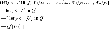 \begin{align*} & (\mathop{\mathbf{let}} y \Leftarrow P \mathop{\mathbf{in}} Q)[V_1 / x_1, \dots, V_m / x_m, W_1 / y_1, \dots, W_n / y_n] \\ & = \mathop{\mathbf{let}} y \Leftarrow P' \mathop{\mathbf{in}} Q' \\ & \to^* \mathop{\mathbf{let}} y \Leftarrow \lfloor{U}\rfloor \mathop{\mathbf{in}} Q' \\ & \to Q'[U/y] \end{align*}
and
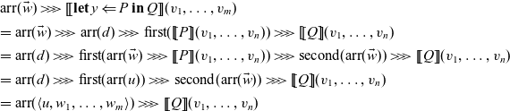 \begin{align*} & \mathop{\mathrm{arr}}\nolimits(\vec{w}) \mathrel{>\!\!>\!\!>} \mathord{\left[\![{\mathop{\mathbf{let}} y \Leftarrow P \mathop{\mathbf{in}} Q}\right]\!]}(v_1, \dots, v_m) \\ & = \mathop{\mathrm{arr}}\nolimits(\vec{w}) \mathrel{>\!\!>\!\!>} \mathop{\mathrm{arr}}\nolimits(d) \mathrel{>\!\!>\!\!>} \mathop{\mathrm{first}}\nolimits(\mathord{\left[\![{P}\right]\!]}(v_1, \dots, v_n)) \mathrel{>\!\!>\!\!>} \mathord{\left[\![{Q}\right]\!]}(v_1, \dots, v_n) \\ & = \mathop{\mathrm{arr}}\nolimits(d) \mathrel{>\!\!>\!\!>} \mathop{\mathrm{first}}\nolimits(\mathop{\mathrm{arr}}\nolimits(\vec{w}) \mathrel{>\!\!>\!\!>} \mathord{\left[\![{P}\right]\!]}(v_1, \dots, v_n)) \mathrel{>\!\!>\!\!>} \mathop{\mathrm{second}}\nolimits(\mathop{\mathrm{arr}}\nolimits(\vec{w})) \mathrel{>\!\!>\!\!>} \mathord{\left[\![{Q}\right]\!]}(v_1, \dots, v_n) \\ & = \mathop{\mathrm{arr}}\nolimits(d) \mathrel{>\!\!>\!\!>} \mathop{\mathrm{first}}\nolimits(\mathop{\mathrm{arr}}\nolimits(u)) \mathrel{>\!\!>\!\!>} \mathop{\mathrm{second}}\nolimits(\mathop{\mathrm{arr}}\nolimits(\vec{w})) \mathrel{>\!\!>\!\!>} \mathord{\left[\![{Q}\right]\!]}(v_1, \dots, v_n) \\ & = \mathop{\mathrm{arr}}\nolimits(\langle u, w_1, \dots, w_m \rangle) \mathrel{>\!\!>\!\!>} \mathord{\left[\![{Q}\right]\!]}(v_1, \dots, v_n) \end{align*}
where
 $\vec{w} = \langle w_1, \dots, w_n \rangle$
. Hence, by Lemma 5.15(3), we obtain
$\vec{w} = \langle w_1, \dots, w_n \rangle$
. Hence, by Lemma 5.15(3), we obtain
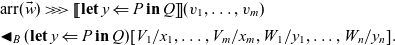 \begin{align*} & \mathop{\mathrm{arr}}\nolimits(\vec{w}) \mathrel{>\!\!>\!\!>} \mathord{\left[\![{\mathop{\mathbf{let}} y \Leftarrow P \mathop{\mathbf{in}} Q}\right]\!]}(v_1, \dots, v_m) \\ & \blacktriangleleft_B (\mathop{\mathbf{let}} y \Leftarrow P \mathop{\mathbf{in}} Q)[V_1 / x_1, \dots, V_m / x_m, W_1 / y_1, \dots, W_n / y_n]. \end{align*}
Case
 $P' \to^* \mathcal{F}[\mathsf{op}(U)]$
for a value U and
$P' \to^* \mathcal{F}[\mathsf{op}(U)]$
for a value U and ![]() and there exists
and there exists
 $u \in \mathord{\left[\![{\gamma}\right]\!]}$
with
$u \in \mathord{\left[\![{\gamma}\right]\!]}$
with
 $u \triangleleft_{\gamma} U$
and
$u \triangleleft_{\gamma} U$
and
 $b \in \mathcal{A}_{\Sigma}(\mathord{\left[\![{\delta}\right]\!]}, \mathord{\left[\![{A}\right]\!]})$
such that
$b \in \mathcal{A}_{\Sigma}(\mathord{\left[\![{\delta}\right]\!]}, \mathord{\left[\![{A}\right]\!]})$
such that
 $\mathop{\mathrm{arr}}\nolimits(\langle w_1, \dots, w_n \rangle) \mathrel{>\!\!>\!\!>} \mathord{\left[\![{P}\right]\!]}(v_1, \dots, v_m) = \mathop{\mathrm{arr}}\nolimits(u) \mathrel{>\!\!>\!\!>} \mathsf{op} \mathrel{>\!\!>\!\!>} b$
and
$\mathop{\mathrm{arr}}\nolimits(\langle w_1, \dots, w_n \rangle) \mathrel{>\!\!>\!\!>} \mathord{\left[\![{P}\right]\!]}(v_1, \dots, v_m) = \mathop{\mathrm{arr}}\nolimits(u) \mathrel{>\!\!>\!\!>} \mathsf{op} \mathrel{>\!\!>\!\!>} b$
and
 $w \triangleleft_{\delta} W \implies \mathop{\mathrm{arr}}\nolimits(w) \mathrel{>\!\!>\!\!>} b \blacktriangleleft_{A} \mathcal{F}[\lfloor{W}\rfloor]$
for any
$w \triangleleft_{\delta} W \implies \mathop{\mathrm{arr}}\nolimits(w) \mathrel{>\!\!>\!\!>} b \blacktriangleleft_{A} \mathcal{F}[\lfloor{W}\rfloor]$
for any
 $w \in \mathord{\left[\![{\delta}\right]\!]}$
and a value W. We have
$w \in \mathord{\left[\![{\delta}\right]\!]}$
and a value W. We have
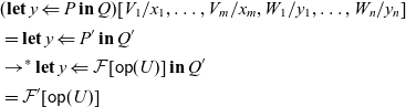 \begin{align*} & (\mathop{\mathbf{let}} y \Leftarrow P \mathop{\mathbf{in}} Q)[V_1 / x_1, \dots, V_m / x_m, W_1 / y_1, \dots, W_n / y_n] \\ & = \mathop{\mathbf{let}} y \Leftarrow P' \mathop{\mathbf{in}} Q' \\ & \to^* \mathop{\mathbf{let}} y \Leftarrow \mathcal{F}[\mathsf{op}(U)] \mathop{\mathbf{in}} Q' \\ & = \mathcal{F}'[\mathsf{op}(U)] \end{align*}
where
 $\mathcal{F}' = \mathop{\mathbf{let}} y \Leftarrow \mathcal{F} \mathop{\mathbf{in}} Q'$
, and
$\mathcal{F}' = \mathop{\mathbf{let}} y \Leftarrow \mathcal{F} \mathop{\mathbf{in}} Q'$
, and
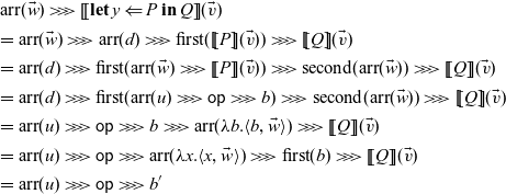 \begin{align*} & \mathop{\mathrm{arr}}\nolimits(\vec{w}) \mathrel{>\!\!>\!\!>} \mathord{\left[\![{\mathop{\mathbf{let}} y \Leftarrow P \mathop{\mathbf{in}} Q}\right]\!]}(\vec{v}) \\ & = \mathop{\mathrm{arr}}\nolimits(\vec{w}) \mathrel{>\!\!>\!\!>} \mathop{\mathrm{arr}}\nolimits(d) \mathrel{>\!\!>\!\!>} \mathop{\mathrm{first}}\nolimits(\mathord{\left[\![{P}\right]\!]}(\vec{v})) \mathrel{>\!\!>\!\!>} \mathord{\left[\![{Q}\right]\!]}(\vec{v}) \\ & = \mathop{\mathrm{arr}}\nolimits(d) \mathrel{>\!\!>\!\!>} \mathop{\mathrm{first}}\nolimits(\mathop{\mathrm{arr}}\nolimits(\vec{w}) \mathrel{>\!\!>\!\!>} \mathord{\left[\![{P}\right]\!]}(\vec{v})) \mathrel{>\!\!>\!\!>} \mathop{\mathrm{second}}\nolimits(\mathop{\mathrm{arr}}\nolimits(\vec{w})) \mathrel{>\!\!>\!\!>} \mathord{\left[\![{Q}\right]\!]}(\vec{v}) \\ & = \mathop{\mathrm{arr}}\nolimits(d) \mathrel{>\!\!>\!\!>} \mathop{\mathrm{first}}\nolimits(\mathop{\mathrm{arr}}\nolimits(u) \mathrel{>\!\!>\!\!>} \mathsf{op} \mathrel{>\!\!>\!\!>} b) \mathrel{>\!\!>\!\!>} \mathop{\mathrm{second}}\nolimits(\mathop{\mathrm{arr}}\nolimits(\vec{w})) \mathrel{>\!\!>\!\!>} \mathord{\left[\![{Q}\right]\!]}(\vec{v}) \\ & = \mathop{\mathrm{arr}}\nolimits(u) \mathrel{>\!\!>\!\!>} \mathsf{op} \mathrel{>\!\!>\!\!>} b \mathrel{>\!\!>\!\!>} \mathop{\mathrm{arr}}\nolimits(\lambda b . \langle b, \vec{w} \rangle) \mathrel{>\!\!>\!\!>} \mathord{\left[\![{Q}\right]\!]}(\vec{v}) \\ & = \mathop{\mathrm{arr}}\nolimits(u) \mathrel{>\!\!>\!\!>} \mathsf{op} \mathrel{>\!\!>\!\!>} \mathop{\mathrm{arr}}\nolimits(\lambda x . \langle x, \vec{w} \rangle) \mathrel{>\!\!>\!\!>} \mathop{\mathrm{first}}\nolimits(b) \mathrel{>\!\!>\!\!>} \mathord{\left[\![{Q}\right]\!]}(\vec{v}) \\ & = \mathop{\mathrm{arr}}\nolimits(u) \mathrel{>\!\!>\!\!>} \mathsf{op} \mathrel{>\!\!>\!\!>} b' \end{align*}
where
 $\vec{w} = \langle w_1, \dots, w_n \rangle$
,
$\vec{w} = \langle w_1, \dots, w_n \rangle$
,
 $\vec{v} = \langle v_1, \dots, v_m \rangle$
and
$\vec{v} = \langle v_1, \dots, v_m \rangle$
and
 $b' = \mathop{\mathrm{arr}}\nolimits(\lambda x . \langle x, \vec{w} \rangle) \mathrel{>\!\!>\!\!>} \mathop{\mathrm{first}}\nolimits(b) \mathrel{>\!\!>\!\!>} \mathord{\left[\![{Q}\right]\!]}(\vec{v})$
. Given
$b' = \mathop{\mathrm{arr}}\nolimits(\lambda x . \langle x, \vec{w} \rangle) \mathrel{>\!\!>\!\!>} \mathop{\mathrm{first}}\nolimits(b) \mathrel{>\!\!>\!\!>} \mathord{\left[\![{Q}\right]\!]}(\vec{v})$
. Given
 $w \in \mathord{\left[\![{\delta}\right]\!]}$
and
$w \in \mathord{\left[\![{\delta}\right]\!]}$
and
 $\diamond \vdash W : \delta$
with
$\diamond \vdash W : \delta$
with
 $w \triangleleft_{\delta} W$
, we can show
$w \triangleleft_{\delta} W$
, we can show
 $\mathop{\mathrm{arr}}\nolimits(w) \mathrel{>\!\!>\!\!>} b' \blacktriangleleft_{B} \mathcal{F}'[\lfloor{W}\rfloor]$
. Therefore, we have
$\mathop{\mathrm{arr}}\nolimits(w) \mathrel{>\!\!>\!\!>} b' \blacktriangleleft_{B} \mathcal{F}'[\lfloor{W}\rfloor]$
. Therefore, we have
 \begin{align*} & \mathop{\mathrm{arr}}\nolimits(\vec{w}) \mathrel{>\!\!>\!\!>} \mathord{\left[\![{\mathop{\mathbf{let}} y \Leftarrow P \mathop{\mathbf{in}} Q}\right]\!]}(v_1, \dots, v_m) \\ & \blacktriangleleft_B (\mathop{\mathbf{let}} y \Leftarrow P \mathop{\mathbf{in}} Q)[V_1 / x_1, \dots, V_m / x_m, W_1 / y_1, \dots, W_n / y_n]. \end{align*}
In case ![]() . The derivation is
. The derivation is
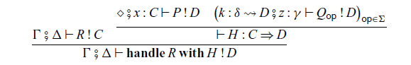
where ![]() . Let
. Let
 $R' = R[V_1 / x_1, \dots, V_m / x_m, W_1 / y_1, \dots, W_n / y_n]$
. By the induction hypothesis, we have
$R' = R[V_1 / x_1, \dots, V_m / x_m, W_1 / y_1, \dots, W_n / y_n]$
. By the induction hypothesis, we have
 \begin{equation*} \mathop{\mathrm{arr}}\nolimits(\langle w_1, \dots, w_n \rangle) \mathrel{>\!\!>\!\!>} \mathord{\left[\![{R}\right]\!]}(v_1, \dots, v_m) \blacktriangleleft_{C} R'. \end{equation*}
By the definition of
 $\blacktriangleleft_{C}$
, there are two cases.
$\blacktriangleleft_{C}$
, there are two cases.
Case
 $R' \to^* \lfloor{U}\rfloor$
for a value U and there exists
$R' \to^* \lfloor{U}\rfloor$
for a value U and there exists
 $u \in \mathord{\left[\![{C}\right]\!]}$
such that
$u \in \mathord{\left[\![{C}\right]\!]}$
such that
 $\mathop{\mathrm{arr}}\nolimits(\langle w_1, \dots, w_n \rangle) \mathrel{>\!\!>\!\!>} \mathord{\left[\![{R}\right]\!]}(v_1, \dots, v_m) = \mathop{\mathrm{arr}}\nolimits(u)$
and
$\mathop{\mathrm{arr}}\nolimits(\langle w_1, \dots, w_n \rangle) \mathrel{>\!\!>\!\!>} \mathord{\left[\![{R}\right]\!]}(v_1, \dots, v_m) = \mathop{\mathrm{arr}}\nolimits(u)$
and
 $u \triangleleft_{C} U$
. By the induction hypothesis and
$u \triangleleft_{C} U$
. By the induction hypothesis and
 $u \triangleleft_{C} U$
, we have
$u \triangleleft_{C} U$
, we have
 \begin{equation*} \mathop{\mathrm{arr}}\nolimits(u) \mathrel{>\!\!>\!\!>} \mathord{\left[\![{P}\right]\!]} \blacktriangleleft_{D} P[U/x]. \end{equation*}
We have
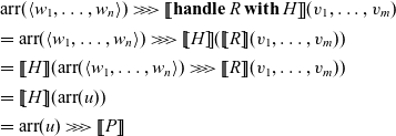 \begin{align*} & \mathop{\mathrm{arr}}\nolimits(\langle w_1, \dots, w_n \rangle) \mathrel{>\!\!>\!\!>} \mathord{\left[\![{\mathop{\mathbf{handle}} R \mathop{\mathbf{with}} H}\right]\!]}(v_1, \dots, v_m) \\ & = \mathop{\mathrm{arr}}\nolimits(\langle w_1, \dots, w_n \rangle) \mathrel{>\!\!>\!\!>} \mathord{\left[\![{H}\right]\!]}(\mathord{\left[\![{R}\right]\!]}(v_1, \dots, v_m)) \\ & = \mathord{\left[\![{H}\right]\!]}(\mathop{\mathrm{arr}}\nolimits(\langle w_1, \dots, w_n \rangle) \mathrel{>\!\!>\!\!>} \mathord{\left[\![{R}\right]\!]}(v_1, \dots, v_m)) \\ & = \mathord{\left[\![{H}\right]\!]}(\mathop{\mathrm{arr}}\nolimits(u)) \\ & = \mathop{\mathrm{arr}}\nolimits(u) \mathrel{>\!\!>\!\!>} \mathord{\left[\![{P}\right]\!]} \end{align*}
and
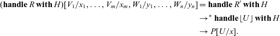 \begin{align*} (\mathop{\mathbf{handle}} R \mathop{\mathbf{with}} H)[V_1 / x_1, \dots, V_m / x_m, W_1 / y_1, \dots, W_n / y_n] & = \mathop{\mathbf{handle}} R' \mathop{\mathbf{with}} H \\ & \to^* \mathop{\mathbf{handle}} \lfloor{U}\rfloor \mathop{\mathbf{with}} H \\ & \to P[U / x]. \end{align*}
Therefore, by Lemma 5.15(3), we obtain
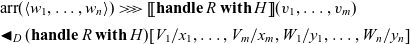 \begin{align*} & \mathop{\mathrm{arr}}\nolimits(\langle w_1, \dots, w_n \rangle) \mathrel{>\!\!>\!\!>} \mathord{\left[\![{\mathop{\mathbf{handle}} R \mathop{\mathbf{with}} H}\right]\!]}(v_1, \dots, v_m) \\ & \blacktriangleleft_{D} (\mathop{\mathbf{handle}} R \mathop{\mathbf{with}} H)[V_1 / x_1, \dots, V_m / x_m, W_1 / y_1, \dots, W_n / y_n] \end{align*}
Case
 $R' \to^* \mathcal{F}[\mathsf{op}(U)]$
for a value U and
$R' \to^* \mathcal{F}[\mathsf{op}(U)]$
for a value U and ![]() and there exist
and there exist
 $u \in \mathord{\left[\![{\gamma}\right]\!]}$
with
$u \in \mathord{\left[\![{\gamma}\right]\!]}$
with
 $u \triangleleft_{\gamma} U$
and
$u \triangleleft_{\gamma} U$
and
 $b \in \mathcal{A}_{\Sigma}(\mathord{\left[\![{\delta}\right]\!]}, \mathord{\left[\![{C}\right]\!]})$
such that
$b \in \mathcal{A}_{\Sigma}(\mathord{\left[\![{\delta}\right]\!]}, \mathord{\left[\![{C}\right]\!]})$
such that
 $\mathop{\mathrm{arr}}\nolimits(\langle w_1, \dots, w_n \rangle) \mathrel{>\!\!>\!\!>} \mathord{\left[\![{R}\right]\!]}(v_1, \dots, v_m) = \mathop{\mathrm{arr}}\nolimits(u) \mathrel{>\!\!>\!\!>} \mathsf{op} \mathrel{>\!\!>\!\!>} b$
and
$\mathop{\mathrm{arr}}\nolimits(\langle w_1, \dots, w_n \rangle) \mathrel{>\!\!>\!\!>} \mathord{\left[\![{R}\right]\!]}(v_1, \dots, v_m) = \mathop{\mathrm{arr}}\nolimits(u) \mathrel{>\!\!>\!\!>} \mathsf{op} \mathrel{>\!\!>\!\!>} b$
and
 $w \triangleleft_{\delta} W \implies \mathop{\mathrm{arr}}\nolimits(w) \mathrel{>\!\!>\!\!>} b \blacktriangleleft_{C} \mathcal{F}[\lfloor{W}\rfloor]$
for any
$w \triangleleft_{\delta} W \implies \mathop{\mathrm{arr}}\nolimits(w) \mathrel{>\!\!>\!\!>} b \blacktriangleleft_{C} \mathcal{F}[\lfloor{W}\rfloor]$
for any
 $w \in \mathord{\left[\![{\delta}\right]\!]}$
and
$w \in \mathord{\left[\![{\delta}\right]\!]}$
and
 $\diamond \vdash W : \delta$
. Let
$\diamond \vdash W : \delta$
. Let
 $Q_{\mathsf{op}}' = Q_{\mathsf{op}}[U / z, (\lambda^{\bullet} y . \mathop{\mathbf{handle}} \mathcal{F}[\lfloor{y}\rfloor] \mathop{\mathbf{with}} H) / k]$
. We have
$Q_{\mathsf{op}}' = Q_{\mathsf{op}}[U / z, (\lambda^{\bullet} y . \mathop{\mathbf{handle}} \mathcal{F}[\lfloor{y}\rfloor] \mathop{\mathbf{with}} H) / k]$
. We have
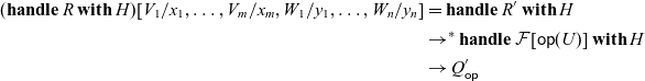 \begin{align*} (\mathop{\mathbf{handle}} R \mathop{\mathbf{with}} H)[V_1 / x_1, \dots, V_m / x_m, W_1 / y_1, \dots, W_n / y_n] & = \mathop{\mathbf{handle}} R' \mathop{\mathbf{with}} H \\ & \to^* \mathop{\mathbf{handle}} \mathcal{F}[\mathsf{op}(U)] \mathop{\mathbf{with}} H \\ & \to Q_{\mathsf{op}}' \end{align*}
By the induction hypothesis and
 $u \triangleleft_{\gamma} U$
, we have
$u \triangleleft_{\gamma} U$
, we have
 $\mathop{\mathrm{arr}}\nolimits(u) \mathrel{>\!\!>\!\!>} \mathord{\left[\![{Q_{\mathsf{op}}}\right]\!]}( \kappa ) \blacktriangleleft_{D} Q_{\mathsf{op}}'$
for any
$\mathop{\mathrm{arr}}\nolimits(u) \mathrel{>\!\!>\!\!>} \mathord{\left[\![{Q_{\mathsf{op}}}\right]\!]}( \kappa ) \blacktriangleleft_{D} Q_{\mathsf{op}}'$
for any
 $\kappa \in \mathord{\left[\![{\delta \rightsquigarrow D}\right]\!]}$
with
$\kappa \in \mathord{\left[\![{\delta \rightsquigarrow D}\right]\!]}$
with
 $\kappa \triangleleft_{\delta \rightsquigarrow D} (\lambda^{\bullet} y . \mathop{\mathbf{handle}} \mathcal{F}[\lfloor{y}\rfloor] \mathop{\mathbf{with}} H)$
. We can show
$\kappa \triangleleft_{\delta \rightsquigarrow D} (\lambda^{\bullet} y . \mathop{\mathbf{handle}} \mathcal{F}[\lfloor{y}\rfloor] \mathop{\mathbf{with}} H)$
. We can show
 $\mathord{\left[\![{H}\right]\!]}(b) \triangleleft_{\delta \rightsquigarrow D} \lambda^{\bullet} y . \mathop{\mathbf{handle}} \mathcal{F}[\lfloor{y}\rfloor] \mathop{\mathbf{with}} H$
from
$\mathord{\left[\![{H}\right]\!]}(b) \triangleleft_{\delta \rightsquigarrow D} \lambda^{\bullet} y . \mathop{\mathbf{handle}} \mathcal{F}[\lfloor{y}\rfloor] \mathop{\mathbf{with}} H$
from
 $\forall w.\ \forall W.\ w \triangleleft_{\delta} W \implies \mathop{\mathrm{arr}}\nolimits(w) \mathrel{>\!\!>\!\!>} b \blacktriangleleft_{C} \mathcal{F}[\lfloor{W}\rfloor]$
. Thus, we have
$\forall w.\ \forall W.\ w \triangleleft_{\delta} W \implies \mathop{\mathrm{arr}}\nolimits(w) \mathrel{>\!\!>\!\!>} b \blacktriangleleft_{C} \mathcal{F}[\lfloor{W}\rfloor]$
. Thus, we have
 \begin{equation*} \mathop{\mathrm{arr}}\nolimits(u) \mathrel{>\!\!>\!\!>} \mathord{\left[\![{Q_{\mathsf{op}}}\right]\!]}( \mathord{\left[\![{H}\right]\!]}(b) ) \blacktriangleleft_{D} Q_{\mathsf{op}}' \end{equation*}
By Lemma 5.15(3), we obtain
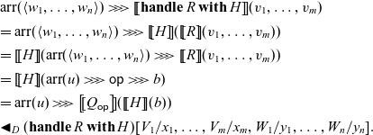 \begin{align*} & \mathop{\mathrm{arr}}\nolimits(\langle w_1, \dots, w_n \rangle) \mathrel{>\!\!>\!\!>} \mathord{\left[\![{\mathop{\mathbf{handle}} R \mathop{\mathbf{with}} H}\right]\!]}(v_1, \dots, v_m) \\ & = \mathop{\mathrm{arr}}\nolimits(\langle w_1, \dots, w_n \rangle) \mathrel{>\!\!>\!\!>} \mathord{\left[\![{H}\right]\!]}(\mathord{\left[\![{R}\right]\!]}(v_1, \dots, v_m)) \\ & = \mathord{\left[\![{H}\right]\!]}(\mathop{\mathrm{arr}}\nolimits(\langle w_1, \dots, w_n \rangle) \mathrel{>\!\!>\!\!>} \mathord{\left[\![{R}\right]\!]}(v_1, \dots, v_m)) \\ & = \mathord{\left[\![{H}\right]\!]}(\mathop{\mathrm{arr}}\nolimits(u) \mathrel{>\!\!>\!\!>} \mathsf{op} \mathrel{>\!\!>\!\!>} b) \\ & = \mathop{\mathrm{arr}}\nolimits(u) \mathrel{>\!\!>\!\!>} \mathord{\left[\![{Q_{\mathsf{op}}}\right]\!]}(\mathord{\left[\![{H}\right]\!]}(b)) \\ & \blacktriangleleft_{D} (\mathop{\mathbf{handle}} R \mathop{\mathbf{with}} H)[V_1 / x_1, \dots, V_m / x_m, W_1 / y_1, \dots, W_n / y_n]. \end{align*}
E Proofs for Section 6 (Related work)
Proposition 6.1. There is a map
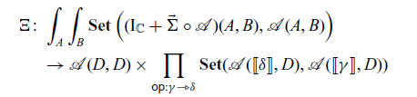
for any set D.
Proof. By the following calculation:
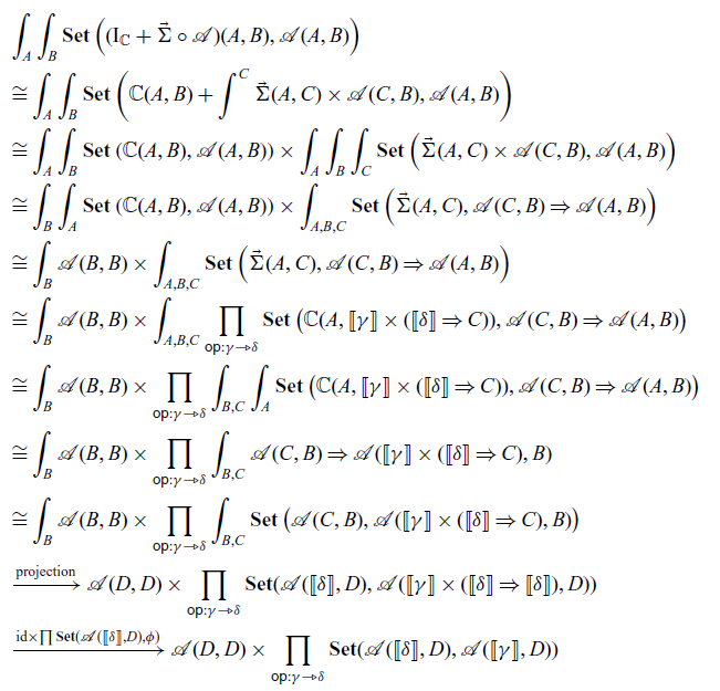
where
 $\phi \colon \mathcal{A}(\mathord{\left[\![{\gamma}\right]\!]} \times (\mathord{\left[\![{\delta}\right]\!]} \Rightarrow \mathord{\left[\![{\delta}\right]\!]}), D) \to \mathcal{A}(\mathord{\left[\![{\gamma}\right]\!]}, D)$
is defined as
$\phi \colon \mathcal{A}(\mathord{\left[\![{\gamma}\right]\!]} \times (\mathord{\left[\![{\delta}\right]\!]} \Rightarrow \mathord{\left[\![{\delta}\right]\!]}), D) \to \mathcal{A}(\mathord{\left[\![{\gamma}\right]\!]}, D)$
is defined as
 \begin{equation*} \phi(a) = \mu^{\mathcal{A}}_{\mathord{\left[\![{\gamma}\right]\!]}, \mathord{\left[\![{\gamma}\right]\!]} \times (\mathord{\left[\![{\delta}\right]\!]} \Rightarrow \mathord{\left[\![{\delta}\right]\!]}), D} \left( \eta^{\mathcal{A}}_{\mathord{\left[\![{\gamma}\right]\!]}, \mathord{\left[\![{\gamma}\right]\!]} \times (\mathord{\left[\![{\delta}\right]\!]} \Rightarrow \mathord{\left[\![{\delta}\right]\!]})}(\langle\mathrm{id}_{\mathord{\left[\![{\gamma}\right]\!]}}, \Lambda(\mathrm{id}_{\mathord{\left[\![{\delta}\right]\!]}})\rangle), a \right). \end{equation*}


 Open access
Discussions
No Discussions have been published for this article.