On the aeroelastic bifurcation of a flexible panel subjected to cavity pressure and inviscid oblique shock

Abstract

The aeroelasticity of a panel in the presence of a shock is a fundamental issue of great significance in the development of hypersonic vehicles. In practical engineering, cavity pressure emerges as a crucial factor that influences the nonlinear dynamical characteristics of the panel. This study focuses on the aeroelastic bifurcation of a flexible panel subjected to both cavity pressure and oblique shock. To this end, a computational method is devised, coupling a high-fidelity reduced-order model for unsteady aerodynamic loads with nonlinear structural equations. The solution is meticulously tracked by continuous calculations. The obtained results indicate that cavity pressure plays a pivotal role in determining the bifurcation and stability characteristics of the system. First, the system exhibits hysteresis behaviour in response to the ascending and descending dynamic pressures. The evolution of hysteresis behaviour originates from the phenomenon of cusp catastrophe. Second, variations in cavity pressure induce three types of bifurcation phenomena, exhibiting characteristics akin to supercritical Hopf bifurcation, subcritical Hopf bifurcation and saddle-node bifurcation of cycles. The system's response at the critical points of these bifurcations manifests as long-period asymptotic flutter or explosive flutter. Lastly, the evolution of the dynamical system among these three types of bifurcations is an important factor contributing to the discrepancies observed in certain research results. This study enhances the understanding of the nonlinear dynamical behaviour of panel aeroelasticity in complex practical environments and provides new explanations for the discrepancies observed in certain research results.

1. Introduction

Panel flutter, as a classic problem in the field of aeroelasticity, poses detrimental effects on the structural fatigue life, and compromises the performance and safety of vehicles. Noteworthy contributions on this matter have been made by Dowell (1970, 1974) and Mei, Abdel-Motagaly & Chen (1999), providing comprehensive reviews. In recent years, hypersonic vehicles have garnered increasing attention (Urzay 2018). Shock phenomena is one of the typical features in hypersonic flow, widely present in both internal and external flow configurations, such as the intricate shock structures found in a scramjet engine inlet (Matsuo, Miyazato & Kim 1999; Urzay 2018). The presence of shock gives rise to an accentuation of the nonlinear and unsteady characteristics of aerodynamic loads, which, in turn, lead to even greater complexity in the aeroelastic characteristics of the panel (Shinde et al. 2019; Boyer et al. 2021; Brouwer et al. 2021; He et al. 2022; Shinde, McNamara & Gaitonde 2022). Moreover, these complex aeroelastic characteristics significantly impact the performance of the vehicles (Bhattrai et al. 2022; Liu et al. 2022). Hence, the issue of panel flutter in the presence of a shock represents a fundamental problem in the development of hypersonic vehicles (McNamara & Friedmann 2011; Dowell 2015).

The aeroelasticity of the panel in the presence of a shock has been a subject of continuous interest among scholars in the past decade. Numerous preliminary explorations using numerical simulations and experimental approaches have been conducted in this area. In terms of numerical simulations, Visbal (2012) studied the aeroelasticity of a two-dimensional panel subjected to an oblique shock in inviscid flow. The study unveiled self-excited panel vibrations, and summarised the flutter characteristics and flow field structures under typical shock strengths. Notably, complex nonlinear bifurcation behaviour was observed in the dynamical system under a shock strength of 1.4. An et al. (2021) investigated the nonlinear aeroelastic responses of four curved panels of different curvature subjected to oblique shock in two-dimensional inviscid flow. The study demonstrated significant nonlinear effects, with the dynamical system exhibiting multiple solutions under different initial conditions. Transitions between these solutions were also observed. Boyer et al. (2018, 2021) extended the investigation to three-dimensional flow and found that shock strength significantly influences the stability characteristics of the panel. In comparison to inviscid flow, the presence of viscosity induces flutter dominated by higher-order modes. Shinde et al. (2019) performed a direct numerical simulation (DNS) of the shock/boundary-layer interaction on a flexible wall. The promoting effect of the flexible panel on flow transition was analysed using the proper orthogonal decomposition (POD) method. Brouwer, Gogulapati & McNamara (2017) investigated the influence of surface deformation on shock-induced separation using the Reynolds-averaged Navier–Stokes (RANS) method. Based on that study, they further developed the application of enriched piston theory in the context of shock-induced panel flutter (Brouwer & McNamara 2019). Ye & Ye (2018) conducted stability analysis, and discovered that the critical flutter dynamic pressure exhibits nonlinear and sensitive variations in response to the location of shock impingement. Li et al. (2019) investigated the inhibitory effect of surface velocity feedback control on shock-induced panel flutter in both viscous and inviscid flows. He et al. (2022) studied the aeroelastic behaviour of a panel in the presence of an irregular shock reflection and observed the onset of divergence at low dynamic pressures. In terms of experimental studies, Spottswood, Eason & Beberniss (2013), Spottswood et al. (2019) conducted a series of innovative experiments to investigate the fluid–structure interaction (FSI) behaviour of panels in shock/boundary-layer interaction under different turbulent and thermal flow conditions. Willems, Gülhan & Esser (2013) experimentally measured the deformation and vibration of panels in a shock/boundary-layer interaction and compared the results with numerical simulations. They observed that panel vibration is influenced by its static deformation component. Brouwer et al. (2021) investigated the flutter behaviour of panels in turbulent flow and a shock/boundary-layer interaction, measuring the limit cycle oscillations (LCO) induced by shock waves. Daub, Willems & Gülhan (2016) designed an experimental set-up where the unsteady shock was generated using a pitching oscillating wedge. Under the influence of high-frequency oscillating shock, a larger amplitude vibration of the panel was observed.

In practical engineering applications, the behaviour of the panel is influenced not only by unilateral aerodynamic loads, but also by the combined effect of cavity pressure underneath. Previous studies by Dowell (1966) and Visbal (2014) have demonstrated the significant impact of cavity pressure on the aeroelastic characteristics of the panel. The unbalanced cavity pressure induces additional shock/expansion wave systems, resulting in changes in the unsteady aerodynamic force characteristics (Visbal 2014; Gramola, Bruce & Santer 2020). Studies have shown that this phenomenon further enhances the nonlinear characteristics of the system. Under the absence of shock, Dowell (1966) highlighted the symmetric influence of static pressure difference on the critical dynamic pressure of flutter. Another work (Dowell 1982) reported the suppressive effect of static pressure difference on the chaotic response of buckled panels. Ye & Ye (2021) theoretically studied the stability boundary of panels in supersonic airflow using the Lyapunov method, emphasising the significant role of the coupling between static deformation and aerodynamic forces in greatly enhancing the aeroelastic stability of the panel. Under the presence of shock, Visbal (2014) conducted preliminary research on three different cavity pressure cases in inviscid flow, and the results indicated that the variation of cavity pressure has a significant impact on the characteristics of the dynamical system. Experimental findings by Spottswood et al. (2019) revealed that the dynamical characteristics of the panel are highly sensitive to sudden changes in cavity pressure. However, due to the inherent limitations of the experiment, drawing mechanistic conclusions becomes challenging. Gramola et al. (2020) found through experiments that cavity pressure significantly alters the deformation of the panel, thereby affecting the flow field structure. However, the study does not address the dynamic behaviour of the panel. Liu et al. (2022) investigated the aeroelastic behaviour of the panel in an isolator under different cavity pressures using the URANS method. Their findings indicated a significant influence of cavity pressure on the motion of shock trains and the unsteady aerodynamic characteristics. Brouwer et al. (2021, 2022) examined the influence of the shock/boundary-layer interaction on the flutter characteristics of the panel through experiments and enriched piston theory. The advanced experiment unveiled that even subtle variations in cavity pressure exhibit intricate nonlinear effects on the aeroelastic system of the panel subjected to an oblique shock. The vibration characteristics of the panel exhibited disparities with the cavity pressure increasing or decreasing.

In summary, cavity pressure plays a pivotal role in modulating the aeroelastic characteristics of the panel subjected to an oblique shock. Presently, ongoing research has identified three primary configurations concerning the cavity pressure underneath the panel: (1) average pressure on the upper surface (e.g. Visbal 2012; Li et al. 2019; An et al. 2021); (2) pressure distribution that maintains zero initial static pressure difference (e.g. Ye & Ye 2018; He et al. 2022); (3) specific pressure value (e.g. Visbal 2014; Daub et al. 2016; Gramola et al. 2020; Brouwer et al. 2021, 2022). These studies demonstrate that the aeroelastic system of the panel subjected to both cavity pressure and oblique shock exhibits rich nonlinear behaviour. A certain level of cavity pressure can either enhance the stability boundary, thereby suppressing instability (e.g. Visbal 2014), or alter the characteristics of the system, leading to complex bifurcation and chaotic phenomena (e.g. Brouwer et al. 2021). However, the current research on this issue is still in its early stages, and the underlying mechanisms through which cavity pressure affects this dynamical system are not yet fully understood.

To examine the nonlinear dynamical behaviour and mechanisms of a panel subjected to both cavity pressure and inviscid oblique shock, a reduced-order model (ROM) for unsteady aerodynamic loads based on computational fluid dynamics (CFD) is established. Then, an FSI analysis method is developed by coupling computational structure dynamics (CSD). The calculations consider the variation of non-dimensional dynamic pressure in both ascending and descending directions, and the tracking of solutions is achieved through continuous parameter variation. The study investigates the aeroelastic system of the panel subjected to both cavity pressure and inviscid oblique shock, exploring hysteresis behaviour, catastrophe phenomena and bifurcation characteristics.

2. Physical model

The computational model is depicted in figure 1. A two-dimensional flexible panel is embedded in a rigid plane with simple supports at both ends, i.e. no deflection and zero-moment conditions. The free stream of Mach 2 is parallel to the rigid plane. The structural parameters are consistent with those of Visbal (2012) and Gordnier & Visbal (2002). The midpoint of the flexible panel is subjected to an oblique shock. The incident and reflected shocks divide the flow region into three parts, with pressure denoted as $p_{1}$, $p_{2}$ and $p_{3}$, respectively, where $p_{1} = p_{\infty }$. This study represents the shock strength by the pressure ratio of $p_{3}/p_{1}$, which corresponds to the inviscid shock reflection on the rigid plate. This definition aligns with those presented by Visbal (2012) and Brouwer & McNamara (2019). The pressure inside the cavity underneath the panel is denoted as $p_{c}$. The present study investigates the nonlinear dynamical behaviour of the panel under different cavity pressures and incoming dynamic pressures for the case of $p_{3}/p_{1} = 1.4$. During the vibration of the panel, the cavity pressure is assumed to be constant. It means that the cavity pressure is manifested through the pressure difference across the panel. This study does not consider the dynamic changes in cavity pressure caused by the motion of the panel.

Figure 1. Schematic of a panel subjected to both cavity pressure and oblique shock.

3. Numerical method

The calculation framework in this study, as shown in figure 2, mainly consists of three parts: the calculation of structural deformation (see § 3.1), the calculation of aerodynamic loads (see § 3.2) and the time marching method that couples the two (see § 3.3).

Figure 2. Aeroelastic calculation framework.

3.1. Calculation method for structural deformations

The von Kármán large deformation equation is solved by using Galerkin's method, which serves as the computational structure dynamics module in this study. Considering a one-dimensional isotropic flat plate, the upper surface of the panel is subjected to unsteady aerodynamic load $p$, while the lower surface is exposed to a constant cavity pressure $p_{c}$. Following the approaches outlined by Dowell (1966), Gordnier & Visbal (2002) and Visbal (2012), the equation of motion for the panel is derived based on Hamilton's principle and von Kármán large deformation theory as

(3.1)\begin{equation} \rho h \frac{\partial^2 w}{\partial t^2} + D \frac{\partial^4 w}{\partial x^4} -(N_0+N_x)\frac{\partial^2 w}{\partial x^2} +\Delta p = 0, \end{equation}

where

(3.2a)\begin{gather} D = \frac{E h^3}{12(1-\nu^2)}, \end{gather}

(3.2b)\begin{gather}N_x = \frac{E h}{2l(1-\nu^2)} \int_{0}^{l} \left( \frac{\partial w}{\partial x} \right)^2 \mathrm{d}\kern 0.06em x = 6 \frac{D}{h^2 l} \int_{0}^{l} \left( \frac{\partial w}{\partial x} \right)^2 \mathrm{d}\kern 0.06em x , \end{gather}

(3.2c)\begin{gather}\Delta p = p - p_{c} , \end{gather}

where $D$ is plate stiffness, $N_x$ is applied in-plane force, and $\Delta p$ represents the pressure difference between the upper and lower surfaces of the panel. See the nomenclature (Appendix G) for definitions of the other symbols. To simplify the equations, the following non-dimensional parameters are introduced:

(3.3a)\begin{gather} W \equiv \frac{w}{h} ,\quad \xi \equiv \frac{x}{l} ,\quad \tau \equiv t \sqrt{\frac{D}{\rho h l^4}} , \end{gather}

(3.3b)\begin{gather}\overline{\Delta p} \equiv \frac{l^4}{Dh} \Delta p ,\quad \lambda \equiv \frac{2 l^3}{D\beta} q_\infty ,\quad \beta \equiv \sqrt{M^2-1} , \end{gather}

(3.3c)\begin{gather}R_0 \equiv \frac{l^2}{D} N_0 ,\quad R_x \equiv \frac{l^2}{D} N_x . \end{gather}

By substituting the aforementioned non-dimensional parameters, (3.1) can be written as

(3.4)\begin{equation} \frac{\partial^2 W}{\partial \tau^2} + \frac{\partial^4 W}{\partial \xi^4} -(R_0+R_x)\frac{\partial^2 W}{\partial \xi^2} +\overline{\Delta p} = 0. \end{equation}

Equation (3.4) is discretised into ordinary differential equations by the use of Galerkin's method. According to the simply supported boundary condition, the non-dimensional displacement of the panel, denoted as $W$, satisfies

(3.5) \begin{equation} W(\xi,\tau) = \sum_{i=1}^{\infty}[ q_{i}(\tau) \sin(i{\rm \pi} \xi)], \end{equation}

where $q_i$ is the $i$th generalised displacement and $\sin (i{\rm \pi} \xi )$ is the $i$th mode. Substituting (3.5) into (3.4) and multiplying both sides of the equation by $\sin (n{\rm \pi} \xi )$, by using the orthogonality of the mode shapes, we can integrate both sides of the equation over the panel length, resulting in

(3.6) \begin{align} &\frac{\mathrm{d}^2q_{n}}{\mathrm{d}\tau^2} + \left( (n{\rm \pi} )^4 +R_0(n{\rm \pi} )^2 +3(n{\rm \pi} )^2\sum_{i=1}^{N_{{\textit{mode}}}}(i{\rm \pi} q_{i})^2 \right)q_{n}\nonumber\\ &\quad + 2 \underbrace{\int_{0}^{1}(\overline{\Delta p} \sin(n{\rm \pi} \xi))\,\mathrm{d}\xi}_\mathit{aerodynamic\ term} = 0. \end{align}

Here we consider that the deformation of the panel is mainly composed of the superposition of the first $N_{mode}$ modes, i.e. $n = 1, 2, \ldots, N_{mode}$. Based on the experience from Dowell (1966) and Visbal (2012), this study considers $N_{mode} = 6$.

Expanding the last term in (3.6), and introducing pressure coefficient $C_{p} \equiv (p-p_\infty )/q_\infty$ and cavity pressure coefficient $C_{pc} \equiv {p_{c}}/{p_\infty }$, we obtain

(3.7) \begin{align} &\int_{0}^{1}(\overline{\Delta p} \sin(n{\rm \pi} \xi))\,\mathrm{d}\xi\nonumber\\ &\quad=\int_{0}^{1}\left(\frac{l^4}{Dh}(p-p_{c}) \sin(n{\rm \pi} \xi)\right)\mathrm{d}\xi\nonumber\\ &\quad=\lambda \frac{l}{2 h} \beta \Biggl( \underbrace{\int_{0}^{1}(C_{p} \sin(n{\rm \pi} \xi))\,\mathrm{d}\xi}_{\mathit{generalised\ aerodynamic\ force}} - \frac{2}{\gamma M^2} \underbrace{\frac{1-\cos(n{\rm \pi} )}{n{\rm \pi} }(C_{pc}-1)}_{\mathit{cavity\ pressure\ term}} \Biggr). \end{align}

The generalised aerodynamic force (Lucia, Beran & Silva 2004) is defined as

(3.8)\begin{equation} f_{n} \equiv \int_{0}^{1}(C_{p} \sin(n{\rm \pi} \xi))\,\mathrm{d}\xi. \end{equation}

By introducing the state variable $\boldsymbol {e} = \{q_{1}, q_{2}, \ldots, q_{{N_{mode}}}, \dot {q}_{1}, \dot {q}_{2}, \ldots, \dot {q}_{{N_{mode}}}\}^{\mathrm {T}}$, and combining (3.6), the nonlinear dynamics equations of the panel can be rewritten as

(3.9) \begin{equation} \left.\begin{aligned} \frac{\mathrm{d}{e}_{{n}}}{\mathrm{d} \tau} & = e_{{n+N_{mode}}} ,\\ \frac{\mathrm{d}{e}_{{n+N_{mode}}}}{\mathrm{d} \tau} & ={-} \left( (n{\rm \pi} )^4 +R_0(n{\rm \pi} )^2 +3(n{\rm \pi} )^2\sum_{i=1}^{N_{mode}}(i{\rm \pi} e_{i})^2 \right) e_{n} \\ & \quad - \lambda \frac{l}{h} \beta \left(f_{n} -\frac{2}{\gamma M^2} \frac{1-\cos(n{\rm \pi} )}{n{\rm \pi} }(C_{pc}-1) \right) . \end{aligned}\right\} \end{equation}

According to the general framework for dynamical systems, the equivalent system of (3.9) is

(3.10)\begin{equation} \dot{\boldsymbol{e}} = \mathcal{F}(\boldsymbol{e},\boldsymbol{f}), \end{equation}

where $\boldsymbol {e}$ is the vector of state variable and $\boldsymbol {f}$ is the vector of generalised aerodynamic force.

3.2. Calculation method for aerodynamic loads

3.2.1. Computational fluid dynamics method

The Euler equations described by the arbitrary Lagrangian–Eulerian (ALE) method are solved in this study using a verified in-house code (Ye et al. 2022). The cell-centred finite-volume method is applied to solve the above governing equations. The main numerical methods are as follows. The improved advection upstream splitting method (AUSM$^+$) is used to derive the convective flux. The implicit dual time-stepping (DTS) method is employed for time marching, and the lower–upper symmetric Gauss–Seidel (LU-SGS) algorithm is used in the iteration of the pseudo-time step. In terms of boundary conditions, the free-slip boundary condition is applied at the wall, and the non-reflecting boundary condition is applied at the far field.

3.2.2. Reduced-order model for unsteady aerodynamic loads

To improve the calculation efficiency, a reduced-order model for unsteady aerodynamic loads based on the AutoRegressive with eXogenous input (ARX) model (Gao & Zhang 2020; Ye et al. 2022) is established through the system identification technique. The ARX model for a multi-input multi-output system can be given by

(3.11)\begin{equation} \boldsymbol{y}^{[k]} =\sum_{i=1}^{n_a} \boldsymbol{\mathsf{A}}_i\, \boldsymbol{y}^{[k-i]} + \sum_{i=0}^{n_b-1} \boldsymbol{\mathsf{B}}_i\, \boldsymbol{u}^{[k-i]} +\boldsymbol{e}^{[k]} , \end{equation}

where $\boldsymbol {y}^{[k]}$ and $\boldsymbol {u}^{[k]}$ are the output and input in the $k$th observation, respectively; $\boldsymbol {e}^{[k]}$ is the noise in the $k$th observation; $\boldsymbol{\mathsf{A}}_i$ and $\boldsymbol{\mathsf{B}}_i$ are the parameter matrices to be identified; and $n_a$ and $n_b$ are the order of output and input terms, respectively, which are hyper-parameters of the model.

For the specific issue in this study, we have

(3.12a,b)\begin{equation} \boldsymbol{y}^{[k]} = \{\,f_{1}^{[k]}, f_{2}^{[k]}, \ldots, f_{{N_{mode}}}^{[k]}\}^{\mathrm{T}} ,\quad \boldsymbol{u}^{[k]} = \{q_{1}^{[k]}, q_{2}^{[k]}, \ldots, q_{{N_{mode}}}^{[k]}\}^{\mathrm{T}} . \end{equation}

An appropriate training signal ($\boldsymbol {u}$ series) should be designed based on prior knowledge, and the corresponding response signal ($\kern 1.5pt \boldsymbol {y}$ series) can be obtained by CFD/CSD computations. The parameter matrices $\boldsymbol{\mathsf{A}}_i$ and $\boldsymbol{\mathsf{B}}_i$ will be determined through the least squares method using these training data, i.e. $\boldsymbol {u}$ series and $\boldsymbol {y}$ series (Gao & Zhang 2020).

3.3. Time marching method for aeroelastic equations

In this study, an improved Runge–Kutta method, as proposed by Zhang, Jiang & Ye (2007), is employed to solve (3.9). This method uses a third-order Lagrange polynomial interpolation for the aerodynamic forces, offering both efficiency and robustness. Combining with (3.10), the specific marching steps are given by

(3.13)\begin{gather} \boldsymbol{e}^{[n+1]} = \boldsymbol{e}^{[n]} + \Delta \tau (\boldsymbol{k_{1}}+2\boldsymbol{k_{2}}+2\boldsymbol{k_{3}}+\boldsymbol{k_{4}}) / 6, \end{gather}

(3.14)\begin{gather}\left.\begin{array}{c@{}} \boldsymbol{k_{1}} = \mathcal{F} ( \boldsymbol{e}^{[n]}, \quad \boldsymbol{f}^{[n]}) ,\\ \boldsymbol{k_{2}} = \mathcal{F} ( \boldsymbol{e}^{[n]}+\Delta \tau\,\boldsymbol{k_{1}}/2, \quad \boldsymbol{f}^{[n+0.5]}),\\ \boldsymbol{k_{3}} = \mathcal{F} (\boldsymbol{e}^{[n]}+\Delta \tau\,\boldsymbol{k_{2}}/2, \quad \boldsymbol{f}^{[n+0.5]}),\\ \boldsymbol{k_{4}} = \mathcal{F} (\boldsymbol{e}^{[n]}+\Delta \tau\,\boldsymbol{k_{3}}, \quad \boldsymbol{f}^{[n+1]}) , \end{array}\right\} \end{gather}

(3.15)\begin{gather}\left.\begin{array}{c@{}} \boldsymbol{f}^{[n+1]} = (4\,\boldsymbol{f}^{[n]} -6\,\boldsymbol{f}^{[n-1]} +4\,\boldsymbol{f}^{[n-2]} -\boldsymbol{f}^{[n-3]}) ,\\ \boldsymbol{f}^{[n+0.5]} = (35\,\boldsymbol{f}^{[n]} -35\,\boldsymbol{f}^{[n-1]} +21\,\boldsymbol{f}^{[n-2]} -5\,\boldsymbol{f}^{[n-3]})/16. \end{array}\right\} \end{gather}

4. Computational configuration

4.1. Computational model

Figure 3 presents the grid and corresponding boundary conditions used in the CFD simulation. This study does not involve the calculation of flow in the boundary layer, but for computational accuracy and grid deformation considerations, the grid near the panel has been appropriately refined. The shock is generated through a designed wedge, with a shock strength of $p_{3}/p_{1} = 1.4$. The compression surface of the wedge is extended appropriately to ensure that the expansion fan behind the wedge does not affect the load on the flexible panel. Figure 4 presents the contour of the density gradient in the initial flow field. The positions of the shock and expansion waves in the initial flow field are consistent with the scope of this study.

Figure 3. Computational grid and boundary conditions.

Figure 4. Contour of the density gradient in the initial flow field.

4.2. Establishment of the reduced-order model for unsteady aerodynamic loads

The main source of time cost in this study is the prediction of complex unsteady aerodynamic loads. A reduced-order model for unsteady aerodynamic loads is established based on the ARX model (Sjöberg et al. 1995; Raveh 2004; Gao et al. 2017), which possesses the advantages of simple form and efficient computation.

Figure 5(a) shows the training signals of generalised displacement used to drive the forced vibration. A sweeping signal with a wide frequency range is employed as the training signal (Gao et al. 2017), with a length of 3000 and a sampling frequency of 4000 ${\tau }^{-1}$. Figure 6 displays the power spectral density (PSD) of the training signals, covering the main frequencies of the actual CFD/CSD response (Ljung 1999). Figure 5(b) presents the generalised aerodynamic forces obtained through CFD/CSD computations for each mode of the panel under the excitation of the training signals.

Figure 5. Training data for the unsteady aerodynamic model: (a) training signals and (b) generalised aerodynamic forces.

Figure 6. Power spectral density of training signals.

Determining the hyperparameters, namely $n_a$ and $n_b$, is pivotal in the process of model establishment. For the problem addressed in this study, with a Mach number of 2, preliminary calculations indicated no subsonic conditions in the flow field at any given moment. This implies that disturbances from the structure to the flow field can only propagate downstream within the Mach cone at the disturbance location. However, for a finite-length plate, the duration of this disturbance's impact on the generalised aerodynamic forces of the panel is also finite. In other words, the generalised aerodynamic forces at any given moment should be determined by the unsteady effects of structural disturbances over a finite period, along with the unsteady flow itself. In the case of the supersonic flow investigated in this study, the inherent unsteady effects of the flow are notably weak. This is evident in the response to forced vibrations (see figure 5): the aerodynamic force stabilises rapidly after the cessation of displacement input. Hence, for this problem, it can be approximately considered that the generalised forces are dominated by the generalised displacements, i.e. the current generalised force is independent of past generalised forces. The model's parameter $n_a$ characterises the intrinsic unsteady effects of flow, while $n_b$ characterises the structural disturbances’ unsteady effects on the flow. Based on the above analysis, $n_a$ can be assumed as 0, while $n_b$ should be assigned an appropriate value. To ascertain the optimal value of $n_b$, we construct models with different $n_b$ values and assess the corresponding modelling errors. A comparative analysis of these errors enables us to determine the most suitable $n_b$ value. The modelling error, as defined by (4.1), quantifies the extent to which the model accurately captures the training generalised aerodynamic forces (Ye et al. 2022):

(4.1)\begin{equation} \boldsymbol{e}_{model} = \frac{{\displaystyle \sum_{i=1}^{N}}|\, \hat{\boldsymbol{f}}^{[i]}-\boldsymbol{f}^{[i]} | } {{\displaystyle \sum_{i=1}^{N}}| \boldsymbol{f}^{[i]} |} . \end{equation}

Figure 7 presents the variation of normalised modelling errors versus different values of $n_b$. The modelling errors of individual modal orders are normalised using their maximum and minimum values. It can be observed that the range of $n_b$ between 60 and 140 exhibits favourable error performance. Additionally, a comparison with the CFD/CSD results demonstrates that the model displays enhanced robustness when $n_b$ is set to 60, resulting in a strong agreement between the predicted values of the reduced-order model and the actual CFD/CSD results. Table 1 provides the modelling errors, root mean square errors (RMSEs) and $R^2$ scores for the case of $n_a=0$ and $n_b=60$. In this case, the model is equivalent to the Volterra model or Wiener filter (Silva 1993; Raveh 2001; Silva 2005; Balajewicz & Dowell 2012). Further evaluation of the model is detailed in Appendix C.

Figure 7. Normalised modelling error versus $n_b$.

Table 1. Modelling error.

5. Stability analysis of fixed points

Non-equilibrium cavity pressure significantly influences the fixed point (i.e. the static equilibrium position of the panel) (see Dowell 1966; Visbal 2014). However, conventional numerical simulation methods based on CFD/CSD are limited to detecting stable fixed points. The analysis of unstable fixed points relies more on theoretical methods, which further require the existence of analytic expressions (see Ye & Ye 2018). The reduced-order model established in § 4.2 provides a pathway for establishing a theoretical analysis framework based on CFD/CSD.

5.1. Static deformation characteristics

The static aerodynamic force expression is derived from the reduced order model. For (3.11), considering a static process, we have $\boldsymbol {y}^{[k]} = \boldsymbol {y}^{[k-1]} = \cdots = \boldsymbol {y}^{[k-n_a]}$, $\boldsymbol {u}^{[k]} = \boldsymbol {u}^{[k-1]} = \cdots = \boldsymbol {u}^{[k-n_b+1]}$. Thus, the static aerodynamic force can be simplified as

(5.1)\begin{equation} \tilde{\boldsymbol{y}} = (( \boldsymbol{\mathsf{I}} - \tilde{\boldsymbol{\mathsf{A}}} )^{^{{-}1}} \tilde{\boldsymbol{\mathsf{B}}}) \tilde{\boldsymbol{u}} , \end{equation}

where $\tilde {\boldsymbol{\mathsf{A}}} = \sum _{i=1}^{n_a} \boldsymbol{\mathsf{A}}_i$, $\tilde {\boldsymbol{\mathsf{B}}} = \sum _{i=0}^{n_b-1} \boldsymbol{\mathsf{B}}_i$, $\tilde {\boldsymbol {u}}$ is the generalised displacement vector of the panel with static deformation, while $\tilde {\boldsymbol {y}}$ is the generalised aerodynamic force under the static deformation.

For the structural equation, setting the time derivative of the left-hand side of (3.9) to zero yields the static structural equation as $\mathcal {F}(\boldsymbol {e},\boldsymbol {f}) = 0$, where $\boldsymbol {f}$ can be given by (5.1) as

(5.2)\begin{equation} \boldsymbol{f} = (( \boldsymbol{\mathsf{I}} - \tilde{\boldsymbol{\mathsf{A}}})^{^{{-}1}} \tilde{\boldsymbol{\mathsf{B}}}) \boldsymbol{e} + \boldsymbol{f}_0 , \end{equation}

where $\boldsymbol {f_0}$ is a constant vector related to the training of the reduced-order model (Gao et al. 2017). Note that (5.2) stands as an explicit expression. Therefore, within the equation $\mathcal {F} = 0$, $\mathcal {F}$ is a function dependent solely on $\boldsymbol {e}$. We term this equation derived from the reduced-order model as the static aeroelastic equation based on ROM. This study employs the trust region method (see Moré & Sorensen 1983) to solve this nonlinear equation with multiple inputs and outputs, considering various cavity pressures and dynamic pressures.

Figure 8(a) presents the deformations of the panel at several cavity pressures when $\lambda = 300$. Even at this relatively low dynamic pressure, CFD/CSD computations are capable of capturing these stable fixed points. The results obtained from both methods are in excellent agreement. Furthermore, figure 8(b) provides a bar graph of generalised displacements, with the transparent blue plane representing the zero plane. The first generalised displacement exhibits evident variations with cavity pressure. Overall, the deformations are primarily attributed to the contributions from the first three generalised displacements. The proportion of the first mode increases rapidly and dominates as the cavity pressure deviates further from the mean pressure. Figure 9 illustrates the variations of the first three generalised displacements with cavity pressure, indicating larger dynamic pressures induce greater changes. It is noteworthy that the second generalised displacement displays non-monotonic variations, with its maximum values exhibiting nonlinear changes with dynamic pressure, while the cavity pressures corresponding to the maximum values generally exhibit linear changes with dynamic pressure.

Figure 8. (a) Plate deformations and (b) bar graph of generalised displacements with $\lambda = 300$.

Figure 9. First three generalised displacements versus cavity pressure.

5.2. Linear stability of fixed points

Note that the calculations in § 5.1 demonstrate the existence of fixed point solutions under a wide range of cavity pressures and dynamic pressures. This section will examine the stability of these fixed points.

To begin, an analytic expression for the aeroelastic system is established. Following the procedures outlined in Appendix D, a state-space model corresponding to the aerodynamic reduced-order model can be obtained. Combining this model with the structural equation, i.e. (3.10), leads to

(5.3)\begin{equation} \left.\begin{array}{c} \dot{\boldsymbol{e}} = \mathcal{F} (\boldsymbol{e}, \boldsymbol{f} ), \\ \dot{\boldsymbol{x}} = \mathcal{G} (\boldsymbol{x}, \boldsymbol{e} ) , \end{array}\right\} \end{equation}

where

(5.4a,b)\begin{equation} \boldsymbol{f}(\boldsymbol{x},\boldsymbol{e}) = \boldsymbol{\mathsf{C}}_c \boldsymbol{x} + \{\boldsymbol{\mathsf{D}}_c \ \boldsymbol{\mathsf{O}} \} \boldsymbol{\cdot} \boldsymbol{e} + \boldsymbol{f}_0 , \quad \mathcal{G}(\boldsymbol{x},\boldsymbol{e}) = \boldsymbol{\mathsf{A}}_c \ \boldsymbol{x} + \{\boldsymbol{\mathsf{B}}_c \boldsymbol{\mathsf{O}} \} \boldsymbol{\cdot} \boldsymbol{e} , \end{equation}

correspond to the output equation and state equation of the state-space model, respectively. A similar coupling method is also adopted by Gao et al. (2017), Silva & Bartels (2004) and Ye et al. (2022). Let the state variables be denoted as $\boldsymbol {r} = \{ \boldsymbol {e},\boldsymbol {x} \}$. The aeroelastic equation, denoted as (5.3), can be expressed as $\dot {\boldsymbol {r}} = \mathcal {H}( \boldsymbol {r})$. Linearising the system at its fixed points, the Jacobian matrix is given by

(5.5) \begin{equation} \boldsymbol{\mathsf{J}} =\left\{\begin{array}{ccc} \boldsymbol{\mathsf{I}} & \boldsymbol{\mathsf{O}} & \boldsymbol{\mathsf{O}} \\ \boldsymbol{\mathsf{E}}-\lambda\displaystyle\dfrac{l}{h}\beta\ \boldsymbol{\mathsf{D}}_c & \boldsymbol{\mathsf{O}} & -\lambda\displaystyle\dfrac{l}{h}\beta\ \boldsymbol{\mathsf{C}}_c \\ \boldsymbol{\mathsf{B}}_c & \boldsymbol{\mathsf{O}} & \boldsymbol{\mathsf{A}}_c \end{array}\right\}. \end{equation}

The elements of the matrix $\boldsymbol{\mathsf{E}}$ are

(5.6) \begin{equation} \boldsymbol{\mathsf{E}}_{ij} =\left\{\begin{array}{ll} -6 (i{\rm \pi} )^2 (j{\rm \pi} )^2 q_{{0,i}} q_{{0,j}} & \mathrm{if} \ i \ne j ,\\ -(i{\rm \pi} )^4(1+9q_{{0,i}}^2) - R_0(i{\rm \pi} )^2 \displaystyle -3(i{\rm \pi} )^2\sum_{n=1,n \ne i}^{N_{mode}} (n {\rm \pi} q_{{0,n}})^2 & \mathrm{if} \ i = j , \end{array}\right. \end{equation}

where $q_{{0,i}}$ is the $i$th generalised displacement of the fixed point under corresponding cavity pressure and dynamic pressure, which has been calculated in § 5.1. Examining the eigenvalues $\varOmega$ of the matrix $\boldsymbol{\mathsf{J}}$ at each fixed point, any $\mathrm {Real}\ \varOmega _i > 0$ signifies an unstable fixed point; otherwise, it is deemed stable (see Khalil 2002, chap. 4).

Figure 10 presents the stability of the fixed points. The influence of cavity pressure on stability does not exhibit symmetric distribution about the mean pressure, differing notably from the case of a free stream condition (see Dowell 1966; Gordnier & Visbal 2002). For cases where the cavity pressure is less than the mean pressure, all fixed points are stable. The unstable region is mainly concentrated in the $C_{pc} > 1.208$ range, where the critical value exhibits a significant slope. This implies that cavity pressures below this threshold significantly enhance the stability of the panel with static deformation. The important threshold of $C_{pc}=1.208$ will be referenced frequently in subsequent discussions. The minimum critical dynamic pressure appears at approximately $C_{pc} = 1.215$. Furthermore, after $C_{pc} > 1.248$, the unstable region disappears. In other words, fixed points can be unstable only when $1.208 < C_{pc} < 1.248$; otherwise, the panel always has a stable static deformation solution. This leads to two changes in the stability of the system as the cavity pressure varies.

Figure 10. Stability of fixed points in the $\lambda - C_{pc}$ plane.

5.3. Stability from the perspective of energy transfer

The findings in § 5.2 indicate that fixed points become unstable only under limited cavity pressure for a certain dynamic pressure. The stability characteristics of FSI systems are fundamentally governed by the energy transfer between the fluid and the structure. From an energy perspective, numerous scholars have investigated the stability of FSI systems (Morse & Williamson 2009; Zhu, Su & Breuer 2020; Menon & Mittal 2021; Cheng et al. 2023).

The energy extracted from the flow to the flexible panel over a cycle can be expressed as

(5.7)\begin{equation} E^*(\tau) = \int_{\tau-\Delta\tau}^{\tau} \int_{0}^{l} (p_{c}-p) \dot{w} \, \mathrm{d}\kern 0.06em x \, \mathrm{d}\tau . \end{equation}

Using the non-dimensionalisation procedure detailed in § 3.1 and substituting the definition of generalised aerodynamic forces (3.8), we have

(5.8)\begin{align} E^*(\tau) &= h l \sum_{i=1}^{N_{mode}} \int_{\tau-\Delta\tau}^{\tau} \int_{0}^{1} (p_{c}-p) \sin(i{\rm \pi} \xi)\dot{q_i} \, \mathrm{d}\xi \, \mathrm{d}\tau\nonumber\\ &=\lambda \frac{D h}{2l^2} \beta \sum_{i=1}^{N_{mode}} \int_{\tau-\Delta\tau}^{\tau} \left( \frac{2}{\gamma M^2} {\frac{1-\cos(i{\rm \pi} )}{i{\rm \pi} }(C_{pc}-1)} -f_i \right) \dot{q_i} \, \mathrm{d}\tau . \end{align}

Note that there is no damping term in the structural equation (3.9), thus, the sign of $E^*$ directly indicates the amplification or suppression of oscillation amplitude (Cheng et al. 2023).

We investigated three cases with $C_{pc} = 1.2$, 1.23 and 1.25 corresponding to the unstable fixed point and two stable fixed points on either side, as shown in figure 10. CFD/CSD calculations are performed under specific initial conditions. For the unstable fixed point, the panel is released from the fixed point position. For the stable fixed points, the panel is displaced from their fixed point positions and then released (with a negative offset of 10 % in the second generalised displacement $q_2$). Figure 11 illustrates the energy transfer at these three fixed points. When the cavity pressure is low ($C_{pc} = 1.2$, blue line), the additional energy input from displacing the fixed point causes $E^*$ to fluctuate around 0 initially, and quickly tends to 0 over time, indicating an equilibrium energy transfer between the flow and the structure (Cheng et al. 2023). Considering the total energy transfer over time 0 to 1, we have $\int _{0}^{1} E^* \,\mathrm {d}\tau < 0$, which means the structure releases energy to the flow. This energy dissipation causes structural vibration decay and tends towards the fixed point, corresponding to the stable region in figure 10. As the cavity pressure increases to the unstable region ($C_{pc} = 1.23$, red line), a significant reversal in the direction of energy transfer occurs. It can be observed that $E^*$ diverges towards the positive half-axis during oscillations, with $\int _{0}^{1} E^* \,\mathrm {d}\tau > 0$. This indicates that the structure periodically absorbs energy from the flow, with increasing absorption, preventing the structure from stabilising at the fixed point. With further increase in cavity pressure ($C_{pc} = 1.25$, green line), the direction of energy transfer reverses again. This makes the $C_{pc} = 1.25$ case similar to that of $C_{pc} = 1.2$, with $\int _{0}^{1} E^* \,\mathrm {d}\tau < 0$. In this case, the structure releases energy to the flow and the system returns to the stable region.

Figure 11. Time series of energy transfer at fixed points with $\lambda = 1000$.

In summary, changes in cavity pressure result in two reversals in the direction of energy transfer between the flow and the structure. This leads to an evolution of the stability of the fixed points from stable to unstable and back to stable, as depicted in figure 10. Therefore, the unstable region in figure 10 is limited.

6. Panel flutter characteristics

6.1. Limit cycle oscillation characteristics

Numerical simulations based on ROM/CSD are conducted to analyse the flutter characteristics of the panel under different cavity pressures. The time marching method in § 3.3 is used. The simulations are performed for states within the ranges of cavity pressure coefficient $C_{pc}=1.18$ to $1.23$ and non-dimensional dynamic pressure $\lambda =320$ to $580$. The initial state is set to $C_{pc}=1.2$ and $\lambda =580$ with specific initial conditions, i.e. first generalised velocity $\dot {q}_{1}=100.0$, while the remaining generalised displacements and velocities are 0. The selection of this initial condition is aimed at steering the system into a limit cycle trajectory rather than a fixed point. The initial conditions satisfying this requirement are not unique, and one of them is chosen here. A more detailed discussion will follow in § 7. The response of the displacement, generalised displacements and generalised velocities are presented in figures 12 and 13, which indicate the panel exhibits a limit cycle oscillation. The deflection of the panel is primarily governed by the first three generalised displacements. The first generalised displacement exhibits only slight oscillation, whereas the second and third generalised displacements have larger amplitudes. Furthermore, the equilibrium positions of the first and second generalised oscillations significantly deviate from the zero point.

Figure 12. Response at 3/4 chord of the panel with $C_{pc} = 1.2$, $\lambda = 580$.

Figure 13. (a) Generalised displacement and (b) generalised velocity with $C_{pc} = 1.2$, $\lambda = 580$.

Responses under different cavity pressures are obtained by altering cavity pressure after the initial state has been fully developed. Figure 14 illustrates the limit cycle amplitudes for different cavity pressures, with the dash-dotted line indicating the slope of amplitude at $C_{pc, mean}$. It can be observed that the amplitudes exhibit a nonlinear decrease with the cavity pressure increasing, and this nonlinear trend becomes more pronounced for cavity pressure coefficients exceeding 1.208, which is the critical threshold where the unstable fixed points begin to appear in § 5. These regularities indicate that in the computation of panel flutter under the influence of an oblique shock, the presence of uncertainties in the calculation results can be attributed to the deviation between the actual and target cavity pressures. Specifically, in practical computations, achieving a pressure distribution that strictly conforms to the theoretical results of inviscid shock is challenging due to factors such as grid distribution, numerical schemes and even the characteristics of the solver itself. This can lead to a biased estimation of the mean pressure. In figure 14, even slight variations in cavity pressure can induce considerable changes in amplitude. This observation provides a partial explanation for the dispersed results based on calculations designed according to mean cavity pressure, e.g. results reported by Visbal (2012) and Li et al. (2019) (see figure 37).

Figure 14. Amplitude for different cavity pressures.

6.2. Hysteresis behaviour and catastrophe phenomena

The direction of parameter changes in nonlinear systems can induce different branches of solutions, leading to complex hysteresis behaviour (Visbal 2014; Boyer et al. 2021; Brouwer et al. 2021). Therefore, following Visbal (2014) and An et al. (2021), this study considers both ascending and descending $\lambda$ under different cavity pressures. In the case of ascending $\lambda$, the dynamical system initiates from a static solution at $\lambda = 320$ and, after the response is fully developed, increases $\lambda$ to compute the subsequent state. Conversely, in the case of descending $\lambda$, the dynamical system initiates from a flutter solution at $\lambda = 580$ and, after the response is fully developed, decreases $\lambda$ to compute the subsequent state. To minimise disturbances caused by parameter changes and ensure a smoother evolution of the system, small increments are employed for parameter progression $(\Delta \lambda = 0.25, \Delta C_{pc} = 0.001)$.

The amplitude at the 3/4 chord of the panel versus $\lambda$ is shown in figure 15 when the cavity pressure changes around the mean pressure (i.e. $C_{pc, mean} \equiv 1.2$). The amplitudes for different $\lambda$ are represented by coloured dots, and the amplitudes at the same cavity pressure are connected by grey solid lines. The presence of a visible grey line indicates a discontinuous jump of the system at that point.

Figure 15. Hysteresis behaviour and its evolution with cavity pressure.

The results in figure 15 indicate that the system is highly sensitive to changes in cavity pressure. The system exhibits complex hysteretic behaviour, particularly when the pressure is above the mean value (i.e. $C_{pc, mean} \equiv 1.2$). The range of pressure is classified into three phases based on the hysteresis characteristics exhibited by the system.

Phase I $(1.18< C_{pc}\leqslant 1.208)$: within the range of investigated dynamic pressures, no flutter occurs in the ascending process, while a critical dynamic pressure is observed in the descending process. The system transitions from the flutter state to the static deformed state through a discontinuous jump at the critical dynamic pressure during $\lambda$ descent. The hysteresis loop has not fully formed in this phase.

Phase II $(1.208< C_{pc}\leqslant 1.227)$: critical dynamic pressures are observed in both ascending and descending processes, with different critical values for each. In both processes, the system transitions through discontinuous jumps. In this phase, a complete hysteresis loop is formed within the investigated $\lambda$, and the hysteresis loop is compressed as the cavity pressure increases.

Phase III $(1.227< C_{pc}\leqslant 1.23)$: critical dynamic pressures are observed in both ascending and descending processes, with identical critical values for each. The system transitions through continuous evolution, where hysteresis behaviour completely vanishes, and the ascending and descending solutions perfectly coincide.

The structure of the hysteresis loop in Phase II as a function of cavity pressure coefficient is presented in figure 16. In figure 16(a), the width of the hysteresis loop monotonically decreases with cavity pressure, eventually converging to 0 at the end of Phase II. In figure 16(b), the centre position of the hysteresis loop initially decreases and then increases with the cavity pressure, reaching its minimum value at a cavity pressure coefficient of 1.213. By examining figures 15 and 16, an important observation can be made, i.e. with the change of cavity pressure, the process of compression and vanishing of the hysteresis loop is precisely the gradual attenuation of discontinuous transitions in the dynamical system, which leads to a smooth evolution system.

Figure 16. Structure of hysteresis loop for different cavity pressure: (a) width of the hysteresis loop; (b) centre position of the hysteresis loop.

In the hysteresis phenomena of Phases I and II, the solutions of the system exhibit high sensitivity to initial conditions. Conducting simulations with fixed initial conditions under different dynamic pressures can lead to unexpected results, where the solutions fall into either the upper or lower branch of the hysteresis loop, thus potentially yielding biased conclusions. This finding provides supplementary and comparative insights into the phenomenon of solution jumps observed in the calculations presented by An et al. (2021). However, for solutions already in the upper or lower branch, a small disturbance will not change their branch. At this point, the system exhibits a certain level of self-sustaining behaviour (Wei & Yabuno 2019). Systems within the hysteresis loop inherently possess multiple solutions, and significant disturbance can still change the branch of the solution. The states before the disturbance depicted in figure 17 correspond to the flutter and static solutions at $\lambda = 400$ in figure 15(d). As shown in figure 17(a), at $\tau = 110.22$, we suppress 80 % of the amplitudes of the first three generalised velocities, resulting in the system transitioning from the flutter state to the static deformation state after sufficient development. Conversely, as shown in figure 17(b), at $\tau = 36.74$, a gain on the first three generalised velocities is applied. The magnitude of this gain is equivalent to 80 % of their amplitudes in the corresponding flutter solution. This stimulation induces a transition from the static deformation state to the flutter state after sufficient development.

Figure 17. Response at 3/4 chord of the panel before and after the disturbance that (a) transitions the flutter state into static deformation and (b) transitions the static deformation into flutter state.

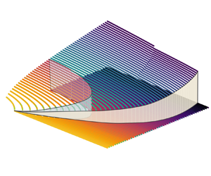
The preceding analysis indicates that the evolution of these hysteresis loops exhibits typical characteristics of a cusp catastrophe (Lopez 1994; Arnold 2003). Our focus now shifts to examining the variations of solutions within the parameter plane of $\lambda$ and $C_{pc}$. Figure 18 provides more states of different cavity pressures and visualises them in a three-dimensional space. The figure showcases the catastrophe surface (Strogatz 2018, chap. 3) in the $\lambda - C_{pc}$ plane, as represented by the amplitudes at the 3/4 chord of the panel. It allows us to know the forms of solutions and their evolutionary trends within the parameter plane. Figure 18(a,b) represent the cases of ascending and descending dynamic pressure, respectively, and figure 18(c) combines the information from panels (a) and (b). The directional arrows in the figure indicate the direction of dynamic pressure change. The red lines beneath the surface illustrate the projection of the critical dynamic pressure onto the $\lambda - C_{pc}$ plane. To provide a more intuitive explanation, a schematic representation of figure 18(a,b) is presented in figure 19, where the red arrows describe the behaviour of the solutions as the dynamic pressure changes.

Figure 18. Amplitudes in the $\lambda - C_{pc}$ plane with (a) $\lambda$ ascending, (b) $\lambda$ descending and (c) the combination of panels (a) and (b).

Figure 19. Schematic representation of the catastrophe surface with (a) $\lambda$ ascending and (b) $\lambda$ descending.

Combining figures 18 and 19, it can be observed that regardless of whether the dynamic pressure is ascending or descending, the system undergoes a sharp and discontinuous transition between the flutter and static deformation states at specific positions where the surface cracks. As the cavity pressure increases, the intensity of this transition gradually attenuates and eventually transforms into a continuous evolution after $C_{pc}>1.227$. The projection of the critical dynamic pressure in figure 18(c) highlights the region between the $\lambda _{cr,ascend}$ and $\lambda _{cr, descend}$, which represents the hysteresis structure. Based on figure 18, the critical dynamic pressures of ascending and descending processes intersect at the boundary between Phase II and Phase III. After entering Phase III, the ascending and descending critical dynamic pressures merge into the same line.

To sum up, the variations in $\lambda$ and $C_{pc}$ lead to the following phenomena.

1. 1. The stability boundaries of the system (i.e. the critical dynamic pressures of ascending and descending processes) intersect and form a cusp.

2. 2. At the cusp, the changes in the system stability transition from discontinuous jumps to continuous smooth evolutions.

These analyses indicate that the disappearance of the hysteresis loop and the formation of the cusp are induced by the variations in cavity pressure. The variations trigger a cusp catastrophe phenomenon (Arnold 2003) in the parameter plane of cavity pressure coefficient and non-dimensional dynamic pressure. Due to the inherent complexity of the dynamical system, providing rigorous theoretical proof for this catastrophe phenomenon is challenging. Following the methodology presented by Liu & Dowell (2004), this study employs meticulous numerical methods to determine the evolution pattern of the dynamical system in the parameter plane. The results demonstrate that the system exhibits the principal characteristics of a cusp catastrophe phenomenon.

Similar cusp catastrophe phenomena have also been observed in various other nonlinear systems (Lopez 1994; Böttcher, Nagler & Herrmann 2017), indicating the existence of perilous explosive branch transitions in the dynamical system (Arnold 2003). As depicted in figure 18, such branch transitions occur between Phase II and Phase III, highlighting a crucial finding: the cavity pressure can modulate the stability characteristics of the system. In contrast to the sharp transitions in Phases I and II, when the cavity pressure falls within Phase III, the dynamical system exhibits a more moderate response and the critical dynamic pressure for flutter is higher. Effectively harnessing this favourable feature might potentially enhance the performance of vehicles in extreme operating conditions.

7. Three types of bifurcation induced by cavity pressure

The fundamental nature of the cusp catastrophe phenomenon triggered by cavity pressure lies in its influence on the critical dynamic pressure and how the system transitions at the critical point. Furthermore, the cavity pressure modifies the locations and types of the bifurcations in the system. To examine the variations in system bifurcations under different cavity pressures, an analysis is conducted on the changes in the critical dynamic pressure, which represents the location of the bifurcation occurrence.

Using the fixed points obtained in § 5.1 and limit cycles obtained in § 6.1, figure 20 illustrates the variations of the critical dynamic pressure in the parameter plane of non-dimensional dynamic pressure and cavity pressure coefficient. The solid lines in three different colours represent the critical dynamic pressures obtained in the ascending and descending processes, which correspond to the projections in figure 18. The square dots are the stability boundary of fixed points obtained in § 5.2, which is in excellent agreement with the position where fixed points disappear and become a limit cycle in the numerical calculations. As depicted in figure 20, the $\lambda _{cr, ascend}$ (i.e. the blue and green lines) and the $\lambda _{cr, descend}$ (i.e. the red line) exhibit a pronounced asymmetric distribution on either side of the mean pressure (i.e. $C_{{pc, mean}} \equiv 1.2$). With an increase in cavity pressure, both the $\lambda _{cr, ascend}$ and $\lambda _{cr, descend}$ initially decrease and then increase. At the boundary between Phase I and Phase II (i.e. $C_{pc}=1.208$), the $\lambda _{cr, ascend}$ begins to appear within the investigated range of dynamic pressure. At the boundary between Phase II and Phase III (i.e. $C_{pc}=1.227$), the critical dynamic pressure lines start merging, forming a cusp.

Figure 20. Critical dynamic pressure in the $\lambda - C_{pc}$ plane.

It is important to note that the critical dynamic pressure in the ascending process (red line) in figure 20 shows a tendency to extend downwards to Phase I at the cavity pressure coefficient of 1.208. This suggests the possibility of a $\lambda _{cr, ascend}$ in the high $\lambda$ range of Phase I. Therefore, after considering a wider range of $\lambda$, a reevaluation of the boundary between Phase I and Phase II becomes necessary, and the situation of the existence of $\lambda _{cr, ascend}$ at various cavity pressures cannot be disregarded. Further computations indicate that when the cavity pressure coefficient is 1.207, the system exhibits a $\lambda _{cr, ascend}$ at $\lambda =2420$, and when the cavity pressure coefficient is 1.206, the $\lambda _{cr, ascend}$ exceeds 5000. In other words, after considering a larger range of $\lambda$, the current extent of Phase I needs to be further narrowed. This implies that previous studies, which only focused on the mean cavity pressure, failed to identify the presence of the $\lambda _{cr, ascend}$. This occurrence is attributed to the fact that the $\lambda _{cr, ascend}$ is concealed by the cavity pressure in an extremely high $\lambda$ region, which extended beyond the scope investigated in those studies.

The evolution of solution patterns before and after bifurcation provides insights into the characteristics of the bifurcation (Strogatz 2018, chap. 8). In figure 20, the critical dynamic pressure line divides the $\lambda - C_{pc}$ plane into three zones. These zones correspond to three combinations of flutter or static solutions resulting from the ascending and descending processes. Bifurcations occur at the boundaries between adjacent zones, and the transitions of solutions on both sides of these boundaries characterise the properties of the bifurcation. Due to the complexity of the studied object, and the absence of precise and analysable theoretical models, it is not possible to definitively determine the exact type of the bifurcations solely through limited numerical observations (or experiments) (Wei & Yabuno 2019). The present study investigates the evolution of the solutions and their phase portraits in detail, but this observational information is still insufficient to be considered ‘complete’. Therefore, the classification of bifurcations is prefixed with ‘quasi’ indicating that based on the observations, it can be concluded that the bifurcation exhibits the principal characteristics of a specific type of bifurcation.

As shown in figure 20, the bifurcations spanning different zones under different cavity pressures are classified into three types based on the evolution of solutions in the phase portraits:

1. Zone A $\leftrightarrow$ Zone C, quasi-supercritical Hopf bifurcation;

2. Zone B $\leftrightarrow$ Zone C, quasi-subcritical Hopf bifurcation;

3. Zone B $\leftrightarrow$ Zone A, quasi-saddle-node bifurcation of cycles.

The three types of bifurcations occur individually or in combination at different cavity pressures. As shown in figure 20, the quasi-supercritical Hopf bifurcation occurs in Phase III, the quasi-subcritical Hopf bifurcation occurs in Phase II and the quasi-saddle-node bifurcation of cycles occurs at the cavity pressures excluding Phase III, partially overlapping with the region where the quasi-subcritical Hopf bifurcation occurs.

7.1. Zone A–Zone C: quasi-supercritical Hopf bifurcation

First, the bifurcations across Zone A and Zone C are analysed, which exclusively take place in Phase I.

Figure 21 shows the phase portraits on both sides of the bifurcation point of Zone A–C, with a chosen cavity pressure coefficient of 1.23. The stable and unstable fixed points are marked by the blue cross and circle respectively, while the limit cycle is represented by a red trajectory. The arrows in the figure indicate the behaviour of the solutions around the fixed point or limit cycle. This figure illustrates the characteristics of the solutions before and after the bifurcation. Before the bifurcation, the solutions converge to the fixed point, whereas after the bifurcation, the fixed point disappears and the system transitions into limit cycle oscillation.

Figure 21. Phase portraits on both sides of the critical point under typical cavity pressure in the bifurcation of Zone A–C: (a) $\lambda < \lambda _{cr}$; (b) $\lambda > \lambda _{cr}$.

Figure 22 shows the evolution of the solutions at the bifurcation of Zone A–C for typical cavity pressures. Several dynamic pressures are chosen in the neighbourhood of the bifurcation point to demonstrate the evolution of the solutions as the system traverses the bifurcation. In figure 22, the distinction between ascending and descending dynamic pressures is still maintained, with the arrows representing the sequence of the evolution. Unlike figure 21, figure 22 focuses more on the changes that occur in the solutions when approaching and departing the bifurcation point. The coordinates chosen in both figures are $q_{2}$, $\dot {q}{_2}$ and $q_{3}$, which correspond to the three components exhibiting larger amplitudes in the solutions. To provide a clearer explanation, the development process of the solutions is omitted here, and only the fixed point or limit cycle in a fully developed system is presented. In figure 22, the solutions obtained during the ascending and descending processes are identical, which confirms the absence of hysteresis behaviour in this cavity pressure range (i.e. Phase III). As discussed in § 6.2, the system exhibits a continuous evolution at this point. Taking the case of descending dynamic pressure depicted in figure 22(b) as an example, as the system traverses the critical dynamic pressure from small to large, the fixed point expands into a limit cycle. Under this cavity pressure, when the dynamic pressure approaches the right-sided limit of the critical dynamic pressure, the system exhibits a sufficiently small limit cycle.

Figure 22. Evolution at the critical point under typical cavity pressure in the bifurcation of Zone A–C with (a) $\lambda$ ascending and (b) $\lambda$ descending.

The potential unstable structure is numerically investigated by stimulations of multiple initial conditions before and after the bifurcation point (Strogatz 2018; Liu & Dowell 2004). With $q_{2}$ and $\dot {q}_{2}$ as the variables and other components as fixed values, figure 23 illustrates the basin of attraction at a cavity pressure coefficient of 1.23. The corresponding phase portraits are marked by the blue cross, blue circle and red trajectory, which have the same meaning as in figure 21. This result indicates that the system before and after the bifurcation of Zone A–C always exhibits a single solution, without any unstable regions.

Figure 23. Basin of attraction at $C_{pc}=1.23$.

The preceding discussion indicates that the bifurcation of Zone A–C exhibits the characteristics of a supercritical Hopf bifurcation (Shukla & Alam 2011). In an idealised case, a rule of thumb for supercritical Hopf bifurcations is that as the system parameter approaches the critical value, the size of the limit cycle gradually increases according to a proportion of $\sqrt {\lambda -\lambda _{cr}}$ (Strogatz 2018, chap. 8). For the high-dimensional complex system studied in this paper, the topology of the limit cycle is highly distorted, and there is no standard measurement for the size of the limit cycle. Here, the size of the limit cycle is defined as $(q_{i})_{max}-(q_{i})_{fixed}$, where $(q_{i})_{max}$ is the maximum value of the $i$th generalised displacement of the limit cycle and $(q_{i})_{fixed}$ is the $i$th generalised displacement of the fixed point at the critical point. Figure 24 shows the variation of the limit cycle size at the bifurcation point for a cavity pressure coefficient of 1.23. It can be observed that the size of the limit cycle measured by $q_{2}$ and $q_{3}$ is in good agreement with the theoretical formula under a certain proportionality factor. This further confirms the assertion that the supercritical of Zone A–C is characterised by supercritical Hopf bifurcation.

Figure 24. Size of limit cycle measured by (a) $q_{2}$ and (b) $q_{3}$ in the bifurcation of Zone A–C.

Figure 25 presents the response and phase portraits of the system at the bifurcation point of Zone A–C, providing the dynamic process of the transition between fixed point and limit cycle shown in figure 22. Figure 25(a,b) depict the cases where $\lambda$ approaches the bifurcation point from different directions. The figure indicates that in this subcritical Hopf bifurcation, the growth or shrinkage of the limit cycle unfolds at an extremely slow pace, to the extent that the trajectories in its phase portrait almost fill the entire interior of the limit cycle. The envelope of the response exhibits a monotonic and smooth curve, devoid of sudden amplification or attenuation of its amplitude. Overall, the flutter generated through this bifurcation manifests in a more subdued manner. At the critical point, a small-amplitude limit cycle gradually emerges, exhibiting a long-period asymptotic instability. However, correspondingly, when the dynamic pressure decreases and the system regains stability, the convergence process of flutter also takes a long time.

Figure 25. Response and its phase portrait at the critical point in the bifurcation of Zone A–C, $C_{pc}=1.23$: (a) starting from the fixed point to reach the bifurcation point with $\lambda$ ascending; (b) starting from the limit cycle to reach the bifurcation point with $\lambda$ descending.

7.2. Zone B–Zone C: quasi-subcritical Hopf bifurcation

The bifurcation crossing Zone B and Zone C occurs at $\lambda _{cr,descend}$ in Phase II (i.e. cavity pressure coefficient of $1.208{-} 1.227$). Figures 26 and 27 present the phase portraits and the evolution of the solution at the bifurcation point for $C_{pc}=1.21$. The meanings of the markers in the figures are similar to those in figures 21 and 22.

Figure 26. Phase portraits on both sides of the critical point under typical cavity pressure in the bifurcation of Zone B–C: (a) $\lambda _{cr, descend} < \lambda < \lambda _{{cr, ascend}}$; (b) $\lambda > \lambda _{cr, ascend}$.

Figure 27. Evolution at the critical point under typical cavity pressure in the bifurcation of Zone B–C.

As shown in figure 26(a), there is a stable limit cycle and a stable fixed point in Zone B, while in figure 26(b), there is only a stable limit cycle in Zone C. Moreover, the transition between Zone B and Zone C can occur through three distinct paths, namely as follows.

1. Path 1: the fixed point in Zone B to the limit cycle in Zone C (i.e. with $\lambda$ ascending, figure 26a to figure 26b).

2. Path 2: the limit cycle in Zone B to the limit cycle in Zone C (i.e. with $\lambda$ ascending, figure 26a to figure 26b).

3. Path 3: the limit cycle in Zone C to the fixed point in Zone B (i.e. with $\lambda$ descending, figure 26b to figure 26a).

In the case of Path 2 and Path 3, the solutions maintain the topological structure of a limit cycle, regardless of whether the dynamic pressure is ascending or descending. Conversely, for Path 1, as the dynamic pressure descends, the fixed point suddenly disappears and is replaced by a single limit cycle.

Figure 27 presents the details of the transitions occurring in Path 1. The direction of the arrows represents the sequence of the evolution as the dynamic pressure descends. As indicated by the dashed arrow in figure 27, the transition from the fixed point to the limit cycle occurs suddenly (Strogatz 2018, chap. 8). In further computations, this jumping phenomenon persists and does not disappear as the intervals of dynamic pressure decrease. Compared with the case where the size of the limit cycle size tends to zero in the quasi-supercritical bifurcations, the size in figure 27 exhibits a non-zero minimum value. As the dynamic pressure descends and crosses the bifurcation point, the original fixed point loses stability and gives rise to a stable limit cycle with a larger amplitude. With further increases in the dynamic pressure, the size of the limit cycle continues to grow.

Figure 28 investigates the influence of initial conditions when the cavity pressure coefficient is 1.21. The meanings of the marks are similar to those in figure 23. The bifurcation of Zone B–C corresponds to the range $\lambda =420 \thicksim 500$ in the figure. The unstable structures appear at the boundary between the black and white points. These unstable structures gradually collapse to the fixed point as $\lambda$ ascends, eventually resulting in the collision and engulfment of the unstable structure with the fixed point. Following the disappearance of unstable structures (i.e. at $\lambda = 500$ in figure 28), the system becomes entirely attracted to the limit cycle.

Figure 28. Basin of attraction at $C_{pc}=1.21$.

The above results indicate that the bifurcation of Zone B–C exhibits characteristics of subcritical Hopf bifurcation (Subramanian, Sujith & Wahi 2013; Pasche, Avellan & Gallaire 2021). Building upon this, this study further analyses the response characteristics of Path 1 during the bifurcation. Figure 29 presents the response and phase portrait of the system at the bifurcation point of Zone B–C, corresponding to the dynamic process of the jump shown in figure 27. Specifically, figure 29 showcases the state with $C_{pc}=1.21$ as a representative, while other bifurcations of Zone B–C exhibit similar characteristics.

Figure 29. Response and its phase portrait at the critical point in the bifurcation of Zone B–C.

Compared with the previous subcritical Hopf bifurcation, the occurrence of flutter behaviour in this subcritical bifurcation is more perilous. First, the time course of the limit cycle growth is shorter. Second, from the perspective of the response envelope, there is an explosive process during the growth of the limit cycle, characterised by a sharp increase in amplitude. This phenomenon is also confirmed by the phase portrait. Compared with figure 25(a), the trajectory distribution of solutions in figure 29 during the transition process from the fixed point to the limit cycle is noticeably sparser, indicating a rapid and pronounced change process.

7.3. Zone B–Zone A: quasi-saddle-node bifurcation of cycles

The bifurcation crossing from Zone B to Zone A occurs in all cavity pressure ranges except Phase III and during the process of decreasing dynamic pressure. Notably, in Phase II, the bifurcations of Zone B to A and Zone B to C coexist, resulting in two critical dynamic pressures. Therefore, in addition to the more general case represented by the state with $C_{pc}=1.19$, figure 30(a,b) specifically select the state with $C_{pc}=1.21$ as a representative of Zone B–A bifurcation in Phase II. As shown in figure 30, there is a single stable fixed point in Zone A, while both a stable fixed point and a stable limit cycle are in Zone B. The transition between Zone A and Zone B can occur through three distinct paths, namely as follows.

1. Path 1: the limit cycle in Zone B to the fixed point in Zone A (i.e. with $\lambda$ descending, figure 30b to figure 30a).

2. Path 2: the fixed point in Zone B to the fixed point in Zone A (i.e. with $\lambda$ descending, figure 30b to figure 30a).

3. Path 3: the fixed point in Zone A to the fixed point in Zone B (i.e. with $\lambda$ ascending, figure 30a to figure 30b).

Figure 30. Phase portraits on both sides of the critical point under typical cavity pressure in the bifurcation of Zone B–A: (a) $\lambda < \lambda _{cr,descend}$; (b) $\lambda _{cr,descend} < \lambda < \lambda _{cr,ascend}$; (c) $\lambda < \lambda _{cr}$; (d) $\lambda > \lambda _{cr}$.

For Path 2 and Path 3, the solutions maintain the topological structure of a fixed point, regardless of whether the dynamic pressure is ascending or descending. Conversely, for Path 1, as the dynamic pressure descends, the limit cycle suddenly disappears and is replaced by a single fixed point. In terms of the topological structure of solutions, the states with $C_{pc}=1.21$ and $C_{pc}=1.19$ exhibit consistent patterns. The presence of Zone B–C bifurcation in Phase II does not introduce any new topological structures in the phase portraits. Among the states considered in this study with cavity pressure coefficients ranging from $1.18$ to $1.227$, all the bifurcations of Zone B–C follow the same qualitative patterns. Therefore, in this case, the analysis of the evolution at the bifurcation point is focused on the states where $C_{pc}=1.21$.

Figure 31 shows the details of the transitions in Path 1. As indicated by the solid arrow in figure 31, as the dynamic pressure approaches the critical value, the limit cycle starts to stack and the size of the limit cycle gradually converges to a non-zero value. After the dynamic pressure crosses the critical value, as shown by the dashed arrows in figure 31, the limit cycle suddenly disappears and the system only has a fixed point solution. This transition from a limit cycle to a fixed point does not disappear as the dynamic pressure interval decreases.

Figure 31. Evolution at the critical point under typical cavity pressure in the bifurcation of Zone B–A.

The influence of initial conditions is also investigated here, and the bifurcation of Zone B–A corresponds to the process of $\lambda =360 \thicksim 420$ shown in figure 28. When $\lambda =380$ and 400, the system exhibits an unstable structure with a complex topology, which evolves from the general case at $\lambda =420$. Furthermore, when $\lambda =360$, the unstable structure completely disappears and the system is entirely attracted by the limit cycle. The same characteristics are also observed in the example of $C_{pc}=1.19$ shown in figure 32, indicating that the development of this unstable structure and its erosion of the attractor region of the limit cycle are common features in such bifurcations of Zone B–A. Regarding the complex case of $\lambda =400$, the unstable structure considering $q_{3}$ is depicted in figure 33. By incorporating the $q_{3}$ dimension, it can be observed that this unstable structure exhibits multi-layered characteristics. This structure possesses a complex high-dimensional topology, and the low-dimensional projection presented here merely represents its local features. However, it is clear that this unstable structure approaches and compresses the attractor region of the limit cycle as the dynamic pressure descends.

Figure 32. Basin of attraction at $C_{pc}=1.19$.

Figure 33. Basin of attraction at $C_{pc}=1.21$, $\lambda = 400$.

The half-stable cycle that burns in the collision is the principal characteristic of the saddle-node bifurcation of cycles (Wei & Yabuno 2019; Zhu et al. 2020). From the neighbourhood of this half-stable cycle, the trajectories of the solutions can be classified into two types: one is attracted to the half-stable cycle itself, while the other is repelled to the fixed point (Holmes 1977). To locate this half-stable cycle, we start from the neighbourhood of the limit cycle solution and observe the trend of the solutions. This action is accomplished by introducing a small perturbation to the system, with each component of the solution being perturbed individually. The perturbation value is set to 1 % of the amplitude of that component, and both positive and negative perturbations are considered. The results indicate that in the bifurcation of Zone B–A, the limit cycle at the critical dynamic pressure attracts only part of the perturbations while repelling others, with the solutions repelled by the limit cycle eventually attracting to the fixed point.

Figure 34 shows several states of the system. At a non-dimensional dynamic pressure of 374.75 (i.e. the critical dynamic pressure for $C_{pc}=1.21$), the limit cycle attracts perturbations in the positive direction of $\dot {q}_{2}$ and repels perturbations in the negative direction. This behaviour indicates that the limit cycle at the critical dynamic pressure exhibits a half-stable state. Furthermore, when $\lambda > \lambda _{\mathrm {cr}}$, the limit cycle attracts all neighbouring trajectories and becomes stable. Conversely, when $\lambda < \lambda _{cr}$, the limit cycle disappears and any perturbations are attracted to the single fixed point. The existence of this half-stable cycle further confirms the characteristics of a saddle-node bifurcation of cycles in the bifurcations of Zone B–A (Strogatz 2018, chap. 8).

Figure 34. Stability of limit cycles under different $\lambda$, $C_{pc}=1.21$.

In the bifurcations of Zone B–A under different cavity pressures, the topological structure of the solutions is similar, but there are certain differences in the system's response characteristics at the bifurcation. Figure 35 presents the response and phase portraits of the system at the bifurcation points for three typical cavity pressures. Here, we focus on the dynamic process of the limit cycle-to-fixed point transition in Path 1, where the system starts from the limit cycle and reaches the bifurcation point with the dynamic pressure descending. Specifically, figure 35(a) corresponds to a state with $C_{pc}=1.21$ in Phase II, figure 35(b) represents a state with $C_{pc}=1.205$ in Phase I, where $C_{pc}$ is greater than $C_{pc,mean}$, and figure 35(c) represents a state with $C_{pc}=1.19$ in Phase I, where $C_{pc}$ is lower than $C_{pc,mean}$.

Figure 35. Response and its phase portrait at the critical point in the bifurcation of Zone B–A for (a) $C_{pc}=1.21$, (b) $C_{pc}=1.205$ and (c) $C_{pc}=1.19$.

Compared with the shrinkage of the limit cycle in supercritical Hopf bifurcation (figure 25b), a common feature in the three cases shown in figure 35 is that the shrinkage of the limit cycle occurs over a shorter period and there is an explosive decrease in the amplitude. However, the difference among these three cases lies in the fact that, as the cavity pressure decreases, the shrinkage of the limit cycle experiences a longer bottleneck (Strogatz 2018, chap. 4).

The characteristics of this bottleneck are also different under different cavity pressures. As shown in figure 35(a), corresponding to Phase II, the amplitude of the limit cycle first undergoes a slight monotonic decrease and then exhibits an explosive reduction.

In figure 35(b), corresponding to Phase I, after reaching the bifurcation point, the amplitude of the limit cycle starts to oscillate rhythmically. The frequency of this rhythmic behaviour gradually decreases over time, while the maximum amplitude increases. The limit cycle remains in this rhythmic behaviour for a considerable period before entering an explosive reduction process. During this bottleneck, the rhythmic behaviour initially shows a diverging tendency but suddenly transitions to a stage of convergence of amplitude.

Upon further examination of figure 35(c), where the cavity pressure is lower than $C_{\mathrm {pc, mean}}$, the bottleneck lasts longer, and the rhythmic behaviour exhibits more intricate details. Figure 35(c) also provides the magnified views of the dashed boxes. In this case, the rhythmic behaviour of the limit cycle is initially less pronounced. However, over an extended period of evolution, this rhythmic behaviour gradually diverges, leading to a significant increase in the limit cycle's amplitude at the end of the bottleneck. Subsequently, an explosive reduction in amplitude occurs.

In general, for this quasi-saddle-node bifurcation of cycles, the disappearance of the limit cycle is rapid, accompanied by a significant explosive reduction in amplitude. The majority of the time during the limit cycle shrinkage process is dedicated to traversing the bottleneck (Strogatz 2018, chap. 4), which increases in length as the cavity pressure decreases. During the bottleneck, the limit cycle exhibits rhythmic behaviour, which can be interpreted as the system's response to the disturbance of ‘the dynamic pressure gradually approaching the bifurcation critical point’. This rhythmic behaviour gradually diverges over time and, once it reaches a certain level of divergence, the system undergoes a rapid convergence in amplitude, marking the end of the limit cycle shrinkage process.

8. Conclusions

In this study, the bifurcation characteristics of a panel subjected to both oblique shock and cavity pressure are investigated using the CFD/CSD and reduced-order model methods. The hysteresis behaviour and catastrophe phenomena resulting from these effects are also analysed. The main conclusions are as follows.

1. (i) The amplitude and critical dynamic pressure of the dynamical system exhibit varying degrees of nonlinear changes under different cavity pressures. This phenomenon introduces additional uncertainty in the calculation of panel flutter in the presence of shock, as even slight changes in cavity pressure can have a significant impact. This finding provides a partial explanation for the dispersion of results observed in the previous studies by Visbal (2012) and Li et al. (2019).

2. (ii) The cavity pressure governs the hysteresis behaviour of the dynamical system. This hysteresis behaviour introduces multi-stability and makes the system highly sensitive to initial conditions. Calculations that employ fixed initial conditions can lead to unpredictable results falling onto either the upper or lower branch of the hysteresis loop. The present study provides supplementary analysis and comparative insights into the jump phenomenon reported by An et al. (2021).

3. (iii) The variation of cavity pressure triggers the cusp catastrophe phenomenon in the cavity pressure coefficient – non-dimensional dynamic pressure plane. As the cavity pressure changes, the transition of the system at the cusp point, where the ascending and descending critical pressures merge, shifts from continuous evolutions to explosive growth. Appropriate cavity pressure allows the system to exhibit long-period asymptotic instability characteristics, effectively preventing the occurrence of dangerous explosive flutter.

4. (iv) The investigated system displays three types of bifurcation phenomena, exhibiting characteristics akin to supercritical Hopf bifurcation, subcritical Hopf bifurcation and saddle-node bifurcation of cycles, respectively. These bifurcations occur individually or in combination under different cavity pressures. This evolution of the bifurcations, driven by changes in cavity pressure, is the root cause of the cusp catastrophe. In the supercritical Hopf bifurcation, the system smoothly enters or exits the flutter state. However, in both subcritical Hopf bifurcation and saddle-node bifurcation of cycles, the transition of the system involves an unavoidable explosive process. Moreover, in the saddle-node bifurcation of cycles, the limit cycle exhibits rhythmic behaviour, and the duration and magnitude of this behaviour increase as the cavity pressure decreases.

This study contributes to a deeper understanding of the nonlinear dynamical behaviour of panels in real complex environments. It provides new explanations for the discrepancies reported in previous research on the aeroelasticity of panels. Additionally, the study highlights the significant potential of cavity pressure in modulating the stability characteristics of the system. Specifically, a specific level of cavity pressure (i.e. Phase III) not only introduces moderate instability characteristics to the system, but also expands the stability boundary. Harnessing this favourable feature could potentially enhance the performance of vehicles in extreme operating conditions. Therefore, future research will focus on exploring methods to use cavity pressure as a means to improve the stability characteristics of the system.