Non-continuum effects on the sound of a heated line source: from a monopole to non-isotropic radiation

Abstract

We study the effect of continuum breakdown on the two-dimensional thermoacoustic radiation of a thin plate set in a perfect monatomic gas. The plate is heated harmonically in time and the acoustic field is investigated in the entire range of gas rarefaction rates. Analytical approximations are obtained in the limits of high (free-molecular) and low (continuum limit) gas rarefaction, accompanied by direct simulation Monte Carlo calculations at intermediate flow conditions. While the source acoustic field is of a monopole type in the continuum regime, it turns non-isotropic at non-continuum conditions, exhibiting dipole directivity and exponential decay rate in the collisionless limit. The combined effects of source heating frequency and gas Knudsen number on the far-field acoustic radiation are illustrated and rationalized.

1. Introduction

Thermoacoustic sound generation by unsteady heating of a structure has been commonly addressed as a canonical problem in continuum acoustics (Howe 1998; Pierce 2019). Serving as a benchmark test case for examining the production and propagation of sound waves in fluids, thermoacoustic sound radiation has been additionally suggested in several applications, including biomedical thermoacoustic imaging (Oraevsky et al. 1994) and heat-driven flow animation (Yariv & Brenner 2004). In an effort to develop efficient means for ultrasonic sound emission, thermoacoustic sound has also been applied in the development of the thermophone (Arnold & Crandall 1917; Wente 1922; Shinoda et al. 1999), which was later considered as a useful apparatus for the cancellation of vibroacoustic noise (Julius et al. 2018; Leizeronok et al. 2023).

The propagation of thermoacoustic sound at non-continuum conditions in gaseous media has been investigated in a sequence of works. These become relevant wherever the characteristic length scale, or time scale, of the set-up involved become of the order of the molecular mean free path, or time, respectively. Focusing on an infinite planar heated surface (see Sone (1965), Wadsworth, Erwin & Muntz (1993), Manela & Hadjiconstantinou (2007, 2010), Nassios, Yap & Sader (2016) and papers cited therein), existing studies have analysed the attenuating effect of gas rarefaction, resulting in decay rates greater than at continuum conditions. Later works have demonstrated that thermoacoustic sound, caused by boundary heat-flux excitations, may be applied to monitor the noise of a vibrating planar object (Manela & Pogorelyuk 2014, 2015). The planar-wall investigations have been followed by works on non-planar (yet unidirectional) source geometries, including cylindrical (Kalempa & Sharipov 2014; Ben Ami & Manela 2017) and spherical (Ben Ami & Manela 2019) body configurations.

Almost invariably, existing investigations on non-continuum thermoacoustic sound radiation have considered one-dimensional problems, where signal propagation was permitted only in the direction normal to the source boundaries. While such an assumption significantly simplifies the analysis, it is evidently desirable to extend the current knowledge and investigate the effect of system two-dimensionality on thermoacoustic sound propagation. Until recently, only a few works have considered two-dimensional sound propagation in rarefied gases, focusing on vibroacoustic set-ups. To this end, Wu (2016) has examined the propagation of acoustic waves in a rarefied gas confined in a two-dimensional cavity, generated by mechanical oscillations of one of the bounding surfaces. In a different work, Yap & Sader (2016) have studied the acoustic field of an oscillating rigid sphere, applying the Bhatnagar–Gross–Krook model of the Boltzmann equation for the analysis. Lately, the two-dimensional sound radiation by a non-uniformly vibrating plane in semi-infinite (Manela & Ben-Ami 2021) and straight channel (Manela & Ben-Ami 2022) configurations has been examined, demonstrating the qualitative impact of continuum breakdown on the vibroacoustic field amplitude and directivity.

In view of the above, the objective of the present contribution is to analyse the effect of gas rarefaction on the two-dimensional acoustic radiation of a time-periodically and uniformly heated body. While it is known that such sources are of a monopole type in the continuum limit (Howe 1998; Pierce 2019), the combined impacts of surface non-isotropicity and deviation from continuum on their thermoacoustic radiation have not been considered hitherto. For geometrical simplicity, we consider the case of a planar finite thin plate. The problem is investigated over the entire range of gas rarefaction rates. Analytical approximations are presented in the limits of high (free-molecular) and low (continuum limit) rarefaction rates, accompanied by direct simulation Monte Carlo  (DSMC) calculations at intermediate conditions.

In the next section, the two-dimensional heated plate problem is stated. The analytical treatments in the free-molecular and near-continuum regimes are described in §§ 3 and 4, respectively, followed by an outline of the numerical DSMC scheme in § 5. Our results are illustrated in § 6, followed by our conclusions in § 7. Technical details are relegated to the appendices.

2. Statement of the problem

Consider a two-dimensional set-up consisting of an infinitely thin stationary plate of length $L^*$ surrounded by an infinite expanse of a perfect monatomic gas of uniform density $\rho _{0}^{*}$ and temperature $T_{0}^{*}$ (hereafter asterisks denote dimensional quantities). The plate is aligned with the $x_1^*$-axis and placed between $-L^*/2\leq x_1^*\leq L^*/2$, whereas the $x_2^*$-axis is perpendicular to the plate in the $(x^*_1,x^*_2)$ plane. The axes’ origin is located at the midchord of the plate. The gas is initially set at rest and in thermodynamic equilibrium with the plate. At time $t^{*}\geq 0$, the plate temperature $T_{w}^{*}$ is uniformly perturbed via

(2.1)\begin{equation} T_{w}^{*}\left(t^{*}\right)=T_0^*[1+\varepsilon T_{per}(t^{*})], \end{equation}

where $T_{per}(t^*)$ is prescribed and $\varepsilon \ll 1$, so that the system description may be linearized about its initial equilibrium. In the following we analyse the effect of gas rarefaction on the propagation of thermoacoustic sound generated by the heated plate. While the analysis is partly carried out for arbitrary small-amplitude actuations (see § 3), our results focus on harmonic wall excitations,

(2.2)\begin{equation} T_{per}^{*}(t^{*})=\sin(\omega^{*}t^{*}), \end{equation}

where $\omega ^*$ denotes the surface heating frequency. We focus on studying the final time-periodic state of the system.

To render the problem dimensionless, we identify the problem characteristic length and velocity scales with the plate length $L^*$ and molecular mean thermal speed $U^{*}_{th}=\sqrt {2\mathcal {R}^*T_0^*}$ (where $\mathcal {R}^*$ marks the specific gas constant), respectively. The non-dimensional problem is then governed by the gas mean Knudsen number and scaled frequency,

(2.3a,b)\begin{equation} {Kn}=l^{*}/L^{*} \quad \mathrm{and} \quad \omega={\omega^{*}L^{*}}/{U_{th}^{*}}, \end{equation}

respectively, where $l^*$ marks the molecular mean free path. Considering a hard-sphere gas $l^*=m^*/(\sqrt {2}{\rm \pi} \rho _0^*d^{*2})$, where $m^*$ and $d^*$ are the molecular mass and diameter, respectively (Kogan 1969). The choice of a hard-sphere gas model of interaction is made due to its relative simplicity for deriving analytical results, and the effect of using a different (Maxwell) type of molecular interaction is illustrated in § 6. Application of more realistic models of interaction, such as the ab initio potential suggested recently by Sharipov in different contexts (Sharipov 2017; Sharipov & Dias 2018), may be carried out, yet would hinder the analysis and is therefore not followed here. In terms of the governing parameters, free molecular conditions are expected to prevail where ${Kn}\gg 1$ or $\omega {Kn}={\omega ^{*}l^{*}}/{U_{th}^{*}}\gg 1$, for which either the length scale or time scale is short compared with the mean free path or mean free time, respectively. Inversely, continuum-limit conditions require that both ${Kn}\ll 1$ and $\omega {Kn}\ll 1$.

The problem in the free-molecular limit is analysed in § 3. Continuum-limit conditions are discussed in § 4, based on continuum acoustics theory. Details on the applied numerical DSMC scheme are given in § 5.

3. Free-molecular limit

Free-molecular conditions should prevail wherever ${Kn}\gg 1$ or $\omega {Kn}\gg 1$, for which either the system length scale or time scale is short compared with the mean free path or mean free time, respectively. For the two-dimensional set-up considered, the gas state is governed by the probability density function $f=f(t,\boldsymbol {x},\boldsymbol {\xi })$ of finding a gas molecule with position and velocity about $\boldsymbol {x}=(x_1,x_2)$ and $\boldsymbol {\xi }=(\xi _1,\xi _2,\xi _3)$, respectively, at time $t$. While the hydrodynamic (macroscopic) gas motion is confined to the $(x_1,x_2)$ plane, molecular gas movements are distributed in all spatial directions. Expanding $f(t,\boldsymbol {x},\boldsymbol {\xi })$ about its nominal non-dimensional Maxwellian distribution $F={\rm \pi} ^{-3/2}\exp [-\xi ^{2}]$, we put

(3.1)\begin{equation} f\left(t,\boldsymbol{x},\boldsymbol{\xi}\right)=F[1+ \varepsilon\phi(t,\boldsymbol{x},\boldsymbol{\xi})], \end{equation}

where $\phi (t,\boldsymbol {x},\boldsymbol {\xi })$ denotes the unknown perturbation function due to plate heating. At free-molecular conditions, $\phi (t,\boldsymbol {x},\boldsymbol {\xi })$ satisfies the collisionless two-dimensional ($\boldsymbol {x}$-dependent) Boltzmann equation (Kogan 1969),

(3.2)\begin{equation} \frac{\partial \phi}{\partial t}+\xi_{1}\frac{\partial \phi}{\partial x_1}+\xi_{2}\frac{\partial \phi}{\partial x_2}=0. \end{equation}

The equation is supplemented by the initial condition

(3.3)\begin{equation} \phi(t=0^{-},\boldsymbol{x},\boldsymbol{\xi})=0,\end{equation}

together with a linearized form of the diffuse boundary condition at the plate's top ($x_2=0^+$) and bottom ($x_2=0^-$) surfaces,

(3.4)\begin{equation} \phi(t,-1/2\leq x_1\leq 1/2,x_2=0^{{\pm}},\boldsymbol{\xi}\boldsymbol{\cdot}\hat{\boldsymbol{x}}_{\boldsymbol{2}}\gtrless0)=\rho_{per}\left(t\right)+(\xi^{2}-3/2)T_{per}\left(t\right), \end{equation}

applied to the reflected $\xi _{2}\gtrless 0$ molecules at $x_2=0^{\pm }$, respectively. Here, $\hat {\boldsymbol {x}}_{\boldsymbol {2}}$ denotes a unit vector in the positive $x_2$-direction and $\rho _{per}(t)$ is treated unknown. The latter is a function of the time only (thus independent of the location along the plate), in line with the uniformity of the heating signal in (2.1) and the problem symmetry between the top and bottom solid surfaces. Yet, the following scheme could also be applied, with some modifications, to cases where non-uniform heating is imposed at the body. The diffuse condition applied in (3.4) may be viewed as a limit case of the Maxwell condition with a unity accommodation coefficient. Focusing on the effect of wall heating on sound transmission, a fully diffuse wall is considered, as the specular part of reflection (appearing for an accommodation coefficient lower than unity) does not communicate the plate disturbance to the gas. Due to problem linearity, the results for any accommodation coefficient lower than unity may easily be obtained through simple manipulation of our data.

The Maxwell fully diffuse model of gas–solid interaction has been chosen due to its simplicity and the ability to derive analytical solutions from it. The condition should be treated as a kinetic means by which the wall-heating signal is transferred to the gas. It is clear that, by using a different wall condition, the gas temperature at the wall would differ from the one imposed by the present model, and the results should be quantitatively affected. This should be the case when imposing, for example, the Cercignani–Lampis boundary interaction kernel, as suggested in recent works by Graur et al. on set-ups containing temperature gradients (Brancher et al. 2021; Johansson et al. 2023). In the following, we prefer model simplicity over a more involved treatment of the boundary interaction, that should only quantitatively affect the results but obviate analysis.

The problem in (3.2)–(3.4) combined with a decay condition at $|\boldsymbol {x}|\rightarrow \infty$ is amenable to the closed-form solution

(3.5)\begin{equation} \phi\left(t,x_1,x_2\gtrless0,\boldsymbol{\xi}\right)=\begin{cases} \rho_{per}\left(t_{r}\right)+T_{per}\left(t_{r}\right)\left(\xi^{2}-3/2\right), & \xi_2\gtrless0 \ \land\ 0\leq x_{1r}\leq 1\\ 0, & \mathrm{otherwise}, \end{cases} \end{equation}

where

(3.6a,b)\begin{equation} t_{r}=t-x_2/\xi_2 \quad \mathrm{and} \quad x_{1r}=x_1-x_2\xi_1/\xi_2 \end{equation}

mark the retarded time and $x_1$-position of the particle at the instant of reflection from the plate boundary. To determine $\rho _{per}(t)$, the macroscopic condition of impermeability,

(3.7)\begin{equation} \int_{-\infty}^{\infty}\xi_2\phi(t,-1/2\leq x_1\leq 1/2,x_2=0^{{\pm}},\boldsymbol{\xi})\, \mathrm{d}\boldsymbol{\xi}=0, \end{equation}

is imposed at the surface, yielding

(3.8)\begin{equation} \rho_{per}\left(t\right)={-}T_{per}\left(t\right)/2. \end{equation}

Substituting (3.8) into (3.5) and then into (3.1), the hydrodynamic perturbations may be computed via velocity-space quadratures over the probability density function (Kogan 1969). In the present linearized regime, these yield in the upper half-plane ($x_2>0$)

(3.9) \begin{align} &\rho\left(t,x_1,x_2>0\right)\nonumber\\ &\quad= {\rm \pi}^{{-}3/2}\int_{-\infty}^{\infty}\phi\mathrm{e}^{-\xi^2}\,\mathrm{d}\boldsymbol{\xi}\nonumber\\ &\quad= \frac{1}{2\sqrt{\rm \pi}}\int_0^\infty T_{per}(t_r)\mathrm{e}^{-\xi^{2}_{2}} \left\{(\xi^{2}_{2}-1)\left[\mathrm{erfc}\left(\frac{x_1-1/2}{x_2}\xi_2\right)- \mathrm{erfc}\left(\frac{x_1+1/2}{x_2}\xi_2\right)\right]\right.\nonumber\\ &\qquad +\frac{\xi_2}{x_2\sqrt{\rm \pi}} \left(\left(x_1-1/2\right)\exp\left[-\left(\frac{x_1-1/2}{x_2}\xi_2\right)^2\right]\right.\nonumber\\ &\qquad \left.\left. -\left(x_1-1/2\right)\exp\left[-\left(\frac{x_1+1/2}{x_2}\xi_2\right)^2\right]\right) \right\}\mathrm{d}\xi_2, \end{align}

(3.10)\begin{align} &u_1\left(t,x_1,x_2>0\right)\nonumber\\ &\quad = {\rm \pi}^{{-}3/2}\int_{-\infty}^{\infty}\xi_1\phi\mathrm{e}^{-\xi^2}\,\mathrm{d}\boldsymbol{\xi} = \frac{1}{2{\rm \pi}}\int_0^\infty T_{per}(t_r)\mathrm{e}^{-\xi_2^2}\nonumber\\ &\qquad \times \left\{\left(\xi_2^2-\frac{1}{2}\right)\left(\exp\left[-\left(\frac{x_1-1/2}{x_2}\xi_2\right)^2\right]-\exp \left[-\left(\frac{x_1+1/2}{x_2}\xi_2\right)^2\right]\right)\right.\nonumber\\ &\qquad +\left(\frac{x_1-1/2}{x_2}\xi_2\right)^2 \exp\left[-\left(\frac{x_1-1/2}{x_2}\xi_2\right)^2\right]\nonumber\\ &\qquad -\left.\left(\frac{x_1+1/2}{x_2}\xi_2\right)^2\exp\left[-\left(\frac{x_1+1/2}{x_2}\xi_2\right)^2\right] \right\}\mathrm{d}\xi_2, \end{align}

(3.11)\begin{align} &u_2\left(t,x_1,x_2>0\right)\nonumber\\ &\quad= {\rm \pi}^{{-}3/2}\int_{-\infty}^{\infty}\xi_2\phi\mathrm{e}^{-\xi^2}\,\mathrm{d}\boldsymbol{\xi}\nonumber\\ &\quad =\frac{1}{2\sqrt{\rm \pi}}\int_0^\infty T_{per}(t_r)\xi_2\mathrm{e}^{-\xi_2^2} \left\{(\xi_2^2-1) \left[\mathrm{erfc}\left(\frac{x_1-1/2}{x_2}\xi_2\right)-\mathrm{erfc}\left(\frac{x_1+1/2}{x_2}\xi_2\right)\right]\right.\nonumber\\ &\qquad + \frac{\xi_2}{x_2\sqrt{\rm \pi}}\left(\left(x_1-1/2\right)\exp\left[-\left(\frac{x_1-1/2}{x_2}\xi_2\right)^2\right]\right.\nonumber\\ &\qquad-\left.\left.\left(x_1-1/2\right)\exp\left[-\left(\frac{x_1+1/2}{x_2}\xi_2\right)^2\right]\right) \right\}\mathrm{d}\xi_2, \end{align}

(3.12)\begin{align} &P_{11}\left(t,x_1,x_2>0\right)\nonumber\\ &\quad = {\rm \pi}^{{-}3/2}\int_{-\infty}^{\infty}\xi_1^2\phi\mathrm{e}^{-\xi^2}\,\mathrm{d}\boldsymbol{\xi}\nonumber\\ &\quad = \frac{1}{2{\rm \pi}}\int_0^\infty T_{per}(t_r)\mathrm{e}^{-\xi_2^2} \left\{\xi_2^3\frac{x_1-1/2}{x_2}\left[1+\left(\frac{x_1-1/2}{x_2}\right)^2\right] \exp\left[-\left(\frac{x_1-1/2}{x_2}\xi_2\right)^2\right]\right.\nonumber\\ &\qquad \left. -\xi_2^3\frac{x_1+1/2}{x_2}\left[1+\left(\frac{x_1+1/2}{x_2}\right)^2\right] \exp\left[-\left(\frac{x_1+1/2}{x_2}\xi_2\right)^2\right]\right.\nonumber\\ &\qquad +\left. \frac{\sqrt{\rm \pi}}{2}\xi_2^2 \left[\mathrm{erfc}\left(\frac{x_1-1/2}{x_2}\xi_2\right)-\mathrm{erfc}\left(\frac{x_1+1/2}{x_2}\xi_2\right)\right] \right\}\mathrm{d}\xi_2, \end{align}

(3.13)\begin{align} &P_{22}\left(t,x_1,x_2>0\right)\nonumber\\ &\quad = {\rm \pi}^{{-}3/2}\int_{-\infty}^{\infty}\xi_2^2\phi\mathrm{e}^{-\xi^2}\,\mathrm{d}\boldsymbol{\xi}\nonumber\\ &\quad = \frac{1}{2\sqrt{\rm \pi}}\int_0^\infty T_{per}(t_r)\xi_2^2\mathrm{e}^{-\xi_2^2} \left\{(\xi_2^2-1) \left[\mathrm{erfc}\left(\frac{x_1-1/2}{x_2}\xi_2\right)-\mathrm{erfc}\left(\frac{x_1+1/2}{x_2}\xi_2\right)\right]\right.\nonumber\\ &\qquad + \frac{\xi_2}{x_2\sqrt{\rm \pi}} \left(\left(x_1-1/2\right)\exp\left[-\left(\frac{x_1-1/2}{x_2}\xi_2\right)^2\right]\right.\nonumber\\ &\qquad \left.\left.- \left(x_1-1/2\right)\exp\left[-\left(\frac{x_1+1/2}{x_2}\xi_2\right)^2\right]\right) \right\}\mathrm{d}\xi_2 \end{align}

and

(3.14)\begin{align} &P_{33}\left(t,x_1,x_2>0\right)\nonumber\\ &\quad = {\rm \pi}^{{-}3/2}\int_{-\infty}^{\infty}\xi_3^2\phi\mathrm{e}^{-\xi^2}\,\mathrm{d}\boldsymbol{\xi}\nonumber\\ &\quad= \frac{1}{4\sqrt{\rm \pi}}\int_0^\infty T_{per}(t_r)\mathrm{e}^{-\xi_2^2} \left\{\xi_2^2\left[\mathrm{erfc}\left(\frac{x_1-1/2}{x_2}\xi_2\right)-\mathrm{erfc}\left(\frac{x_1+1/2}{x_2}\xi_2\right)\right]\right.\nonumber\\ &\qquad +\frac{x_1-1/2}{2x_2}\xi_2 \exp\left[-\left(\frac{x_1-1/2}{x_2}\xi_2\right)^2\right]\nonumber\\ &\qquad \left.- \frac{x_1+1/2}{2x_2}\xi_2\exp\left[-\left(\frac{x_1+1/2}{x_2}\xi_2\right)^2\right] \right\}\mathrm{d}\xi_2, \end{align}

for the density perturbation, $x_1$-velocity, $x_2$-velocity and normal stress deviation components ($P_{11},P_{22}$ and $P_{33}$), respectively. In (3.9)–(3.14), $\mathrm {erfc}(s)=(2/\sqrt {{\rm \pi} })\int _s^\infty \mathrm {e}^{-s^2}\,\mathrm {d}s$ denotes the complementary error function. The counterpart expressions in the lower half-plane ($x_2<0$) follow by symmetry. The acoustic pressure and temperature deviation from equilibrium are given by

(3.15a,b)\begin{align} p\left(t,\boldsymbol{x}\right)=\tfrac{2}{3}\left[P_{11}\left(t,\boldsymbol{x}\right)+P_{22}\left(t,\boldsymbol{x}\right)+P_{33}\left(t,\boldsymbol{x}\right)\right] \quad \mathrm{and} \quad T\left(t,\boldsymbol{x}\right)=p\left(t,\boldsymbol{x}\right)-\rho\left(t,\boldsymbol{x}\right). \end{align}

For later reference it is noted that all hydrodynamic perturbations vanish along the lines of symmetry $x_1\gtrless \pm 1/2$ with $x_2=0$, as no gas particles may be emitted from the wall along its planar direction in the collisionless limit. This observation is, in fact, the very reason for the qualitative difference between the acoustic field directivities in the free-molecular and continuum limits, to be discussed later on (see § 6).

Different from the analysis in the continuum limit (see § 4), the solution in the free-molecular regime, involving the numerical evaluation of the quadratures in (3.9)–(3.14), is valid for arbitrary small-amplitude $T_{per}(t)$ input signals. Focusing on the case of harmonic excitations specified in (2.2), explicit far-field approximations for the hydrodynamic fields may be obtained for $x_2\gg 1$ with $\omega x_2\gg 1$ (i.e. with $\omega \gg x_2^{-1}$) while keeping $x_1\sim O(1)$. The approximation, presented in Appendix A, applies the method of steepest descent (Abramowitz 1953) to evaluate the $\xi _2$-integrals. This yields, for the far-field acoustic pressure

(3.16)\begin{align} & p\left(t,x_1\sim O(1),x_2\gg1;\omega x_2\gg1\right)\nonumber\\ &\quad \approx \frac{\mathrm{i}\omega}{2\sqrt{3{\rm \pi}}}\exp\left[{\rm i}\omega t-z\right] \left[\left(\frac{\mathrm{i}\omega x_2}{2}\right)^{2/3}+\frac{53}{36}+O(x_2^{{-}2/3})\right], \end{align}

where

(3.17)\begin{equation} z=3\left(\frac{\mathrm{i}\omega x_2}{2}\right)^{2/3}=\frac{3}{2}\left(\frac{\omega x_2}{2}\right)^{2/3}\left[1+\mathrm{i}\sqrt{3}\right] . \end{equation}

The above evaluation should be valid at distances $x_2\gg 1$ from the heated plate where $\omega x_2\gg 1$. Since the signal at free-molecular conditions vanishes at short distances from the source, this requires that the actuation frequency is not small. Comparison between our asymptotic and full numerical solutions indicates that the present estimate holds already at $\omega x_2\gtrsim 3$. At the level of approximation presented in (3.16), the far acoustic pressure is independent of $x_1$, as long as $x_1\sim O(1)$, i.e. the observer is located in the relative proximity to the $x_2$-axis.

4. Continuum-limit conditions

Complete analysis of the continuum-limit problem in the present two-dimensional time-periodic set-up requires numerical computation of the entire flow field. To avoid application of heavy-load numerical solvers and gain analytical insight, we focus on the investigation of the system acoustic far-field, contributed by the net rate of heat flux radiated by the plate source to the gas. In the common framework of acoustic analogies, we make use of the dimensional expression for the far-field pressure generated by a heated body (Howe 1998),

(4.1)\begin{equation} p^*(t^*,\boldsymbol{\bar{x}}^*)\approx{-}\frac{1}{c_p^*T_0^*}\frac{\partial}{\partial t^*}\oint_{s^*} q_n^*(\tau,\boldsymbol{\bar{y}}^*)G^*(t^*-\tau^*,\boldsymbol{\bar{x}}^*,\boldsymbol{\bar{y}}^*)\,\mathrm{d}^3\boldsymbol{\bar{y}}^*\,\mathrm{d}\tau^*, \end{equation}

valid at distances $|\boldsymbol {\bar {x}}^*|=(x_1^{*2}+x_2^{*2}+x_3^{*2})^{1/2}\gg L^*$ from a three-dimensional source placed in a fluid at rest. Here, $\boldsymbol {\bar {x}}^*=(x^*_1,x^*_2,x^*_3)$ is the three-dimensional space vector, $c_p^*$ is the gas specific heat capacity at a constant pressure and $s^*$ marks the external surface of the body interacting with the gas. In addition, $q_n^*$ is the time- and position-varying normal heat-flux along the source surface and $G^*$ is the Green's function satisfying the counterpart acoustic problem of a point source placed in the proximity of the body. The scalar $\tau$ and three-dimensional vector $\boldsymbol {\bar {y}}^*=(y_1^*,y_2^*,y_3^*)$ denote the source coordinates of time and space, respectively. We consider an acoustically compact configuration, where the source size $L^*$ is small compared with the radiated acoustic wavelength $\lambda ^*$, namely

(4.2)\begin{equation} \frac{L^*}{\lambda^*}=\frac{\omega^*L^*}{2{\rm \pi} c_0^*}\ll1. \end{equation}

Here, $c_0^*=(\gamma \mathcal {R}^*T_0^*)^{1/2}$ denotes the continuum-limit mean speed of sound in the gas and $\gamma$ is the ratio of specific heats. For the monatomic hard-sphere gas considered hereafter, $\gamma =5/3$. In terms of the scaling introduced in § 2, the compact-body assumption is equivalent to considering the non-large non-dimensional frequencies

(4.3)\begin{equation} \omega\ll{\rm \pi}\sqrt{2\gamma}\approx5.74. \end{equation}

This is in line with the continuum-limit conditions, requiring that $\omega {Kn}\ll 1$, given that ${Kn}\ll 1$. For an acoustically compact system (Howe 1998),

(4.4)\begin{equation} G^*(t^*-\tau^*,\boldsymbol{\bar{x}}^*,\boldsymbol{\bar{y}}^*)=\frac{1}{4{\rm \pi}|\boldsymbol{\bar{X}}^*-\boldsymbol{\bar{Y}}^*|}\delta\left(t^*-\tau^*-\frac{|\boldsymbol{\bar{X}}^*-\boldsymbol{\bar{Y}}^*|}{c_0^*}\right), \end{equation}

where $\delta ({\cdot })$ denotes the Dirac delta function. Additionally, $\boldsymbol {\bar {X}}^*(\boldsymbol {\bar {x}}^*)$ and $\boldsymbol {\bar {Y}}^*(\,\boldsymbol {\bar {y}}^*)$ mark the Kirchhoff vectors for the considered set-up, in which each $j$ component is equal to the incompressible velocity potential of the flow past the plate with a unit speed in the $j$ direction at large distances from the object (Howe 2003). In the current problem, it is sufficient to approximate

(4.5a,b)\begin{equation} \boldsymbol{\bar{X}}^*(\boldsymbol{\bar{x}}^*)\approx\boldsymbol{\bar{x}}^* \quad \mathrm{and} \quad \boldsymbol{\bar{Y}}^*(\,\boldsymbol{\bar{y}}^*)\approx\boldsymbol{\bar{y}}^*, \end{equation}

equivalent to the flow potential of free-space unity flow in each direction, to obtain the leading-order far-field system behaviour. In what follows we apply (4.1) together with (4.4) and (4.5a,b) for the estimation of the present two-dimensional far acoustic field.

To start with, we carry the $y_3^*$-integration over $(-\infty,\infty )$ in (4.1). Since $q_n^*(\tau,\boldsymbol {y}^*)$ is independent of $y_3^*$, it remains to evaluate the $y_3^*$-quadrature over $G^*$, as detailed in Appendix B. This yields

(4.6)\begin{align} \int_{-\infty}^{\infty}G^*(t^*-\tau^*,\boldsymbol{\bar{x}}^*,\boldsymbol{\bar{y}}^*)\,\mathrm{d}y_3^*\approx \frac{\sqrt{c_0^*}}{2{\rm \pi}\sqrt{2|\boldsymbol{x}^*|}}\frac{{H}(t^*-\tau^*-|\boldsymbol{x}^*|/c_0^*)}{\sqrt{ t^*-\tau^*-|\boldsymbol{x}^*|/c_0^*}}=G_{2{D}}^*(t^*-\tau^*,\boldsymbol{x}^*), \end{align}

where ${H}({\cdot })$ denotes the Heaviside function. We substitute (4.6) together with the continuum-based Fourier law,

(4.7)\begin{equation} q_n^*={-}k_0^*\frac{\partial T^*}{\partial y_n^*}, \end{equation}

into (4.1), where $k_0^*$ denotes the coefficient of gas thermal conductivity at equilibrium conditions. Applying the problem symmetry for carrying the $y_2^*$-quadrature along the thin plate surface, we obtain

(4.8)\begin{equation} p^*(t^*,\boldsymbol{x}^*)\approx \frac{k_0^*\sqrt{c_0^*}}{{\rm \pi} c_p^*T_0^*\sqrt{2|\boldsymbol{x}^*|}}\frac{\partial}{\partial t^*} \int_{0}^{[t^*]}\int_{{-}L^*/2}^{L^*/2}\left(\frac{\partial T^*}{\partial y_2^*}\right)_{y_2^*=0^+} \frac{\mathrm{d}y^*_1\,\mathrm{d}\tau^*}{\sqrt{[t]^*-\tau^*}}, \end{equation}

where $[ t^*]=t^*-|\boldsymbol {x}^*|/c_0^*$ marks the dimensional acoustic retarded time. Adopting the scaling in § 2, we arrive at the non-dimensional expression

(4.9)\begin{equation} p(t,\boldsymbol{x})\approx \frac{(2\gamma)^{1/4}}{\rm \pi} \frac{\mu_0\,{Kn}}{Pr}\frac{1}{\sqrt{|\boldsymbol{x}|}} \frac{\partial}{\partial t}\int_{0}^{[t]}\int_{{-}1/2}^{1/2}\left(\frac{\partial T}{\partial y_2}\right)_{y_2=0^+} \frac{\mathrm{d}y_1\,\mathrm{d}\tau}{\sqrt{[t]-\tau}}, \end{equation}

where $[ t]=t-|\boldsymbol {x}|\sqrt {2/\gamma }$. In (4.9), ${Pr}$ and $\mu _0$ denote the Prandtl number and scaled viscosity,

(4.10a,b)\begin{equation} {Pr}=\frac{k_0^*}{\mu_0^*c_p^*} \quad \mathrm{and} \quad \mu_0=\frac{\mu_0^*}{\rho_0^*U_{th}^*l^*}, \end{equation}

respectively, where $\mu _0^*$ marks the dimensional mean dynamic viscosity. For the currently considered monatomic hard-sphere gas, ${Pr}=2/3$ and $\mu _0=5\sqrt {{\rm \pi} }/16$ (Kogan 1969).

Inspecting (4.9), it is observed that the leading-order far acoustic field is of a monopole type, propagating isotropically in all directions. This is qualitatively different from the acoustic directivity at free-molecular conditions, studied in § 3, where sound propagates primarily around the $x_2$-axis normal to the plate, and no signal is detected along the $x_1$-axis (see (3.15a,b) et seq.). As typical to continuum two-dimensional set-ups, the far-field pressure decays with the inverse square root of the distance from the source, $|\boldsymbol {x}|^{-1/2}$, which retains a finite far-field acoustic power (Howe 1998). In the inviscid ${Kn}\rightarrow 0$ limit, the monopole acoustic far-field vanishes, as heat (and subsequent pressure fluctuations) cannot be communicated to the fluid in the absence of gas thermal conductivity.

To proceed with the evaluation of (4.9), the temperature gradient ${\partial T}/{\partial y_2}$ at the plate surface ($y_1\in [-1/2,1/2],y_2=0^{\pm }$) should be determined. While this requires a numerical computation of the near flow field, it is reasonable to assume that when the acoustic wavelength ($=2{\rm \pi} c_0^*/\omega ^*$) is much larger than the heat diffusion scale ($=({k^*_0/(\rho _0^*c_p^*\omega ^*)})^{1/2}$), a condition satisfied by the current acoustically compact and low ${Kn}$ set-up (see (4.2) et seq.), the precise behaviour of the normal temperature gradient near the plate end points is unimportant. Thus, it is appropriate to assume to a leading order that ${\partial T}/{\partial y_2}$ is uniform along the surface and the same as for an infinite plate. Following previous one-dimensional continuum-limit analyses of the thermoacoustic disturbance generated by a time-periodic heated infinite wall (e.g. Manela & Hadjiconstantinou 2010; Leizeronok et al. 2023), the temperature field has been computed and is tabulated in Appendix C for completeness. The temperature gradient at the wall surface $s$ at time $\tau$ is subsequently given by

(4.11)\begin{equation} \left(\frac{\partial T}{\partial y_2}\right)_{(\tau,s)} = \left(D_1r_1+D_2r_2\right)\mathrm{e}^{\mathrm{i}\omega\tau}, \end{equation}

where $r_{1,2}(\omega,{Kn})$ are given by (C7a–c) and $D_{1,2}(\omega,{Kn})$ are specified in (C9a,b). Substituting (4.11) into (4.9), the long-time ($[t]\gg 1$) $\tau$-integral may be evaluated as

(4.12)\begin{equation} \int_0^{[t]}\frac{\exp({\mathrm{i}\omega\tau})}{\sqrt{[t]-\tau}}\,\mathrm{d}\tau=\sqrt{\frac{\rm \pi}{\omega}} \exp({\mathrm{i}\left(\omega[t]-{\rm \pi}/4\right)}), \end{equation}

and the approximate expression for the far-field pressure is given by

(4.13)\begin{equation} p(t,\boldsymbol{x})\approx \frac{(2\gamma)^{1/4}\mu_0\,{Kn}\sqrt{\omega}\left(D_1r_1+D_2r_2\right)}{{Pr\sqrt{{\rm \pi}|\boldsymbol{x}|}}} \exp({\mathrm{i}\left(\omega[t]+{\rm \pi}/4\right)}). \end{equation}

As in (4.9), the far-field pressure decays with the inverse square root of the distance from the origin and vanishes in the inviscid ${Kn}\rightarrow 0$ limit. In line with the imposed heating periodicity and problem linearity, the signal is $\omega$-harmonic. The Knudsen and frequency dependencies of the pressure amplitude (included in both the ${Kn}\sqrt {\omega }$ term and in $D_{1,2}(\omega,{Kn})$ and $r_{1,2}(\omega,{Kn})$ appearing in (4.13)) will be discussed in § 6.

5. Numerical scheme: DSMC method

The DSMC method is widely regarded as the most effective approach for the numerical analysis of rarefied gas flows (Bird 1994). Originally developed as a direct numerical modelling of dilute gas dynamics (Bird 1963), DSMC was later shown to yield results that converge to the solution of the Boltzmann equation in an appropriate limit (Wagner 1992). Within the DSMC framework, the velocity distribution function of the gas molecules is represented by computational particles. The computational domain is divided into cells with sizes smaller than the molecular mean free path $l^*$. Particle motions and interactions are decoupled over a time step shorter than the local mean free time between collisions. At each time step, the particles are first translated as if they do not interact with each other. They are then sorted into cells and collisions are performed stochastically, preserving the collision momentum and energy invariants. Finally, the macroscopic fields in each cell are evaluated by taking weighted averages of the particle properties.

The present work applied the DSMC scheme to simulate the hard-sphere gas response over a wide range of gas rarefaction rates, varying between early transition to free-molecular conditions. A two-dimensional rectangular simulation box was considered, taken large enough to mitigate the spurious reflections resulting from the artificial ‘top’ and ‘side’ bounding walls. Based on the free-molecular analysis in § 3, the acoustic field at ballistic flow conditions vanishes at few plate length scales away from the source. As this distance increases with decreasing rarefaction, numerical experiments have indicated that setting the simulation box size to $15L^*\times 15L^*$ was sufficient to capture the unbounded flow behaviour for ${Kn}\gtrsim 0.1$ and $\omega {Kn}\gtrsim 0.1$. The simulation box was divided into cells of equal size, with dimensions in the range $\Delta s^* = [0.005,0.025]l^*$. The time step was taken as $\Delta t^* = \Delta s^* /(5\sqrt {\mathcal {R}^*T_0^*})$.

Each simulation started with a gas in equilibrium surrounding the plate. At each time step, computational particles were inserted from the outer boundaries of the simulation box, randomly sampled from the equilibrium Maxwellian distribution. Particles crossing the boundaries from the inside of the domain were removed. In line with problem formulation, scattering at the plate surface followed fully diffuse reflections, with the prescribed boundary temperature varying harmonically in time. The simulations were run for $\approx 200$ periods, where the results during each period were recorded at specific times. Once a final periodic state has been reached (typically after $\approx 20$ periods), the results were averaged between remaining periods. A value of $\varepsilon =0.15$ for the heating amplitude (see (2.1)) has proved sufficiently small to neglect nonlinear effects. A typical simulation on a single-processor Intel CoreTM i7-8700 machine (12M cache, up to 4.60 GHz) using the above computational parameters lasted up to a week.

Notably, the application of the DSMC scheme in the present problem faces a significant challenge due to the combination of the weak signal induced by the source and set-up two-dimensionality. These lead to an inevitable non-large signal-to-statistical-noise ratio, hindering the capturing of the low-Mach flow field involved (Hadjiconstantinou et al. 2003). Possible remedies may have included the usage of low-variance DSMC schemes (Homolle & Hadjiconstantinou 2007), weighted particles or deterministic methods such as discrete velocity techniques (Aristov 2001; Ghiroldi & Gibelli 2014). However, these alternatives are less accessible to implement than standard DSMC and are not in the focus of the present contribution. In applying the DSMC method, we have maintained the signal-to-noise ratio sufficiently large by increasing the average number of computational particles per cell to $\approx 1200$. Additionally, the statistical noise was reduced by enforcing the problem symmetry, allowing for the averaging of the simulation results between the domain four quadrants.

6. Results and discussion

Figure 1 presents the free-molecular solution derived in § 3, focusing on the case of $\omega =1$. Figure 1(a) shows a two-dimensional pressure amplitude colourmap, where the plate location is marked by the black solid line. In line with the exponential decay found in (3.16), the acoustic field is confined to only a few length scales away from the plate, and sound is radiated mainly in the direction normal to the surface. The analytical results are compared with DSMC predictions at ${Kn}=10$ in figure 1(b). In support of the closed-form solution, pressure time snapshots at quarter-period ($t=T/4=(2{\rm \pi} \omega )^{-1}$) along $x_1=0$ and $x_2=0.02$ are found in close agreement with DSMC data. Figure 1(b) further illustrates the non-isotropic character of sound radiation at high rarefaction rates, where the sound along $x_2=0.02$ is restricted to the $-0.5\leq x_1\leq 0.5$ interval above the plate, in marked difference from the midchord $x_1=0$ signal, which spreads over a much wider $x_2$-interval.

Figure 1. The free-molecular (${Kn}\rightarrow \infty$) acoustic field at $\omega =1$: (a) pressure amplitude colourmap; (b) quarter-period ($t=T/4$) time snapshots of the $x_2$-variation of the acoustic pressure along $x_1=0$ (black line) and $x_1$-variation along $x_2=0.02$ (blue curve), compared with respective DSMC results at ${Kn}=10$ (symbols); (c) far-field pressure amplitude directivity map, $|p|/|p_{max}|$, at collisionless (blue line) and continuum (black curve) conditions, compared with the directivity of a dipole ($|p|/|p_{max}|=\sin \theta$, dashed black line); (d) velocity amplitude colourmap and streamlines at quarter-period time, $t=T/4$. The black lines in figures 1(a) and 1(d) mark the plate location.

Figure 1(c) shows the far-field pressure amplitude directivity, $|p|/|p_{max}|$, computed at a fixed distance $|\boldsymbol {x}|\gg 1$ from the origin and varying direction. The figure compares between the free-molecular (blue line) and monopole continuum-limit (black circle) results, manifesting the qualitative effect of continuum breakdown on radiation directivity. Markedly, the free-molecular curve is found identical with the directivity of a dipole source at continuum conditions (Howe 1998; Pierce 2019), $|p|/|p_{max}|=\sin \theta$, as denoted by the dashed black line. The present free-molecular field may nevertheless not be referred to as a dipole, as it does not obey to the continuum wave equation and exhibits an exponential decay rate that is far stronger than its continuum counterpart. In practice, in the continuum limit problem, a dipole-type field would have occurred if the upper and lower surfaces of the plate were heated at opposite phases. Our present discussion is limited to the case of uniform excitation only. As stated after (3.16), the far-field free-molecular estimate for the acoustic pressure, strictly valid at distances $x_2\gg 1$ from the source (with $\omega x_2\gg 1$), coincides with the exact ballistic result already at $x_2\approx 3$ for $\omega =1$. Specifically, the ballistic-field directivity presented in figure 1(c) for $\omega =1$ is based on the calculation of the full free-molecular solution at $|\boldsymbol {x}|=4$. At such distances, the continuum-limit monopole directivity of the acoustic pressure is similarly effective (see figure 3f), and the comparison presented between the two ‘far fields’ is in place.

Figure 1(d) presents the instantaneous flow field generated by the source at quarter-period, showing a colourmap of the velocity amplitude and a sequence of streamlines originating in the vicinity of the plate surface. Low speed flow is generated by the thermoacoustic source, reaching a maximum of $|\boldsymbol {u}|\approx 0.047$ at approximately one length scale away at each side of the plate. In accordance with the non-isotropic pressure field, no flow is observed along the $x_2=0$ section. The streamlines that originate close to the plate follow straight lines that reach a stagnation at $|\boldsymbol {x}|\approx {\rm \pi}$, half a wavelength away from the plate midchord, which is a node location at the presented time.

The breakdown of the free-molecular description is examined in figures 2 and 3. To this end, figure 2 compares the $\omega =1$ collisionless acoustic pressure at quarter-period along $x_2=0.02$ (identical to the solid blue line in figure 1b) with the counterpart DSMC predictions at decreasing values of ${Kn}$. At the largest ${Kn}=10$ shown, the DSMC-calculated signal matches well with the free-molecular result. Yet, this agreement breaks down with descending ${Kn}$, where the DSMC-computed pressure is no longer confined to the $-0.5\leq x_1\leq 0.5$ interval above the body, but extends to a larger distance in the platewise direction. This marks the transition from the ballistic non-isotropic to the continuum-limit monopole-type field, enabled by the mechanism of molecular collisions.

Figure 2. Breakdown of the free-molecular description: $x_1$-variations of the acoustic pressure at quarter-period time ($t=T/4$) along $x_2=0.02$ for $\omega =1$ and the indicated values of ${Kn}$. The solid line marks the analytical free-molecular solution (${Kn}\rightarrow \infty$) and the crosses, blue circles and red triangles present DSMC data at the indicated values of ${Kn}=10,2$ and $0.5$, respectively.

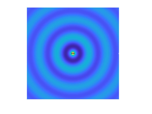
Figure 3. Effect of gas rarefaction on the acoustic pressure at quarter-period time, $t=T/4$: pressure perturbation colourmaps for $\omega =1$ and (a) ${Kn}\rightarrow \infty$, (b) ${Kn}=10$, (c) ${Kn}=2$, (d) ${Kn}=0.5$, (e) ${Kn}=0.2$ and ( f) ${Kn}=0.1$. The black lines in each figure mark the plate location.

A two-dimensional illustration of the conversion between the ballistic and continuum limit regimes is presented in figure 3, where acoustic pressure colourmaps at quarter-period for $\omega =1$ are shown at various Knudsen numbers. While the collisionless (figure 3a) and ${Kn}=10$ (figure 3b) fields appear identical, some deviations from the ballistic result may be observed in figure 3(c) for ${Kn}=2$, where a slight ‘monopole ring’ (marked by the dark blue zone at an $|\boldsymbol {x}|\approx {\rm \pi}$ distance from the origin) is seen. This trend intensifies with decreasing rarefaction, as depicted by figure 3(d–f). Showing a larger portion of the $(x_1,x_2)$ flow plane for better visualization, the formation of a far monopole field is clearly manifested, and becomes most coherent at the lowest ${Kn}=0.1$ presented in figure 3( f).

Figure 4 examines the continuum-limit solution discussed in § 4. Maintaining $\omega =1$, figure 4(a) shows a colourmap of the monopole acoustic pressure for ${Kn}=0.1$ at quarter-period, based on (4.13). The relatively large value of ${Kn}$ (for a continuum-limit solution) was chosen equal to the smallest value of ${Kn}$ simulated (cf. figure 3f), since DSMC calculations at lower Knudsen numbers were too excessive to follow. Remarkably, the quantitative comparison in figure 4(b) of the $x_1=0$ section results between the two methods shows a plausible agreement, supporting the continuum-limit analysis. While the deviations between the schemes' predictions may be associated with the relatively large value of the Knudsen number considered, the general trends of signal decay rate ($\propto |\boldsymbol {x}|^{-1/2}|$) and wavelength (${\sim }2{\rm \pi} /\omega$) appear in satisfactory agreement. The figure also presents the corresponding analytical result in the case of Maxwell molecules, affecting the values of $\mu _0$ and the temperature jump coefficient $\zeta$ in the solution (Sone 2007). The comparison between the dashed blue and solid black curves indicates that the effect of the model of molecular interaction is only quantitative, and the general trends of signal decay rate and wavelength are not affected. To inspect the solution at lower rarefaction rates, figure 4(c) shows the frequency variations of the far-field scaled pressure amplitude, $|\boldsymbol {x}|^{1/2}||p|$, according to (4.13), at the indicated values of ${Kn}$. The continuum-limit scaled amplitude reduces monotonically with both $\omega$ and ${Kn}$. The decrease with $\omega$ reflects the increase in period time and the vanishing of the excitation signal as $\omega \rightarrow 0$ (see (2.2)). The decline with ${Kn}$ occurs since compact body monopole sound may not be emitted in the absence of gas heat conduction (see (4.13) et seq.). The results in figure 4(c) should strictly hold for $\omega \ll 5.74$, in accordance with the compact body assumption made in § 4 (see (4.3)), yet may be qualitatively effective also at somewhat higher frequencies (Howe 1998).

Figure 4. The acoustic pressure in the continuum-limit (${Kn}\ll 1$): (a) colourmap of the acoustic pressure for $\omega =1$ and ${Kn}=0.1$ at time $t=T/4$ based on (4.13); (b) comparison of $x_2$ pressure variations along $x_1=0$ between the analytical ((4.13), black solid line) and DSMC (crosses) results for $\omega =1$ and ${Kn}=0.1$ at time $t=T/4$; (c) frequency variations of the far-field scaled pressure amplitude, $|\boldsymbol {x}|^{1/2}||p|$, according to (4.13), at the indicated values of ${Kn}$. The black line in figure 3(a) marks the plate location. The dashed blue curve in figure 4(b) shows the analytical result for the case of Maxwell molecules.

Finally, the impact of the source heating frequency on the acoustic field is examined in figure 5. Considering a relatively low value of ${Kn}=0.1$, the figure presents acoustic pressure colourmaps at period time, $t=T=2{\rm \pi} /\omega$, at increasing values of $\omega$. Recalling the discussion in § 2 (see (2.3a,b) et seq.), the gas flow regime is determined, apart from the Knudsen number, by the ratio between the surface heating frequency and the frequency of molecular collisions, being $\sim O(\omega {Kn})$. Deviations from continuum conditions may therefore occur even at small values of ${Kn}$, given that $\omega \gtrsim {Kn}^{-1}$. Indeed, the vanishing of the monopole rings between figure 5(a) (for $\omega =1$) and 5(b) (for $\omega =2$), together with the shortening of the acoustic wavenumber, are clearly seen. At $\omega =5$ (figure 5c, where $\omega {Kn}=0.5$) and $\omega =10$ (figure 5d, for which $\omega {Kn}=1$), the acoustic perturbations are confined to the very proximity of the source, and the non-isotropic ballistic-limit pattern is approached.

Figure 5. Effect of plate heating frequency on the acoustic pressure at period time, $t=T$: DSMC-calculated pressure perturbation colourmaps for ${Kn}=0.1$ with (a) $\omega =1$, (b) $\omega =2$, (c) $\omega =5$ and (d) $\omega =10$. The black line in each figure marks the plate location.

7. Conclusion

We investigated the effect of continuum breakdown on the two-dimensional thermoacoustic radiation of a thin plate set in a perfect monatomic gas. Considering a heated plate set-up, the problem was studied in the entire range of gas rarefaction rates. Analytical approximations were obtained in the limits of high (free-molecular) and low (continuum limit) gas rarefaction, accompanied by DSMC calculations at intermediate flow conditions. While the source acoustic field is of a monopole type in the continuum regime, it was found non-isotropic at non-continuum conditions, reaching a dipole directivity and an exponential decay rate in the free-molecular limit. The fundamental effects of source heating frequency and gas Knudsen number on the far-field radiation were illustrated and rationalized on the basis of system kinematics.

In the absence of molecular collisions, wall-induced disturbances may only occur due to particles arriving directly from the boundary at a given point. This results in the exponential decay of the acoustic field expressed in (3.16), far stronger than the characteristic inverse-square-root decay obtained at continuum limit conditions (cf. (4.13)). Moreover, since no gas particles may be emitted from the heated wall along its plane, the acoustic field in the plate direction vanishes in the collisionless regime, leading to non-isotropic sound directivity at high rarefaction rates. This, again, changes qualitatively at continuum-limit conditions, where the mitigating impact of molecular collisions, transferring momentum and energy between particles, results in a far-field monopole-type radiation. In the present time-harmonic set-up, the gas flow regime is determined, in addition to the Knudsen number, by the ratio between the surface heating frequency and the frequency of molecular collisions, which is $O(\omega {Kn})$. The reported deviation from continuum conditions, occurring at $\omega {Kn}\gtrsim 0.1$, should therefore become significant in the analysis of more complex non-isotropic bodies at non-small rarefaction rates.

In view of the recent work made on two-dimensional vibroacoustic sound propagation at non-continuum conditions (Manela & Ben-Ami 2021), a comparison between the two studies is in place. While both investigations examine two-dimensional sound radiation, they differ in both geometrical set-up and source type. In terms of problem configuration, a half-plane bounded by an infinite wall is studied in Manela & Ben-Ami (2021), whereas a more realistic finite plate configuration is examined in the present. From the point of view of analysis, this complicates the calculation considerably, as a fully two-dimensional problem must be addressed, with no Fourier transform allowed along the plate direction. Additionally, the thermoacoustic source type studied in the current work is physically different from the vibroacoustic actuation considered in Manela & Ben-Ami (2021). Due to the above differences, the limit-case analyses in the two works vary significantly. This includes both the free-molecular solution (cf. (3.5) and (3.3) in the current and previous works, respectively, and consequent expressions for the hydrodynamic fields) and continuum-limit calculation (cf. § 4 in both works). At continuum-limit conditions, the present problem complexity allows for only an approximate solution for the far-field pressure (see (4.13)) based on the compact Green's function theory. This approximation has not been applied in Manela & Ben-Ami (2021), where a closed-form solution could be obtained.

Having noted the above, there are partial analogies between the results of the two works. In the free-molecular solution, these include the $x_2$-distribution of the far-field pressure along $x_1=0$ (cf. (3.16) and (39) in the current and previous works, respectively). At near continuum conditions, an inverse-square-root decay of the signal is found in both cases, typical of two-dimensional sources in continuum acoustics. Yet, while the free-molecular signal directivity in the present work is identical with a continuum dipole (illustrated by the dashed and blue lines figure 1c), it deviates from it in Manela & Ben-Ami (2021) (see figure 3 therein). Additionally, the Knudsen dependence of the far-field continuum-limit solution in the present work (included in both ${Kn}$ multiply and in the $D _{1,2}({Kn})$ and $r_{1,2}({Kn})$ dependencies appearing in (4.13)) is different from the vibroacoustic solution, since compact body monopole thermoacoustic sound may not be emitted in the absence of gas heat conduction. These features are direct consequences of the differences in problems geometry and source type.

As stated towards the end of § 5, there exist more efficient numerical schemes that may be applied to analyse the transition regime of intermediate rarefaction rates in the present problem. These include the low-variance DSMC method (Homolle & Hadjiconstantinou 2007) and direct numerical analyses of the Boltzmann equation (Aristov 2001; Ghiroldi & Gibelli 2014). Their main advantage over the present calculation is in reducing the stochastic noise, present in standard DSMC calculations, which considerably lowers the signal-to-noise ratio in linearized low-Mach problem set-ups. We nevertheless applied the DSMC algorithm in the present work, as the above alternatives are less accessible to implement and are not in the focus of our study. Notably, we were able to maintain the signal-to-noise ratio sufficiently large by using relatively strong computational resources through an increase in the average number of computational particles per cell to $\approx 1200$.

Acknowledging the above limitation, a rigorous quantitative estimate of the signal decay rate and acoustic pattern at intermediate rarefaction conditions is not given in the current contribution. Yet, lacking the ability to derive closed-form estimates at arbitrary ${Kn}$ and $\omega {Kn}$ numbers, we speculate that the above-mentioned more efficient numerical strategies, while providing smoother data, may not yield such information as well, but lead to clearer empirical approximations for the transition. In this sense, we consider the significance of the current work in quantitatively providing the limit-cases system behaviour. Based on our comparisons with DSMC computations in figures 1, 2 and 4, we find that the free-molecular analysis captures the system behaviour in cases where ${Kn}\gtrsim 1$ or $\omega {Kn}\gtrsim 1$, whereas the continuum-limit solution describes the acoustic field well where both ${Kn}\lesssim 0.1$ and $\omega {Kn}\lesssim 0.1$.