Active control of the flow past a circular cylinder using online dynamic mode decomposition

Abstract

This study explores the implementation of an online control strategy based on dynamic mode decomposition in the context of flow control. The investigation is conducted mainly with a fixed Reynolds number of $Re = 100$, focusing on the flow past a circular cylinder constrained between two walls to mitigate vortex shedding. The control approach involves the activation of two synthetic jets on the cylinder through blowing and suction. Velocity fluctuations in the wake, specifically in the $x$-direction, are harnessed to ascertain the mass flow rate of the jets using the linear quadratic regulator and online dynamic mode decomposition. The study systematically assesses the control performance across various configurations, including different values of the input penalty factor ${\boldsymbol {R}}$, varying numbers of probes and distinct probe arrangement methods. The synthetic jets prove effective in stabilising the separation bubble, and their interaction with the unsteady wake leads to a notable reduction in drag force, its fluctuations and the amplitude of the lift force. Specifically, the mean and standard deviation of the drag coefficient witness reductions of $7.44\,\%$ and $96.67\,\%$, respectively, and the standard deviation of the lift coefficient experiences an impressive reduction of $85.18\,\%$. The robustness of the proposed control method has also been tested on two more complicated cases, involving unsteady incoming flows with multiple frequency components. Comparatively, the methodology employed in this paper yields results akin to those obtained through deep reinforcement learning in terms of control effectiveness. However, a noteworthy advantage lies in the substantial reduction of computational resource consumption, highlighting the efficiency of the proposed approach.

1. Introduction

The rapidly increasing demand for energy consumption and the imperative need to reduce greenhouse gas emissions have spurred significant efforts in the development of drag reduction technology, particularly in recent decades. For the flow past around a bluff object, an additional objective is to diminish the amplitude of force fluctuations, given its pronounced effect on the fatigue loading, lifespan and operation safety of engineering structures (Franzini et al. 2009). Research since the late 1970s has explored passive flow control methods, including techniques such as riblets (Walsh 1983), splitter plates (Kwon & Choi 1996; Mittal 2003), membrane attachments (Deng, Xu & Ye 2022; Mao, Liu & Sung 2023) or adding other auxiliary devices, as reviewed by Choi, Jeon & Kim (2008). These passive methods, while easy to implement, suffer from limitations in controllability and practicability (D'Alessandro et al. 2019; Chen et al. 2022), leading to increased exploration of active flow control methods.

Active flow control involves manipulating turbulent coherent structures and disrupting the formation of turbulent circulation by using actuators to induce small disturbances (Zhang et al. 2022). The primary goal is to modify the flow state to enhance performance, whether by reducing drag, increasing lift or achieving other desired outcomes. Active control can be classified into open-loop and closed-loop strategies based on whether control parameters are adjusted according to the flow field's state. Numerous open-loop control methods have demonstrated superior control capabilities (Delaunay & Kaiktsis 2001; Chen, Li & Hu 2014; Feng, Cui & Liu 2019; Greco et al. 2020). However, the open-loop approach necessitates extensive exploration of control parameter space by researchers. Consequently, the conclusions drawn may struggle to be generalised across different environments. Closed-loop control, on the other hand, presents a solution to this challenge. Closed-loop control systems are designed to operate with minimal energy input from actuators, necessitating the use of algorithms and feedback control loops. These control systems continuously monitor the flow state, adjusting actuator inputs accordingly. Despite extensive parametric studies to identify effective control methods for specific flow circumstances (Bai et al. 2014; Barros et al. 2016; Xie et al. 2022), few active flow control strategies have transitioned from laboratory prototypes to real-world applications (Kibens et al. 1999; Nagib et al. 2004; Greska et al. 2005; Shaw, Smith & Saddoughi 2006). This highlights the challenges associated with designing effective active flow control strategies (Cattafesta & Sheplak 2011), leading to a significant focus on simpler control methods, such as harmonic or constant control input.

Analytical and semi-analytical techniques, based on an analysis of flow equations, have performed well in specific uncontrolled base states. Barbagallo, Sipp & Schmid (2009) used a shift-invert Arnoldi technique to extract global modes from the flow, evaluating their effectiveness in representing input–output behaviour. Barbagallo et al. (2012) combined the linear quadratic Gaussian control method and proper orthogonal decomposition to control flow over a rounded backwards-facing step. Although these techniques offer good control effects with low computational costs, they are often sensitive to numerical instability and become invalid if the system deviates significantly from its uncontrolled base state.

The surge in hardware capabilities and advancements in algorithms has propelled data-driven control methods into the spotlight, particularly those involving machine learning. These methods appear resilient to the challenges posed by data instability, and researchers have made notable strides in this direction. Gautier et al. (2015) used hash functions to construct discrete embedding spaces and leveraged reinforcement learning (RL) to formulate a control strategy. Demonstrating efficacy in both a Lorenz (1963) dynamical system and cylinder flow drag control, this method showcased promising outcomes. Similarly, Rabault et al. (2019) utilised an artificial neural network trained through a deep reinforcement learning (DRL) agent for active flow control, achieving an approximately $8\,\%$ reduction in drag force. Machine learning has achieved a remarkable number of achievements in flow control recently, e.g. Wang et al. (2023c) used migration learning to control blunt body wake flows at high Reynolds numbers. Very few probes were tested in the investigation by Paris, Beneddine & Dandois (2021), with pronounced control effects achieved. While machine learning exhibits considerable promise in active flow control, most existing methods often entail prolonged learning periods relative to fluid dynamic time scales. These challenges pose significant hurdles for active closed-loop control systems to respond effectively within comparable time scales to the fluid system.

As a technique for factorisation and dimensionality reduction applied to data sequences, dynamic mode decomposition (DMD) has gained significant prominence over the past decade. Its utility extends to elucidating complex fluid behaviours across diverse domains, including separation flow (Wang et al. 2023b), combustion (Yang et al. 2023), shear flows (Nguyen et al. 2023) and cavitation (Wu et al. 2023), among others. The commendable efficacy of DMD has spurred extensive research efforts focused on the development of novel DMD variants. Certain variants have been designed with the objective of enhancing accuracy, thereby approximating the true infinite Koopman operator through finite DMD variants (Schmid 2021). For instance, Tu et al. (2014) employed more sophisticated observables comprising a range of nonlinear functions derived from measurements. The outcome of these modifications is denoted as extended dynamic mode decomposition (EDMD) (Williams, Kevrekidis & Rowley 2015).

Other variants aim to render DMD less susceptible to noise in the data. One such approach involves preprocessing the datasets before decomposition, offering a convenient and straightforward means of mitigating the influence of noise or rebalancing datasets characterised by markedly different amplitudes (Schmid 2021). When dealing with substantial datasets, adjustments must be made to enhance the efficiency of DMD. For instance, the application of QR decomposition facilitates parallelisation in DMD computations (Demmel et al. 2012).

Recently, the application of DMD has expanded beyond its original use in quantitative flow analysis. One significant application involves extending DMD-based low-dimensional models to flow control. dynamic mode decomposition with control (DMDc) (Rosenfeld & Kamalapurkar 2016) leverages the advantages of DMD while introducing the innovative capability to distinguish between underlying dynamics and the effects of actuation, resulting in accurate input–output models. DMDc has found widespread use across various fields in recent years.

For instance, Wang et al. (2023a) utilised DMDc to construct an aeroelastic rigid–elastic reduced-order model, achieving maximum cumulative errors in reduced-order model solutions consistently below $2\,\%$. In another study, Deem et al. (2020) employed DMDc and online DMD to extract dynamical characteristics of separated flow subjected to forcing, utilising linear quadratic regulator (LQR)-controlled harmonic as the actuator input. This approach demonstrated a significant reduction in mean separation bubble height across the tested Reynolds numbers. A crucial application of DMD is its real-time computation. Zhang et al. (2019) developed efficient methods for computing online DMD and windowed DMD, offering effective means of updating the approximation of a system's dynamics as new data become available.

In this study, we employ DMDc and online DMD to address an active drag reduction problem. In contrast to the control strategy proposed by Deem et al. (2020) for suppressing separation bubbles, our approach deviates by eschewing harmonic parameters as control outputs. Instead, we implement control over the mass flow rate of the two synthetic jets positioned on the sides of a cylinder submerged in a constant flow directly through LQR, DMDc and online DMD.

Notably, our methodology utilises a mere 32 velocity information probes, as opposed to directly manipulating lift or drag coefficients. This achieves a comparable reduction effect in the mean drag coefficient as observed by Rabault et al. (2019), with the added benefit of superior mitigation of drag coefficient fluctuations, and less calculation cost. Compared with the latest research (Paris et al. 2021; Wang et al. 2024), although the reduction rate of the average drag coefficient is slightly lower, this method still achieves a similar suppression effect on the fluctuation of the drag coefficient while maintaining relative low computational cost. Furthermore, we validate its robustness in handling complex scenarios, including unsteady incoming flows characterised by multi-frequency components and sudden changes.

2. Methodology

2.1. Problem description

We utilise the flow past a two-dimensional circular cylinder, as described by Schäfer et al. (1996), Chen, Pritchard & Tavener (1995), Rabault et al. (2019) and Li & Zhang (2022), as illustrated in figure 1, in which the cylinder flow is confined with walls on the upper and lower boundaries. All quantities in the following discussion are non-dimensionalised, with a Cartesian coordinate system where x denotes the streamwise direction. The cylinder is positioned at the origin, with a non-dimensional diameter $D = 1$. The computational domain is with a height $H = 4.1$ and a length $L = 22.0$. The inlet boundary is located at the left of the domain ($x = -2$), with a prescribed parabolic profile (Tezduyar et al. 1996) for the streamwise velocity, expressed as

(2.1)\begin{equation} u(y)=6(H/2-y)(H/2+y)/H^2.\end{equation}

A no-slip boundary condition is imposed on the upper and bottom boundaries, as well as the surface of the cylinder, except for the jet areas. The pressure at the outlet is kept as a constant $P_{out} = 0$. The Reynolds number $Re = \bar {U}D/\nu$ is based on the mean velocity magnitude of the incoming flow and the cylinder diameter. A non-dimensional, constant time step $dt = 0.25\times 10^{-3}$ is employed.

Figure 1. Schematic of the computational set-up. The height of the computational domain is denoted as $H = 4.1$ and the length is denoted as $L = 22.0$. The origin of the Cartesian coordinate system is at the centre of the cylinder.

The drag force $F_d$ and lift force $F_l$ are calculated by integrating pressure and viscous force along the cylinder's surface, with their coefficients $C_d$ and $C_l$ normalised by the mean velocity of the inlet, density and cylinder diameter:

(2.2)$$\begin{gather} C_d=\frac{2F_d}{\rho \bar{U}^2D}, \end{gather}$$

(2.3)$$\begin{gather}C_l=\frac{2F_l}{\rho \bar{U}^2D}. \end{gather}$$

Two jets serve as actuators, with the upper and bottom jets positioned at angles ${\rm \pi} /2$ and $-{\rm \pi} /2$ relative to the streamwise direction. Both jets have a width of $\omega = {\rm \pi}/18$. As depicted in figure 1, the velocities $U_{j1}$ and $U_{j2}$ of the upper and bottom jets are oriented normal to the wall and are prescribed using a trigonometric-like velocity profile:

(2.4)\begin{equation} \left. \begin{array}{ll} U_{j1} = Q_1\dfrac{{\rm \pi} }{2\omega R^2}\cos\left(\dfrac{{\rm \pi} }{\omega}(\theta-{\rm \pi} /2)\right), \\ U_{j2} = Q_2\dfrac{{\rm \pi} }{2\omega R^2}\cos\left(\dfrac{{\rm \pi} }{\omega}(\theta+{\rm \pi} /2)\right). \end{array} \right\}\end{equation}

Here, $R = D/2$ is the radius of the cylinder, and $\theta$ represents the radian angular coordinate of an arbitrary point $(x, y)$ on the surface of the jets. We use $Q_1$ and $Q_2$ to denote the mass flow rates of the bottom and upper jets, respectively, and their values are directly influenced by the control of DMDc, online DMD and LQR, as detailed in § 2.2.

To ensure that the observed drag reduction is solely attributed to flow control rather than direct injection of momentum from these two jets, we set the total mass flow rate injected by the jets to zero, i.e. $Q_1 + Q_2 = 0$. This configuration guarantees that no additional injection of momentum is introduced by the jets. Alternatively, if the primary goal is merely to avoid extra momentum input, an alternative option is to set $Q_1 = Q_2$. However, it is crucial to note that these two approaches are fundamentally distinct when employed in the study of control methods. The elucidation of the differences between them and the rationale for choosing $Q_1 + Q_2 = 0$ is presented in § 3.1.

The governing equations for incompressible flow are represented by the non-dimensional Navier–Stokes equations:

(2.5)$$\begin{gather} \boldsymbol{\nabla} \boldsymbol{\cdot} \boldsymbol{u} = 0, \end{gather}$$

(2.6)$$\begin{gather}\frac{\partial \boldsymbol{u}}{\partial t} + \boldsymbol{\nabla}\boldsymbol{\cdot}(\boldsymbol{u}\boldsymbol{u}) ={-}\frac{1}{\rho}\boldsymbol{\nabla} p + \boldsymbol{\nabla}\boldsymbol{\cdot}(\nu\boldsymbol{\nabla} \boldsymbol{u}), \end{gather}$$

where $\rho$ is the fluid density and $\nu$ represents its kinematic viscosity.

2.2. Active control method

A closed-loop system is established by incorporating DMDc, online DMD and LQR. Online DMD and DMDc play a role in identifying the discrete linear model, while LQR utilises this linear model to control the mass flow rate of the two jets.

2.2.1. Dynamic mode decomposition

The DMD algorithm is employed to extract essential low-rank spatiotemporal features from high-dimensional systems. It operates under the assumption that high-dimensional, nonlinear dynamical systems manifest rich multiscale phenomena in both space and time, yet evolve on a low-dimensional attractor characterised by spatiotemporal coherent structures (Kutz et al. 2016). Initially developed in the fluid dynamics community, the efficacy of DMD and its variants has been well-established, particularly in the analysis of the flow past a cylinder (Noack et al. 2016; Jang et al. 2021; Ping et al. 2021). Let there be a dynamical system and two sets of data:

(2.7)$$\begin{gather} {\boldsymbol{X}}=\left[ \begin{array}{cccc} | & | & & | \\ x_1 & x_2 & \cdots & x_{m-1} \\ | & | & & | \\ \end{array} \right], \end{gather}$$

(2.8)$$\begin{gather}{\boldsymbol{X}}'=\left[ \begin{array}{cccc} | & | & & | \\ x_2 & x_3 & \cdots & x_{m} \\ | & | & & | \\ \end{array} \right]. \end{gather}$$

Here, $x_k$ represents the measurement ($x$-directional fluctuation velocity of probes in this study) of the system at the time $t_k$, implying that ${\boldsymbol {X}}'$ is $\boldsymbol {X}$ shifted forwards by a time step. Thus, ${\boldsymbol {X}}' = {\boldsymbol {F}}({\boldsymbol {X}})$, where ${\boldsymbol {F}}$ is the discrete-time flow map of the dynamical system for ${\rm \Delta} t$. DMD calculates the leading eigendecomposition of the best-fit linear operator $\boldsymbol {A}$ relating the data ${\boldsymbol {X}}' \approx {\boldsymbol {A}}{\boldsymbol {X}}$:

(2.9)\begin{equation} {\boldsymbol{A}}= {\boldsymbol{X}}'{\boldsymbol{X}}^{\dagger},\end{equation}

where ${\boldsymbol {X}}^{\dagger}$ is the pseudoinverse of ${\boldsymbol {X}}$.

The DMD modes, also known as dynamic modes, are the eigenvectors of $\boldsymbol {A}$, with each DMD mode corresponding to a particular eigenvalue of $\boldsymbol {A}$. In practice, the matrix $\boldsymbol {A}$ is challenging to analyse directly, especially when the state dimension is large. Therefore, the pseudoinverse of $\boldsymbol {X}$, obtained via singular value decomposition (SVD), is often employed to calculate the matrix $\boldsymbol {A}$:

(2.10)\begin{equation} {\boldsymbol{X}} = {\boldsymbol{U}}\boldsymbol{\varSigma}{\boldsymbol{V}}^*,\end{equation}

where $*$ denotes the conjugate transpose. The matrix $\boldsymbol {A}$ from (2.9) can be obtained by using the SVD of $\boldsymbol {X}$:

(2.11)\begin{equation} {\boldsymbol{A}}= {\boldsymbol{X}}'{\boldsymbol{V}}\boldsymbol{\varSigma}^{{-}1}\boldsymbol{U}^*. \end{equation}

2.2.2. Dynamic mode decomposition with control

Rosenfeld & Kamalapurkar (2016) introduced a method known as DMDc, which extends DMD to incorporate the impact of control. This involves analysing the relationship between ${X}'$, ${X}$, and the input vector $u_i$, where in this paper $u_i=Q_{1i}$ represents the mass flow rate of the two jets. A pair of linear operators establishes the following relationship:

(2.12)\begin{equation} {\boldsymbol{X}'} = {\boldsymbol{A}\boldsymbol{X}+\boldsymbol{B}} \boldsymbol{\varUpsilon}=[{\boldsymbol{A}}\enspace{\boldsymbol{B}}]\left[ \begin{array}{c} {\boldsymbol{X}} \\ \boldsymbol{\varUpsilon} \end{array}\right], \end{equation}

where $\boldsymbol {\varUpsilon }$ represents the input snapshots

(2.13)\begin{equation} \boldsymbol{\varUpsilon}=\left[ \begin{array}{cccc} | & | & & | \\ u_1 & u_2 & \cdots & u_{m-1} \\ | & | & & | \\ \end{array} \right]. \end{equation}

DMDc focuses on finding best-fit approximations to the linear operators $\boldsymbol {A}$ and $\boldsymbol {B}$. The approximate relationship between the data matrices $\boldsymbol {X}$, $\boldsymbol {X}'$, and the input vector $\boldsymbol {\varUpsilon }$ in (2.12) can be expressed as

(2.14)\begin{equation} {\boldsymbol{X}'}={\boldsymbol{G}}\boldsymbol{\varOmega}, \end{equation}

where ${\boldsymbol {G}} = [{\boldsymbol {A}\enspace \boldsymbol {B}}]$ and $\boldsymbol {\varOmega } = [{\boldsymbol {X}}\enspace \boldsymbol {\varUpsilon } ]^\mathrm {T}$, containing both the measurement and input information. Similar to DMD, SVD is utilised to decompose the information matrix $\boldsymbol {\varOmega }$:

(2.15)\begin{equation} \boldsymbol{\varOmega} = {\boldsymbol{U}} \boldsymbol{\varSigma} {\boldsymbol{V}}^*, \end{equation}

therefore allowing the matrix $\boldsymbol {G}$ to be obtained as

(2.16)\begin{equation} {\boldsymbol{G}} = {\boldsymbol{X'}} {\boldsymbol{V}} \boldsymbol{\varSigma}^{{-}1} {\boldsymbol{U}}. \end{equation}

The matrices $\boldsymbol {A}$ and $\boldsymbol {B}$ can be extracted by decomposing the linear operator $\boldsymbol {G}$ into two separate components.

2.2.3. Online DMD

Online DMD (Zhang et al. 2019) presents an efficient method for updating the approximation of a system's dynamics, specifically matrices $\boldsymbol {A}$ and $\boldsymbol {B}$, as new data becomes available. The proposed algorithms are readily extendable to online system identification, even for time-varying systems. Assuming that $\boldsymbol {X}$ has full row rank, online DMD rewrites (2.9) as

(2.17)\begin{equation} {\boldsymbol{A}} = {\boldsymbol{X}}'{\boldsymbol{X}^T(\boldsymbol{XX}^T)^{{-}1}} = {\boldsymbol{QP}}, \end{equation}

where ${\boldsymbol {Q}} = {\boldsymbol {X}}'{\boldsymbol {X}^T}$ and ${\boldsymbol {P}} = (\boldsymbol {XX}^T)^{-1}$. The assumption that $\boldsymbol {X}$ has full row rank ensures that ${\boldsymbol {XX}^T}$ is invertible. When $x_{k+1}$ is appended to the snapshot matrix, $\boldsymbol {Q}_{k+1}$ and $\boldsymbol {P}_{k+1}$ at time $k+1$ can be updated:

(2.18)\begin{equation} {\boldsymbol{Q}_{k+1}} = [{\boldsymbol{X}}'_{k} \ x_{k+1}][{\boldsymbol{X}}_{k}\ x_{k}]^\mathrm{T} = {\boldsymbol{Q}_{k}} +\ x_{k+1}x_k^\mathrm{T}, \end{equation}

and

(2.19)\begin{equation} {\boldsymbol{P}_{k+1}^{{-}1}} = [{\boldsymbol{X}}_{k}\ x_{k}][{\boldsymbol{X}}_{k}\ x_{k}]^\mathrm{T} = {\boldsymbol{P}}^{{-}1}_{k} + x_{k}x_k^\mathrm{T}. \end{equation}

The Sherman–Morrison formula (Hager 1989) is employed to find ${\boldsymbol {P}_{k+1}}$ from ${\boldsymbol {P}_{k}}$:

(2.20)\begin{equation} {\boldsymbol{P}_{k+1}} = ({\boldsymbol{P}}^{{-}1}_{k} + x_{k}x_k^\mathrm{T})^{{-}1} = {\boldsymbol{P}_{k}}-\gamma_{k+1}{\boldsymbol{P}_{k}}x_k x_k^\mathrm{T}{\boldsymbol{P}_{k}}, \end{equation}

where

(2.21)\begin{equation} \gamma_{k+1}=\frac{1}{1+x_k^\mathrm{T}{\boldsymbol{P}_{k}}x_k}. \end{equation}

Therefore, the updated DMD matrix ${\boldsymbol {A}}_{k+1}$ can be expressed as

(2.22)\begin{equation} {\boldsymbol{A}}_{k+1} = {\boldsymbol{A}}_{k} + \gamma_{k+1}(x_{k+1} - {\boldsymbol{A}}_{k} x_{k})x_{k+1}^\mathrm{T}{\boldsymbol{P}}_{k}.\end{equation}

The update formula in (2.22) has an intuitive interpretation. The quantity $(x_{k+1} - {\boldsymbol {A}} x_{k})$ can be considered as the prediction error from the non-updated matrix ${\boldsymbol {A}}$ and, therefore, the DMD matrix ${\boldsymbol {A}}$ is updated proportionally to this error (Zhang et al. 2019).

2.2.4. Closed-loop control approach

The discrete linear model acquired through the DMD method enables the development of closed-loop control strategies employing classical control techniques. In this study, the LQR method is utilised to determine the mass flow rates $Q_1$ and $Q_2$.

The essence of LQR control lies in identifying the optimal control of state and control variables under linear constraints. Considering the tracking error and energy consumption, the cost function is defined as

(2.23)\begin{equation} J = \sum_{k=0}^\infty{(e^\mathrm{T}_k{\boldsymbol{Q}}_{LQR}e_k +u^\mathrm{T}_k{\boldsymbol{R}}_{LQR}u_k)}, \end{equation}

where ${\boldsymbol {Q}}_{LQR}$ and ${\boldsymbol {R}}_{LQR}$ are weighting matrix coefficients for the system state and control variables, respectively, and $e_k$ represents the difference between the measured system value and the target value. In the context of this paper, the term $e_k$ is specifically defined as the disparity between the $x$-component of velocity measured at the probes and its average value over two vortex shedding periods. The objective is to minimise the fluctuation in streamwise velocity. The control parameters can be determined by solving the following optimisation problem:

(2.24)\begin{equation} u_k={-}K_{LQR}e_k=[({\boldsymbol{R}}_{LQR}+{\boldsymbol{B}}^\mathrm{T} {\boldsymbol{P}}_R{\boldsymbol{B}})^{{-}1}{\boldsymbol{B}}^\mathrm{T} {\boldsymbol{P}}_R{\boldsymbol{A}}]e_k, \end{equation}

where ${\boldsymbol {P}}_R$ is computed from the discrete-time algebraic Riccati equation,

(2.25)\begin{equation} {\boldsymbol{P}}_R={\boldsymbol{A}}^{\boldsymbol T} {\boldsymbol{P}}_R{\boldsymbol{A}}-({\boldsymbol{A}}^{\boldsymbol T} {\boldsymbol{P}}_R{\boldsymbol{B}})({\boldsymbol{B}}^{\boldsymbol T} {\boldsymbol{P}}_R{\boldsymbol{B}}+{\boldsymbol{R}}_{LQR})^{{-}1} ({\boldsymbol{A}}^{\boldsymbol T}{\boldsymbol{P}}_R {\boldsymbol{B}})^{\boldsymbol T}+{\boldsymbol{Q}}_{LQR}.\end{equation}

To solve (2.25), an iterative method is employed in the present work. The initial value of ${\boldsymbol {P}}_R$ is set to ${\boldsymbol {Q}}_{LQR}$. The value of ${\boldsymbol {P}}_R$ is iteratively computed using (2.25) until the change before and after the iteration is less than $10^{-5}$.

2.3. Convergence study on the mesh resolution

In this study, a mesh comprising a total of 32 240 elements is created using O-grid blocking in the proximity of the cylinder. To ensure that the boundary layer of the cylinder is resolved, the height of the initial layer at the cylinder's surface is set to 0.0039, with a cell expansion ratio of 1.02 in a small square region surrounding the cylinder. To estimate the boundary layer thickness using the method proposed by Schlichting & Gersten (2016), $\delta _m \sim O({D}/{\sqrt {Re}})$ suggests a boundary layer thickness of approximately 0.1, with a mesh consisting of 12 layers within the boundary layer. In assessing the numerical error and confirming mesh convergence, a grid convergence index (GCI) parameter is utilised as an error approximation (Roache 1994, 1997).

The convergence study is based on three meshes, as outlined in table 1. The mesh refinement ratio is $r = 2$, indicating that the normalised mesh spacing of the finer mesh is half that of the next coarser mesh. In table 1, the mesh spacing is normalised by the finest mesh. Figure 2 shows the results of the mesh convergence study through the mean drag coefficient $\bar {C}_d$ and mean amplitude of lift coefficient $\hat {C}_l$. The convergence order $p$ is determined using the formula:

(2.26)\begin{equation} p=\ln \left.\left(\frac{f_3-f_2}{f_2-f_1}\right)\right/ \ln(r), \end{equation}

where $f_i$ represents $\bar {C}_{di}$ or $\hat {C}_{li}$ for the mesh convergence study of the drag and lift coefficients, respectively. The theoretical convergence order for a ‘second-order’ solution is $p = 2$. The orders of convergence are $p_d = 1.7196$ and $p_m = 1.8628$ for $\bar {C}_d$ and $\hat {C}_{l}$, respectively. Discrepancies may arise from grid stretching, grid quality, nonlinearities in the solution and other factors. In addition, theoretical values for $0$ mesh spacing are estimated using the Richardson extrapolation method (Roache 1998):

(2.27)\begin{equation} f_{h=0} \approx f_1+\frac{f_1-f_2}{r^p-1}. \end{equation}

The Richardson extrapolations, depicted with dashed lines and asterisks in figures 2(b) and 2(c), highlight the differences of $0.3845\,\%$ and $6.538\,\%$ for $\bar {C}_d$ and $\hat {C}_{l}$, respectively, between the coarsest mesh and the 0 mesh spacing.

Table 1. Parameters for various meshes in the convergence study.

Figure 2. Mesh convergence study: (a) and (b) time variations of the drag coefficient $C_d$ and lift coefficient, $C_l$ respectively; (c) and (d) time-averaged drag coefficient $\bar {C}_d$ and amplitude of lift coefficient $\hat {C}_{l}$. The red dashed lines and asterisks are Richardson extrapolations at 0 mesh spacing.

The GCI serves as a measure of the percentage difference between a computed value and an asymptotic value, delineating an error band that signifies the deviation of the solution from the asymptotic value. This metric provides insights into how the solution evolves with further grid refinement. A diminutive GCI value suggests that the calculation lies within the asymptotic range, indicating a more reliable outcome:

(2.28)\begin{equation} GCI_{fine} = \frac{F_{e}|e|}{r^p-1}. \end{equation}

In our current investigation, the employment of the coarsest mesh necessitates a meticulous quantification of the error associated with the coarser grid. The GCI for the coarser grid is defined as

(2.29)\begin{equation} \textit{GCI}_{coarser} = \frac{F_{e}|e|r^p}{r^p-1}, \end{equation}

where $F_s$ represents a factor of safety and $e = (f_{{fine}} - f_{{coarser}})/f_{{fine}}$ signifies the difference between the coarse and fine grids. A recommended value for $F_s$ is 1.25, especially in cases involving comparisons across three or more meshes. Figures 2(a) and 2(b) depict the temporal variations of GCI between mesh 2 and mesh 3 ($\textit {GCI}_{23}$). It is evident that the maximum difference between mesh 2 and mesh 3 occurs at the peaks of $C_d$ and $C_l$, with $\textit {GCI}_{23}$ being $0.6751\,\%$ and $7.900\,\%$ at the respective peaks.

The results for the GCI of $\bar {C}_d$ and $\hat {C}_{l}$ are presented in table 2. The convergence can be assessed by computing the convergence ratio ($Cr$) using the formula

(2.30)\begin{equation} Cr=\frac{GCI_{23}}{r^pGCI_{12}},\end{equation}

where $\textit {GCI}_{23}$ and $\textit {GCI}_{12}$ are the GCI values between meshes 2 and 3 and between meshes 1 and 2, respectively. If the solutions lie within the asymptotic range of convergence, $Cr$ should equal one. In this context, the calculated $Cr$ values are $1.0008$ and $1.0133$ for $\bar {C}_d$ and $\hat {C}_{l}$, respectively. These values, being approximately one, suggest that the solutions are well within the asymptotic range of convergence. Considering the convergence of the meshes and their deviation from the 0 mesh, mesh 3 is selected for the present study.

Table 2. Error estimation and mesh-convergence index for three sets of meshes.

3. Results

3.1. Open-loop control

First, we compare the performance of zero net mass injection jets with non-zero net mass injection jets to illustrate the differences in their control difficulty. Figure 3 depicts the time-averaged drag coefficient $\bar {C}_d$ and the drag coefficient standard deviation $\sigma _{Cd}$ against the normalised mass flow rate $Q^*$, defined as

(3.1)\begin{equation} Q^* = Q_{2}/Q_{ref} = \frac{\int_sU_{2}\, {\rm d} s_{jet2}}{\int_sU_{inlet}\, {\rm d} s_{inlet}}, \end{equation}

where $Q_{2}$ and $Q_{ref}$ represent the mass flow rates of the upper jet and the inlet boundary, respectively. Note that $Q_{ref}$ is always a positive value.

Figure 3. Time-averaged drag coefficient $\bar {C}_d$, time-averaged lift coefficient $\bar {C}_l$, standard deviation of the drag coefficient $\sigma _{Cd}$ and standard deviation of the lift coefficient $\sigma _{Cl}$ in the case of jets with a constant mass flow rate. (a) and (b) Zero net mass injection jets, where the two jets have the same velocity in the same direction. (c) and (d) Non-zero net mass injection symmetrical jets, where the two jets have the same velocity in opposite directions. The dashed lines represent the performance of the baseline.

For the case of zero net mass injection, $\bar {C}_d$ initially decreases and then increases as $Q^*$ rises, reaching a minimum value of 3.0901 at $Q^*$ = 0.0214, as shown in figure 3(a). Here, $Q^*>0$ means that the upper jet is in ejection while the lower jet is operated in suction; therefore, the lift coefficient decreases with the increase of $Q^*$. However, the standard deviation of the drag coefficient $\sigma _{Cd}$ increases consistently in all instances of zero net mass injection, as shown in figure 3(b). In comparison, in the case of non-zero net mass symmetrical jets, i.e. jet1 and jet2 have the same magnitude while with opposite flow directions, both $\bar {C}_d$ and $\sigma _{Cd}$ increase when the net mass injection is positive ($Q^*>0$), or in ejection, as shown in figure 3(c,d). In contrast, when the net mass injection is negative ($Q^*<0$), or in suction, the reduction of drag force in both its mean value and fluctuation magnitude is achieved. Furthermore, we note that as $Q^* = -0.02$, the maximum reduction is reached; further increase in the suction magnitude does not exhibit improvement in the control effect. It is easy to understand that the suction extracts the lower kinetic energy boundary layer, suppressing vortex shedding and thereby reducing drag. We can also see that the lift coefficients follow the same trend as the drag coefficients.

Clearly, the scenario of zero net mass injection with a constant mass flow rate is different from non-zero net mass injection. Generally, the wall ejection produces an increase in drag force while the suction results in drag reduction. Since both ejection and suction are included in the zero net mass injection control strategy, compromising between these two controls with opposite effects results in an optimal jet magnitude around $Q^* = 0.02$, as exhibited in figures 3(a) and 3(b), respectively, for $\bar {C}_d$ and $\sigma _{Cl}$. For the same reason, if we consider a zero net mass injection, the control strategy is not able to keep the jets at a constant value to stabilise the wake. An intuitive understanding is that the wake always defects to one side, keeping the drag fluctuation at a high level, if a constant, unidirectional jet is implemented, which is evident from figure 3(b). Therefore, compared with non-zero net mass injection symmetrical jets, zero net mass injection jets require a suitable control method to simultaneously reduce $\bar {C}_d$ and $\sigma _{Cd}$. In addition to the advantage of being a more achievable realisation, zero net mass injection also serves as a more effective test model for the current control method.

3.2. Closed-loop control with different settings

Using the currently proposed control strategy, its performance is influenced by various parameters, including the penalty factors ${\boldsymbol {R}}$ and ${\boldsymbol {Q}}$, the number and arrangement of probes, the interval between updates of system parameters, and the frequency of changes in jet velocity. We evaluate the control performance by varying the values of the input penalty factor ${\boldsymbol {R}}$, the number of probes and their arrangement method.

Considering that the control output is a scalar, the penalty factor ${\boldsymbol {R}}$ is also a scalar, written as $R$ in the following context, and it is varied from 5 to 100 while ${\boldsymbol {Q}}$ is kept fixed at ${\boldsymbol {I}}$, the identity matrix. The time-averaged drag coefficient $\bar {C}_d$ and the standard deviation of the drag coefficient $\sigma$ are illustrated in figure 4. The results indicate a significant reduction in both $\bar {C}_d$ and $\sigma$ for all cases. Notably, there appears to be no substantial difference among the cases concerning the reduction of $\bar {C}_d$, with the reduction rate fluctuating between $5.92\,\%$ and $6.89\,\%$. In terms of $\sigma$, a relatively notable reduction is observed between $R$ and $R=50$, exhibiting a reduction rate exceeding $91.0\,\%$. However, for $R = 5$ or values greater than 60, the reduction in $\sigma$ is considerably less than that observed for cases between $R=10$ and $R=50$, ranging only between $55.9\,\%$ and $78.8\,\%$.

Figure 4. (a) Time-averaged drag coefficient $\bar {C}_d$ and (b) standard deviation of the drag coefficient $\sigma$ as $R$ is varied. The grey dashed lines represent the performances of the baseline.

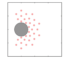
To investigate the impact of the number and arrangement of probes on control effectiveness, we employ rectangular and fan-shaped probe arrangements. The probe locations for the rectangular arrangement method are illustrated in figure 5, with the number of probes varied from 16 to 32. Notably, probes are selected in the region of $x/D < 2$ as acquiring information about more distant flow fields in practical conditions is challenging, and the flow closer to the cylinder significantly influences the lift coefficient ($C_l$) and drag coefficient ($C_d$); see figures 5 and 6.

Figure 5. Location of probes using the rectangular arrangement method.

Figure 6. Location of probes using the fan-shaped arrangement method.

Figure 7 displays the results for the rectangular probe arrangement. It is evident that, in all cases, both $\bar {C}_d$ and $\sigma$ are effectively suppressed, and this suppression amplifies with an increasing number of probes. A similar trend is observed for the fan-shaped arrangement, although the reduction in both $\bar {C}_d$ and $\sigma$ is not as pronounced as in the rectangular arrangement with an equivalent number of probes. This discrepancy may arise from the rectangular arrangement capturing more information in the $x$-direction compared with the $y$-direction.

Figure 7. (a) Time-averaged drag coefficient $\bar {C}_d$ and (b) standard deviation of the drag coefficient $\sigma$ as the number of probes $N_p$ is varied, arranged in a rectangular shape. The grey dashed lines represent the performances of the baseline.

However, figure 8 demonstrates that, with the increasing number of probes ($N_p$) in the fan-shaped arrangement, $\bar {C}_d$ remains nearly constant, whereas $\sigma$ exhibits oscillations, decreasing as $N_p$ increases. One possible explanation for this non-convergence is that the number of probes should be increased further or different locations around the cylinder contribute unevenly to the control effects. Therefore, we employ a rectangular arrangement for our subsequent investigation to address these issues and achieve more stable control effects. This alternative arrangement allows for a more uniform distribution of probes around the cylinder, potentially leading to better data acquisition and more effective control.

Figure 8. (a) Time-averaged drag coefficient $\bar {C}_d$ and (b) standard deviation of the drag coefficient $\sigma$ as the number of probes $N_p$ is varied, arranged in a fan shape. The grey dashed lines represent the performances of the baseline.

3.3. Control trajectories

To elucidate the evolution of the control strategy during the update processes, trajectories of the control strategy (depicted as $\bar {C}_d$ vs $\overline {|Q^*|}$ curves) are presented in figure 9 for periods 21 to 84 with varying numbers of probes. In our control strategy, the cylinder undergoes random control from the 21st to the 30th period, generated by $((rand()\%10)/51.0204-0.0882)/10$, and data from these random actions is utilised to initialise the closed-loop control parameters at the 30th period. Across all cases, both $\overline {|Q^*|}$ and $\bar {C}_d$ decrease gradually over successive periods after a certain duration of DMD control, underscoring the efficacy of parameter matrix updates in enhancing the efficiency of closed-loop control.

Figure 9. Trajectories of the mean drag coefficient during the control process with different numbers of probes. Panel ( f) shows trajectories with 32 probes in region III.

The trajectories can be broadly divided into three regions. In region I, $\bar {C}_d$ experiences a sharp reduction, albeit with occasional instances of it surpassing the baseline. Moving into region II, the rate of decrease in $\bar {C}_d$ diminishes, but stability improves. Notably, in this region, $\overline {|Q^*|}$ registers a significant decrease, indicating an effective reduction in energy injection to the system by the two jets. region II is thus instrumental in enhancing control efficiency. Transitioning to region III, both $\bar {C}_d$ and $\overline {|Q^*|}$ stabilise within a relatively narrow range. In some cases, the control strategy may follow a trajectory as shown in figure 9( f), wherein $\overline {|Q^*|}$ initially increases to reduce $\bar {C}_d$ but subsequently returns to its original position due to a much smaller energy injection compared with energy conservation.

The effect of increasing the number of probes on control becomes evident in figure 9. First, an increase in probes correlates with a notable reduction in $\bar {C}_d$. Second, the augmented probe count leads to a decline in energy injection by the jets, signifying improved control efficiency. Finally, as depicted in figure 9, the rise in probes enables control trajectories to enter region II in fewer periods, thereby enhancing the stability of the control process.

To comprehensively understand control strategies within the three identified regions, the wavelet transforms of $Q^*$ are presented in figure 10. The time–frequency characteristics in region I are particularly distinctive among the three regions. Initially, in region I, the time–frequency characteristics exhibit a noisy signal with no dominant frequency. As the control strategy undergoes updates, the frequency of $Q^*$ gradually concentrates at one or two frequencies near $f^* = 1$.

Figure 10. Wavelet transforms of $Q^*$ in three distinct regions using different numbers of probes.

In contrast, there is minimal disparity between the time–frequency characteristics of regions II and III, as indicated by the stabilisation of the frequency of $Q^*$ at one or two frequencies around the fixed $f^* = 1$. The differentiating factor lies in the emergence of high-frequency information with a duration of $T^*=5\hbox{--}10$ in region III, specifically in cases with 26 and 32 probes. This temporal occurrence aligns with the aforementioned ‘increasing’ and ‘returning’ of $Q^*$, suggesting that the increase in the energy injection by the jets is associated with the introduction of additional frequencies.

3.4. Control efficiency

In the case of active control, efficiency is a crucial factor, and it heavily relies on the applied control method. While the aforementioned control trajectory provides some insight into efficiency, it does not consider the pressure work. To address this, we use the following equation to calculate the efficiency (Choi et al. 2008):

(3.2)\begin{equation} \eta_2=\frac{(F_{Db}-F_{Dc})u_\infty}{\displaystyle 2\int_{t_0}^{t_0+T} \int_A(|0.5\rho\phi^3|+|p_w\phi|)\, {\rm d} A\, {\rm d} t/T}, \end{equation}

where $F_{Db}$ and $F_{Dc}$ represent the drag forces on the cylinder without and with control, respectively. The variable $A$ denotes the upper jet surface where the control is applied, $\rho$ is the fluid density, $p_w$ is the upper jet surface pressure and $\phi$ is the control velocity. The control method is deemed sufficiently efficient when $\eta _2 \gg 1$, even when accounting for additional losses within the control device mechanism (Choi et al. 2008).

Figure 11 illustrates the control efficiency in region III relative to the number of probes. All examined cases exhibit efficiencies well above 1, with even the lowest efficiency reaching 16.7. This suggests that the control method is highly efficient. Furthermore, there is a notable enhancement in control efficiency with an increase in the number of probes, aligning with the observed phenomena in the control trajectories described above.

Figure 11. Control efficiency in region III as a function of the number of probes.

3.5. Computing resource

While the advantages of increasing the number of probes have been elucidated above, it is noteworthy that the augmented number of probes elevates the dimension of the coefficient matrix, potentially leading to increased computational resource consumption during the update processes. All computations in this study are performed on an AMD EPYC 7H12 processor (64-core @2.6 GHz). Specifically, one core is employed, and both the parameter matrix updates and the computation of the LQR in closed-loop control are implemented within the codedFixedValue type boundary conditions.

Throughout the control duration, the parameter matrices undergo significant changes in region I. Notably, the absence of substantial differences between regions II and III, as discussed previously, implies that the updating of coefficient matrices essentially concludes from region II onwards. Consequently, we investigate the time at which the control trajectory enters region II and the computational time required for this process. As depicted in figure 12, $T_{r2}$ exhibits a marked decrease with an increasing number of probes. Simultaneously, the dimension of the parameter matrix increases, causing $T_c$ to initially decrease and then increase with the rising number of probes. The minimum value for $T_c$ is reached when the number of probes is 23.

Figure 12. Normalised time of trajectory entry into region II ($T_{r2}$) and its calculation time ($T_c$) vs the number of probes.

In recent times, DRL has garnered substantial attention, prompting an exploration of its comparative efficacy with the method proposed in this study. Wang et al. (2022), utilising a mesh comprising 16 200 triangular elements, 149 probes and 20 cores for computation, achieved a stable control state after 83.3 hours, resulting in an $8\,\%$ reduction in $C_D$. Notably, this indicates that the DRL method necessitates an additional 77.97 hours for a marginal $0.56\,\%$ increase in the reduction rate, compared with the methodology applied in this paper. Moreover, Rabault et al. (2019), using a mesh comprising 9262 triangular elements, 149 probes and 1 core for computation, reached a stable control state after 24 hours, resulting also in an $8\,\%$ reduction in $C_D$. Consequently, it can be inferred that even when juxtaposed against DRL methods implemented in Python, the approach presented in this study showcases advantages in terms of computational resource consumption.

However, it is imperative to acknowledge that both Rabault et al. (2019) and Wang et al. (2022) employed a considerably higher number of probes than the present study. This consideration may introduce a bias in the comparison of computational resources. To address this, we adopt the methodology proposed by Wang et al. (2022), utilising the same 32 probes, allocating 4 cores for OpenFOAM, and dedicating 16 cores for the DRL program. As depicted in figure 13, with an episode duration of $T_{max} = 20.0$ (spanning approximately 6.5 vortex shedding periods), the proximal policy optimisation (PPO) agent typically learns the control policy after about 200 episodes, requiring approximately 50 hours, considerably longer than $T_c$ (5.14 hours) for 32 probes. Although $C_D$ is reduced to a greater extent compared with the method used in this study, there is an associated increase in $\sigma$, possibly attributable to an insufficient number of probes to attain stable control. In comparison with other DRL outcomes, the method employed in this study demonstrates a notable advantage in terms of computational resource efficiency. One shortcoming of the present approach compared with RL is the necessity to specify a target value for the probes. This requirement can be problematic in complex, non-periodic situations or in cases where the mean and base flow differ significantly. In such scenarios, this control method may be challenging to design and potentially ineffective.

Figure 13. Illustration of the stability and calculation time of the training procedure using deep reinforcement learning (DRL). The red dashed line represents $T_c$ for 32 probes.

3.6. Drag and lift coefficients

In the baseline scenario (without active control), as shown in figure 14(a), the drag coefficient exhibits a frequency of $f_b = 0.6$ Hz (twice the vortex shedding frequency), where $T^* = t/t_p$ represents normalised time. After reaching a steady state ($T^* > 15$), the time-averaged drag coefficient is $\bar {C}_d = 3.2417$, with a standard deviation of $\sigma _b = 0.0198$. In contrast, under active control, the time-averaged drag coefficient $\bar {C}_d=3.0005$ and standard deviation $\sigma =6.6\times 10^{-4}$ reflect the reductions of mean value and deviation approximately $7.44\,\%$ and $96.67\,\%$, respectively. The primary four stages of control are evident in figure 14(a). Stage 1 occurs for $T^*<21$ when the flow field is not fully developed, prompting the flow rate of jets to be set to zero. Stage 2 transpires between $T^*=21$ and $T^*<23$, during which the flow rate of jets is set to a random number between $-$0.021 and 0.021. The data from $T^*=21$ to $T^*=23$ are decomposed by DMDc at $T^*=23$, providing initial system parameters. Stage 3 unfolds between $T^*=23$ and $T^*=40$, wherein the system parameters undergo continuous updating through online DMD. The updated parameters are then employed for closed-loop control. Stage 4 is marked by $T^*>40$ when the flow field is stably controlled. Remarkably, the drag and lift coefficients are effectively controlled after just 17 vortex shedding periods post-application of the control method.

Figure 14. Time variations of (a) drag coefficient $C_d$ and (b) lift coefficient $C_l$ in the case without (baseline curve) and with (controlled curve) active flow control. The effect of flow control is clearly evident.

Similarly, the fluctuation of the lift coefficient is reduced by active control, albeit not as significantly as the drag coefficient. Figure 14(b) illustrates that the standard deviation of the lift coefficient has been reduced from 0.6842 to 0.1014 through active control, representing an $85.18\,\%$ reduction. In contrast, in open-loop scenarios with non-zero net mass injection, $\bar {C}_d=3.1631$ ($2.67\,\%$ reduction) and $\sigma =0.0168$ ($15.15\,\%$ reduction) when $Q^*=0.0011$, proving to be less effective compared with closed-loop control, not to mention the even less-effective control of zero net mass injection with open loop. Thus, it can be concluded that the closed-loop control can achieve significant control effects with only a small flow rate.

Figure 15 portrays the evolution of the normalised mass flow rate $Q^*$ and its time–frequency characteristics, where the frequency is normalised by the baseline vortex shedding frequency. Figure 15(a) shows the evolution of $Q^*$ between $T^* = 90$ and $T^* = 95$, during which $Q^*$ reaches a steady state, fluctuating around 0, with an average absolute value of 0.00102. Figure 15(c) illustrates the spectral characteristics of $Q^*$. The amplitude spectrum of $Q^*$ peaks at one and two times the vortex shedding frequency, mirroring the spectrum of $C_l$. This indicates that the DMDc and DMD online methods used in this study effectively identify the system parameters. Paris et al. (2021) also identified policies involving two frequencies close to the natural vortex shedding frequency. However, the distinction lies in the specific frequencies identified: while the current study found frequencies at 1 and 2.2 times the vortex shedding frequency, both frequencies identified by Paris et al. were below the vortex shedding frequency.

Figure 15. (a) Time variations of the upper jet normalised mass flow rate $Q^*$ and lift coefficient $C_l$ (for $T^*$ from 90 to 95), (b) spectral information of $Q^*$ and (c) spectral information of $C_l$.

3.7. Flow wake characteristics

Figure 16 illustrates the magnitude of velocity with superimposed streamlines for both the baseline and controlled flow. The classic flow field morphology, characterised by the recirculation region behind the cylinder, is evident in the time-averaged flow fields for both cases. This region is confined by two elongated shear layers and terminates with two counter-rotating structures representative of the time-averaged behaviour and position of the shed von Kármán vortices.

Figure 16. Comparison between baseline (a,b) and controlled (c,d) cases in time-averaged magnitude velocity with superimposed streamlines (a,c) and transient magnitude velocity with superimposed streamlines (b,d).

As investigated by Nair et al. (2021) and Paris et al. (2021), the drag reduction arises from the delay in vortex shedding, leading to the generation of ‘elongated vortex structures’. These structures are observable in both transient and time-averaged magnitude velocities. To quantify the elongation of the two counter-rotating vortices, we employ the vortex formation length ($L_f$) at the onset of vortex shedding, as defined by Chopra & Mittal (2019). The vortex formation length is the streamwise distance from the centre of the cylinder to the point along the wake axis where the time-averaged kinetic energy $\overline {e'}$ is maximum; here, $e'(x,t)=\frac {1}{2}u'(x,t)u'(x,t)$. For the baseline and controlled flow, the vortex formation lengths are $L_{fb} = 1.8619$ and $L_{fc} = 6.5$, respectively. This indicates that the elongation rate of $L_{fb}$ has been extended by up to $249.11\,\%$.

It is worth noting that $L_{fb}$ does not seem to correspond to the length of the separation bubble, as shown in figure 16(c). This discrepancy is attributed to a substantial alteration in the flow field morphology induced by active control. As observed in figures 16(c) and 16(d), the wake flow of the baseline exhibits alternately shedding vortex structures, a feature not evident in the controlled wake flow. In the controlled flow, this is replaced by two consistently existing separation bubbles. These separation bubbles interact with each other and alternately shed small vortex structures in the region around $x = 4$–6, exhibiting similarities with low Reynolds number cases. Perhaps, it is this stable presence of separation bubbles that leads to the significant suppression of fluctuations in lift and drag coefficients.

Figure 17 employs the $Q$-criterion to delineate the vortex locations in the wake of the cylinder. The $Q$-criterion illustrates the spatial distribution of vortices for both baseline and controlled flows, showcasing the von Kármán vortex street. Notably, elongated vortex structures are discernible in figure 17. Concurrently, the $Q$ values near the cylinder approach insignificance, signifying that the elongated vortex structures relocate the vortex centre away from the cylinder.

Figure 17. Comparison between baseline (a,b) and controlled (c,d) cases in transient vortex visualisation by $Q$-criterion. Panel (c) corresponds to the time of maximum lift coefficient $C_l$ and panel (d) corresponds to the time of minimum lift coefficient $C_l$.

Figure 18 presents a comparison of pressure distributions between baseline and controlled flow. In contrast to the time-averaged pressure, the active control noticeably diminishes the low-pressure region near $x/D = 1.8$ in the wake of the cylinder. This reduction in low-pressure areas contributes to the decrease in drag coefficients. The two jets induce a redistribution of pressure in the flow field, resulting in a more favourable pressure distribution.

Figure 18. Comparison between baseline (a,b) and controlled (c,d) cases in time-averaged pressure (a,c) and transient pressure (b,d).

The shedding of vortices in an alternating up-and-down pattern creates alternating upper and lower low-pressure regions, as depicted in figure 18(b). These alternating pressure zones are a significant factor in the fluctuation of lift coefficients. Active control effectively suppresses the formation of these alternating pressure regions, leading to a reduction in the fluctuation of lift coefficients.

While there remains a difference in length between the upper and lower low-pressure areas, as illustrated in figure 18(d), this discrepancy is substantially mitigated compared with the baseline configuration. This reduction in the difference between upper and lower low-pressure areas contributes to the overall decrease in lift coefficient fluctuations.

To conduct a detailed analysis of the impact of active control on the flow field, we utilise DMD to decompose both the baseline and controlled flows (within the region of $x/D < 9$). The results are presented in figures 19–22.

Figure 19. Growth rate vs normalised frequency $f^*$ (normalised by vortex shedding frequency) of different DMD modes, sorted by energy: (a) baseline flow and (b) controlled flow.

Figure 19 illustrates the growth rate vs normalised frequency $f^*$ (normalised by vortex shedding frequency) for various DMD modes, sorted by energy. Mode 1, possessing the highest energy, represents the average mode of the flow field with a frequency of 0. Subsequent modes exhibit a conjugate mode with an equal growth rate and an opposite frequency. Modes 2 and 3 have normalised frequencies $f^* = 1$, indicating their representation of von Kármán vortex shedding. Similarly, modes 2, 4, 6, 8 and 10 correspond to the second, third, fourth and fifth harmonics, respectively.

A notable distinction from the baseline is observed, as the original vortex shedding mode transforms into two modes with the same frequency but different growth rates. This alteration is likely attributed to the combined effects of the jets and the cylinder. We consider that this set of negative growth rates is caused by a decrease in the mass flow rate of jets, which can be observed in figure 9. Furthermore, the vortex shedding frequency in the controlled flow doubles compared to the original frequency. In addition, a new average mode and two modes with a normalised frequency $f^* = 4.5$ emerge in the controlled flow.

Figure 20 illustrates the relative energy distribution at various frequencies, encompassing the first 13 orders for baseline flow and 18 orders for controlled flow of DMD modes. The energy values are normalised by the total turbulent kinetic energy, excluding modes above 4000 order and modes with a frequency of 0.

Figure 20. Relative energy distribution at different frequencies of the first 13 orders for baseline flow and 18 orders for controlled flow of DMD modes.

In the baseline flow, turbulent kinetic energy predominantly concentrates at the frequency associated with von Kármán vortex shedding and its octave. Upon comparison with the baseline flow, the controlled flow exhibits a distinct distribution, with turbulent kinetic energy primarily concentrated in modes corresponding to $f^* =2, 4, 4.5, 6$, etc.

Figures 21 and 22 depict the DMD modes, calculated for both the $x$ and $y$ directions, corresponding to the controlled flow and baseline, respectively. As mentioned above, modes 2 to 12 of the baseline characterise von Kármán vortex shedding and its harmonics. In addition, it can be seen from figure 22 that a relatively strong coherent structure persists even in the wake close to the cylinder, contributing to the periodic drag and lift forces experienced by the cylinder.

Figure 21. DMD modes of controlled flow (calculated in both $x$ and $y$ directions) with $T^*\in [90,105]$. Conjugate and average modes are not shown.

Figure 22. First 12 DMD modes of baseline flow (calculated in both $x$ and $y$ directions) with $T^*\in [90,105]$. Conjugate and average modes are not shown.

In contrast to the baseline, the coherent structure in the controlled flow exhibits greater complexity. As seen in figure 21(a,c,e,f), modes 2, 7, 15 and 23 encapsulate the vortex structures and their harmonics originating from the separation bubbles. For those modes, there is no pronounced coherent structure in the vicinity of the wake within the region of $x/D < 4$. Mode 4, shown in figure 21, featuring a frequency of $f^* = 0$, corresponds to an average mode. The morphology of mode 4 reveals that the coherent structure initiates at 90$^\circ$ and 270$^\circ$ of the cylinder, converging at $x/D = 4$ and progresses towards the rear of the flow field. Thus, it is plausible to assert that mode 4 represents the average mode resulting from the expulsion and suction effects of the upper and lower jets. Similarly, mode 11 exemplifies the coherent structure formed by the jets. Notably, this coherent structure is observed at the periphery of the separating bubble, engaging with it and thereby suppressing the detachment of the separating bubble. This coherent structure likely dissipates around $x/D = 6$, coinciding with the vortex formation length at the onset of vortex shedding ($L_f$).

3.8. Robustness with a perturbed upstream flow

In this section, we further verify the robustness of our strategy in a perturbed upstream flow. First, as shown in figure 23, we superpose a travelling wave perturbation to the velocity of the inlet:

(3.3)\begin{equation} u_p(y,T^*)=\frac{3(H/2-y)(H/2+y)(8+\sin(8{\rm \pi} (H/2+T^*/0.3-y)/H))}{4H^2}, \end{equation}

which represents a travelling wave with an amplitude of $u(y)/8$, a wavelength of $H/4$ and a period of $H/4$, added to the original parabolic velocity entrance distribution described by (2.1). Integrating (3.3) over $y$: $\int _{-H/2}^{H/2}u_p(y,t)=H-{3H\sin ((8{\rm \pi} t)/H)}/{128{\rm \pi} ^2}$, since $3H$ is much smaller than $128{\rm \pi} ^2$, it can be assumed that $Re$ is constantly equal to 100. In addition, to study the control behaviour for off-design conditions, $Re$ is raised to 150 at $T^* = 90$, i.e.

(3.4)\begin{equation} u_{tp}(y,T^*)= \left\{ \begin{array}{@{}ll} u_p(y,T^*) & T^*<90,\\ 1.5u_p(y,T^*) & T^*\geq90.\\ \end{array} \right. \end{equation}

Figure 23. Horizontal velocity $u_x$ profile of the inlet flow with a travelling wave perturbation. The dashed line shows the boundary of the cylinder.

The perturbed upstream flow introduces multi-frequency information and larger fluctuations (with a standard deviation of $\sigma _{Cd} = 0.0577$) in the drag coefficient $C_d$ of the cylinder, compared with the constant upstream flow, without affecting the average drag significantly ($\bar {C}_d = 3.2446$). As illustrated in figure 24(b), the drag coefficient $C_d$ under baseline conditions at $Re = 100$ exhibits two primary frequencies: $f^* = 2.00$ and $3.255$. These frequencies correspond to twice the vortex shedding frequency $f^* = 1.00$ and the frequency of the perturbed upstream flow $f^* = 4/0.3/H$, respectively.

Figure 24. Robustness tests with a perturbed upstream flow. (a) Time variations of drag coefficient $Cd$ for two different simulations. The red colour denotes the baseflow with $Re=100$ is simulated, which reaches a converged state at around $T^*=35$, after that, the control is implemented. The incoming flow velocity experiences a sudden rise at $T^*=90$, resulting in $Re=150$, with the continuous application of control strategy. The blue colour represents the baseflow with $Re=150$ is simulated, which reaches a converged state at around $T^*=90$, after that, the control is implemented. (b) PSD of drag coefficient $Cd$ in the case of $Re = 100$. (c) PSD of drag coefficient $Cd$ in the case of $Re = 150$.

Through the control method proposed in this study, the mean cylinder drag coefficient $\bar {C}_d$ in perturbed upstream flow at $Re=100$ is reduced by 6.919 %, accompanied by a corresponding reduction in standard deviation $\sigma _{C_d}$ by 6.412 %. Compared with the control effects in § 3.6, the average drag coefficient $C_d$ reduction rate in the perturbed upstream flow shows no significant difference, but the reduction rate in standard deviation is notably smaller compared with that in the steady incoming flow.

Comparing the baseline and controlled power spectral density (PSD) in the case of $Re = 100$, as depicted in figure 24(b), it is evident that the suppression of fluctuations corresponding to the vortex shedding at twice the frequency is pronounced, whereas the suppression effect on fluctuations corresponding to the perturbed upstream flow frequency is limited. One possible reason for this limitation is that the drag fluctuations in the perturbed upstream flow stem from several sources: twice the vortex shedding frequency $f^* = 2.00$, flow field fluctuations on the front side of the cylinder induced by the perturbed upstream flow ($\,f^* = 4/0.3/H$) and flow field fluctuations on the back side of the cylinder also induced by the perturbed upstream flow ($\,f^* = 4/0.3/H$). However, the control method emphasised in this paper is primarily focused on stabilising the wake flow, which may not effectively suppress the flow field fluctuation on the front (upstream) side of the cylinder ($\,f^* = 4/0.3/H$) caused by the perturbed upstream flow.

In the perturbed upstream flow, after $Re$ is tuned to 150 ($T^* > 90$), the control method in this paper achieves a reduction of 12.73 % in the average drag coefficient $\bar {C}_d$ and a reduction of 38.01 % in the standard deviation of the drag coefficient $\sigma _{C_d}$. These effects are comparable to those observed when directly controlling $Re = 150$ perturbed upstream flow (blue lines in figure 24). However, the notable difference is that compared with $Re=150$, the case with $Re=100$–150 reaches the stabilised control state more quickly after $Re$ becomes 150. This observation suggests that the method employed in this study exhibits better robustness under sudden changes in the flow conditions.

There is no significant difference between the flow field with perturbed upstream flow and that with steady incoming flow, so it is not shown here. This similarity highlights the robustness of the present method for wake control in perturbed upstream flow. The vortex formation lengths in the controlled cases are extended for both $Re = 100$ and $Re = 150$. Specifically, the elongation rate of $L_{fb}$ has been extended by up to 108.61 % and 129.65 % for $Re = 100$ and $Re = 150$, respectively.

To further illustrate the effectiveness of this method for control in complex environments, we use a set-up as shown in figure 25. In this configuration, three square columns with a spacing of 0.3 and size $0.1 \times 0.2$ are positioned in front of the main cylinder at $x = -2$, and three additional square columns with jet entrances of 0.1 widths are also included. The velocity of the three jets is

(3.5)\begin{equation} \left.\begin{array}{c} u_{inj}(T^*)=0.3*(\sin(2 {\rm \pi}t)*\sin({\rm \pi} t)+\sin(10{\rm \pi} t)*\sin(20{\rm \pi} t)+\sin^2(4{\rm \pi} t)), \\ t= T^*/0.3, \end{array}\right\} \end{equation}

where the three square columns and the jet provide more complexity to the cylinder's incoming flow. As shown clearly in figure 25, the wake flow is stabilised to a steady state after the control strategy is implemented.

Figure 25. Comparisons of the instantaneous velocity fields for the case with three upstream columns, each embedded with a jet, between (a) the baseline case and (b) the controlled case.

4. Conclusion

This investigation has delved into the application of an online control strategy employing DMD for flow control, with a fixed Reynolds number of $Re = 100$, past a cylinder confined between two walls. The primary objective was to mitigate vortex shedding through the controlled blowing and suction of two synthetic jets on the cylinder. The $x$-direction velocity fluctuations in the wake have been harnessed to determine the mass flow rate of jets, utilising the LQR and online DMD. The study has explored the interplay between control performance and settings, the relationship between force coefficients and jets’ mass flow rate, as well as the influence of jets on the wake flow field morphology.

First, control performance has been evaluated across varying input penalty factors $R$, the number of probes and probe arrangement methods. The penalty factor $R$ ranges from 5 to 100, with penalty factor $Q$ fixed at $I$. Notably, both $\bar {C}_d$ and $\sigma$ exhibit significant reductions for all $R$, with a more pronounced decrease in $\bar {C}_d$ and $\sigma$ observed when $R$ falls within the range of 10 to 50. The choice of the rectangular arrangement method and an increased number of probes further enhances the effectiveness of control, with the reduction in $\bar {C}_d$ and $\sigma$ becoming more prominent. Despite the increased dimension of the parameter matrix due to the rise in the number of probes, the decrease in $T_{r2}$ causes $T_c$ to exhibit a trend of initially decreasing and subsequently increasing. Moreover, a comparison with DRL has highlighted the computational efficiency advantage of the proposed method.

On the other hand, an analysis of the drag coefficient, lift coefficient, flow behaviours and wake characteristics has been conducted for both baseline and controlled flow scenarios (with $R = 50$, using the rectangular arrangement method, and 32 probes). The controlled flow achieves substantial reductions of $7.44\,\%$ in $\bar {C}_d$, $96.67\,\%$ in $\sigma$ and $85.18\,\%$ in the standard deviation of the lift coefficient. In comparison with open-loop control, the closed-loop approach attains more significant effects with a smaller mass flow rate of jets. The consistency observed between the mass flow rate of jets and lift coefficient spectra characteristics underscores the high precision of the proposed method in identifying system dynamics. Notably, the controlled flow manifests two stable separation bubbles in the region of $x\in [0,4]$, contributing to the significant suppression of lift and drag coefficient fluctuations.

Furthermore, an investigation into the effect of active control on flow modes has revealed distinct alterations from the baseline. The original vortex shedding mode transforms into two modes with identical frequencies and different growth rates, attributed to the combined influence of jets and the cylinder. The vortex shedding frequency in the controlled flow doubles compared with the original frequency. In addition, a new average mode and two modes with a normalised frequency $F^* = 4.5$ emerge in the controlled flow, representing coherent structures formed by the jets.

The robustness of the proposed control method has also been tested on two more complicated cases, involving unsteady incoming flows with multiple frequency components. In such situations, we have also demonstrated that it is adaptive to the variations in flow conditions while keeping the model parameters unchanged. Future extensions of this work could explore control under more intricate conditions.