Article contents
Rejoinder to “Comment” by S. J. Brams and M. D. Davis
Published online by Cambridge University Press: 01 August 2014
Abstract

- Type
- Articles
- Information
- Copyright
- Copyright © American Political Science Association 1975
References
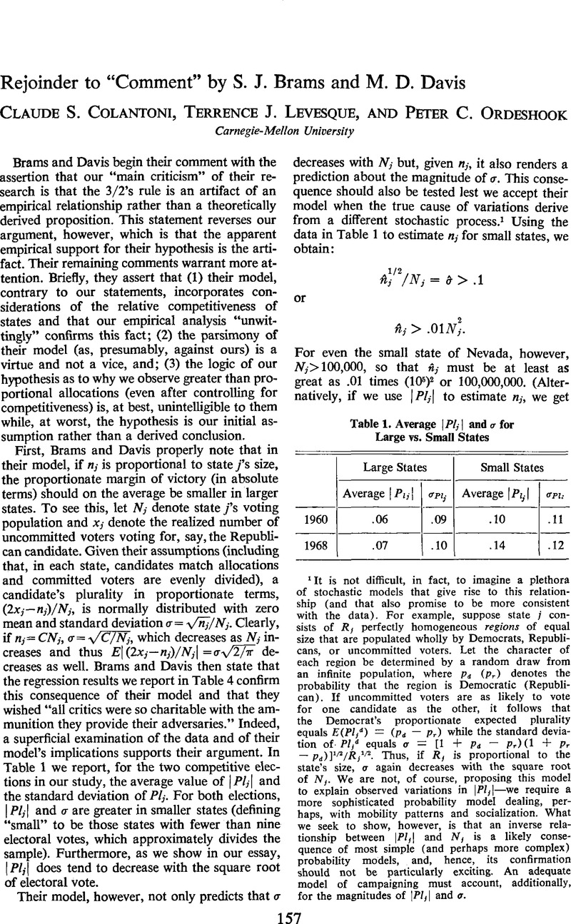
1 It is not difficult, in fact, to imagine a plethora of stochastic models that give rise to this relationship (and that also promise to be more consistent with the data). For example, suppose state j consists of Rj perfectly homogeneous regions of equal size that are populated wholly by Democrats, Republicans, or uncommitted voters. Let the character of each region be determined by a random draw from an infinite population, where pd (pr) denotes the probability that the region is Democratic (Republican). If uncommitted voters are as likely to vote for one candidate as the other, it follows that the Democrat's proportionate expected plurality equals ![]() while the standard deviation of
while the standard deviation of ![]() equals
equals ![]()
![]() . Thus, if Rj is proportional to the state's size, σ again decreases with the square root of Nj. We are not, of course, proposing this model to explain observed variations in ∣Plj∣—we require a more sophisticated probability model dealing, perhaps, with mobility patterns and socialization. What we seek to show, however, is that an inverse relationship between ∣Plj∣ and Nj is a likely consequence of most simple (and perhaps more complex) probability models, and, hence, its confirmation should not be particularly exciting. An adequate model of campaigning must account, additionally, for the magnitudes of ∣Plj∣ and σ.
. Thus, if Rj is proportional to the state's size, σ again decreases with the square root of Nj. We are not, of course, proposing this model to explain observed variations in ∣Plj∣—we require a more sophisticated probability model dealing, perhaps, with mobility patterns and socialization. What we seek to show, however, is that an inverse relationship between ∣Plj∣ and Nj is a likely consequence of most simple (and perhaps more complex) probability models, and, hence, its confirmation should not be particularly exciting. An adequate model of campaigning must account, additionally, for the magnitudes of ∣Plj∣ and σ.
2 Alternatively, suppose that we attribute y per cent of the variation in Plj to violations of the matching hypothesis. Then even if nj = Nj/2, a value for y as low as 10 (per cent) presupposes that the candidates shifted their resources out of the local equilibrium region of the 3/2's rule in those states with ∣Plj ≥ .05 (a majority). That is, to accommodate ten per cent of .05 or more, it must be the case that ∣2pj − 1∣/2 > .05(.1), i.e., either pj < .495 or pj > .505. It is straightforward to show, however, that the small deviations from matching that raise pj to .505 in general lie outside the local equilibrium region.
3 Brams, Steven J. and Davis, Morton D., “The 3/2's Rule in Presidential Campaigning,” American Political Science Review, 68 (March, 1974), 126CrossRefGoogle Scholar.
4 Ibid., p. 132.
5 Ibid., p. 131.
6 Admittedly, our measure of competitiveness is ex post, owing to the unavailability of ex ante data. We do not regard this as serious, however, since it seems reasonable to assume that resources such as trips affect the biases of states less than those biases affect trips (see our note #18) . Ideally, of course, we would prefer an ex ante measure such as the opinions of the candidates themselves as their campaigns commence.
7 To see this we use Brams and Davis's original method of proof: Brams, Steven J. and Davis, Morton D., “Resource-Allocation Models in Presidential Campaigning: Implications for Democratic Representation” Annals of the New York Academy of Sciences, 219 (November, 1973), 105–123CrossRefGoogle ScholarPubMed. Evaluating, as they do, the rate of change in the Republican's expected electoral vote with respect to ri (dWr/dri) at the point.
and letting

we obtain (ignoring all higher order terms in ε),

.
Thus, (a, b) is a local maximum for the Republican only if Ki equals Kj, i.e., only if dWr/dri = 0 for ε = 0 (note that if αi = αj, = 1, expressions (1) and (2) reduce to those seen in the original derivation of the 3/2's rule). The second condition for a local maximum at (a, b) is that dWr/dri < 0 for ε > 0 and dWr/dri > 0 for ε < 0. Setting Ki = Kj, this condition is satisfied (after some rearranging of terms) if and only if
.
Repeating the analysis for the Democrat by letting
.
we find that (αi,a, αjb) is a local maximum for him if and only if Ki = Kj, and
.
Thus, a sufficient condition for [d = (αi,a, αjb), r = (a, b)], to be a local equilibrium in the gametheoretic sense is,
To show now that this is, for all practical purposes, a necessary condition, note that if 1 + 2/ni < αi, or αi </(ni + 2) for two or more states, a local equilibrium cannot exist. There remains, then, two possibilities. First, condition (5) is satisfied for all states but one; second, condition (5) is satisfied for all but two states, with α > 1 + 2/n in one state and α < n/(n + 1) in the other. Suppose state j satisfies the condition and, in particular (to avoid excessive algebra) let αj = nj/(nj, + 2) so that, from condition (4), αi must satisfy αi ≥ ni/(ni + 2). Using the fact that Ki = Kj, expression (3) now requires that

This expression is readily reduced by noting that the maximum value of
is one and that
equal in this instance to
increases as nj increases and closely approximates 1 for relatively small values of nj (e.g., for nj = 12, it equals .968). Adding without proof the condition for αj = 1 + 2/nj, we conclude that in the one or two remaining states, the maximum admissable bounds on αi are,
where ![]() . Note, however, that the bounds on αi, must hold for all j ≠ i, in which case the maximum value presently for
. Note, however, that the bounds on αi, must hold for all j ≠ i, in which case the maximum value presently for ![]() is about 2. Clearly, then, the second term in the expression for Γ is, for reasonable values of ni, several orders of magnitude smaller than one. Thus, we can set Γ = 1 and approximate condition (6) simply by condition (5). To ascertain, then, the maximum admissable discrepancy between R and D, assume that D > R and αi = 1 + 2/ni for all i. Since D = Σri[1 + 2/ni] = R + 2Σ(ri/ni) and
is about 2. Clearly, then, the second term in the expression for Γ is, for reasonable values of ni, several orders of magnitude smaller than one. Thus, we can set Γ = 1 and approximate condition (6) simply by condition (5). To ascertain, then, the maximum admissable discrepancy between R and D, assume that D > R and αi = 1 + 2/ni for all i. Since D = Σri[1 + 2/ni] = R + 2Σ(ri/ni) and ![]() , the necessary and sufficient condition for a local equilibrium is,
, the necessary and sufficient condition for a local equilibrium is,
For example, then, if all ni,'s are on the order of 10,000, a local equilibrium exists if and only if 0.9998 ≤ D/R ≤ 1.0002!
8 One objection to this example, perhaps, is that we choose nj too large and that if we let nj = .01Nj or .001Nj, the 3/2's allocation rule is less unstable (although a 1 per cent increase in Missouri's budget at the expense of Vermont remains advantageous even if there are as few as 4,000 uncommitted voters in Missouri). To repeat our earlier argument, however, the problem is that for smaller values of nj, the model is less able to accommodate the apparent biases of states. Thus, the model is either irrelevant or incomplete from a practical perspective or the instability of a 3/2's rule vitiates its function as a “reference point.”
9 Brams and Davis's objection to the statement (in our abstract) that “the unit rule … is the predominant cause of bias” is legitimate. We perhaps overstated the case there, however, in satisfying the restrictions on an abstract's length. We suggest that they read the conclusion to our essay for a more complete account of our argument, which is simply that “even without weighted voting we should anticipate some variation in resource allocations” across units.
- 6
- Cited by


Comments
No Comments have been published for this article.