Bragg scattering of nonlinear surface waves by sinusoidal sandbars

Abstract

Based on the multiple-scale expansion technique, a new set of extended nonlinear Schrödinger (ENLS) equations up to the third order is derived to account for the additional high-order bottom and dispersion effects as well as the nonlinear wave interaction on wave transformation over periodic sandbars of sinusoidal geometry. By employing the small-amplitude wave assumption, a closed-form analytical solution for Bragg scattering is obtained from the linearised ENLS equations, which demonstrates that a downshift of wave frequency of the maximum reflection is mainly due to the inclusion of the high-order bottom effect. The factors that affect the downshift of the resonant frequency are identified and a theoretical expression in parabolic form is derived to quantify the downshift magnitude. The fully ENLS equations are further analysed to reveal the additional wave nonlinear effects on Bragg scattering characteristics. Under the condition of infinitesimal sandbar amplitude, the ENLS equations render a theoretical expression of the critical value of $kh$ when the nonlinear wave self-modulation effect and the nonlinear wave cross-modulation effect are equal, whereas the former effect is responsible for wavenumber upshifting and the latter downshifting. When $kh$ is larger than the critical value, the increase of wave nonlinearity will enhance the downshift magnitude of the Bragg resonance, and vice versa. For finite amplitude of the bottom sandbar, the ENLS equations are solved numerically to examine the influence of both wave nonlinearity and sandbar amplitude on the characteristics of Bragg resonance. The results reveal that as the increase of sandbar amplitude, the critical $kh$ increases monotonically.

1. Introduction

The Bragg resonance phenomenon, characterised by the partial reflection and transmission of incident waves over sinusoidal sandbars, exhibits the maximal reflection when the wavelength of the incident wave $(\lambda )$ is approximately twice the wavelength of the sandbar undulations $(\lambda _d)$. Initially confirmed in the laboratory by Davies & Heathershaw (1984), the phenomenon was further studied experimentally, particularly in relation to wave–current interactions, by Magne, Rey & Ardhuin (2005) and Laffitte et al. (2021). The higher-order Bragg resonance under more complex resonance conditions has been investigated by Guazzelli, Rey & Belzons (1992) and Peng et al. (2019) through experimental measurements. The Bragg resonance phenomenon has usually been utilised to design artificial bars for coastal protection (Mei, Hara & Naciri 1988; Kirby & Anton 1990; Liu, Luo & Zeng 2015).

Wave scattering theories have been widely used to explain the Bragg resonance phenomenon. The full nonlinear potential flow theory, incorporating surface and bottom nonlinearity, is capable of accurately describing wave scattering. However, numerical approaches are required to solve the equations, as shown by Liu & Yue (1998) and Peng et al. (2019). To explore the analytical solutions or obtain simplified models, other water wave equations with different assumptions are employed. Starting from the surface-linearised Laplace equation, the analytical solutions including Floquet solutions (Howard & Yu 2007; Yu & Howard 2012) and perturbation solution (Davies & Heathershaw 1984) are derived.

By further assuming a wavenumber varying with water depth, the surface-linearised Laplace equation can lead to the mild-slope-type equations (Berkhoff 1973; Kirby 1986a; Chamberlain & Porter 1995). Kirby (1986a) developed extended mild-slope equations by dividing the seabeds into two components that vary slowly and rapidly, which provided an effective method to deal with arbitrary geometries of one- and two-dimensional topography directly. In addition, the mild-slope-type equation has been extended to include the third-order nonlinear effect for Stokes waves where only the forward mode is considered (Kirby & Dalrymple 1983, 1984). These works have been further extended to incorporate the effect of third-order coupling between incident and reflected waves (Liu & Tsay 1984; Kirby 1986b). In particular, Kirby (1986b) used a Lagrangian formulation and derived new nonlinear coupling equations for a weakly nonlinear Stokes wave, which provided an effective and accurate model for both normal and oblique incidence conditions. The mild-slope-type equations are effective when the sandbar amplitude and its variation are mild, where series form solutions have been formulated for wave scattering problems as demonstrated by Liu, Li & Lin (2019), Liu & Zhou (2014) and Fang, Tang & Lin (2023). Recently, Liang et al. (2020) combined the mild-slope equation with the Mathieu instability theorem and derived a formula for phase downshift of Bragg resonance given the infinite bottom length condition. Alternatively, the Boussinesq equation, as an integral model, can be used to describe weak nonlinearity wave propagation over varying topography in shallow water (Madsen, Fuhrman & Wang 2005; Gao et al. 2021), while numerical solution is usually the only viable access.

To derive the analytical solutions for wave scattering over varying topography, not restricted to the shallow-water condition, Mei (1985) developed wave envelope equations based on the multiple-scale expansion to analyse Bragg scattering by sandbars. The equations and solutions were subsequently extended to oblique incidence (Mei et al. 1988; Kirby 1993), doubly sinusoidal ripples (Rey, Guazzelli & Mei 1996), including the current effect (Kirby 1988; Ardhuin & Magne 2007) and random waves with an irregular bottom (Ardhuin & Herbers 2002). Furthermore, the approach of Mei (1985) was further extended to linear Schrödinger equations by Hara & Mei (1988) to include higher-order effects of bottom and dispersion to investigate wave-envelope evolution. Although their equations have difficulties to propose exact solutions for incident and reflected wave amplitudes due to the introduction of additional boundary conditions for continuity of pressure, their analysis demonstrated the importance of the higher-order effects of the bottom and dispersion on Bragg scattering. However, nonlinear wave interaction, which is known to be an influential factor that affects wave reflection by modifying wave speed and producing nonlinear behaviours, are difficult to express in the linear Schrödinger equations of Hara & Mei (1988).

The nonlinear Schrödinger (NLS) equation was initially designed for nonlinear waves propagation over a constant water depth (Benjamin & Feir 1967; Lake et al. 1977). In addition, the NLS has been extended to include wave–current or wave–wave interactions, as shown in Thomas, Kharif & Manna (2012) and Liao et al. (2017). In addition, Onorato, Osborne & Serio (2006) and Hammack, Henderson & Segur (2005) derived the coupled nonlinear Schrödinger (CNLS) equations for a two-wave system, providing the possibility to investigate the effects of nonlinear wave–wave interaction on Bragg scattering. Nevertheless, the NLS equation that directly incorporates all the higher-order bottom effects of sinusoidal sandbars, higher-order dispersion effects and wave nonlinearity, has not been reported yet, likely due to the increased complexity of introducing bottom undulations into two-progressive-wave interactions.

To include high-order effects induced by bottom, dispersion and the nonlinear wave interaction and to explore the underlying mechanisms of physical process of Bragg scattering, a new set of extended nonlinear Schrödinger (ENLS) equations is derived to describe wave scattering over periodic sinusoidal sandbars. This paper is organised as follows. In § 2, the multiple-scale expansion method is utilised to formulate a system of nonlinear equations that considers high-order bottom and dispersion effects, as well as the wave nonlinearity effect. In § 3, analytical solutions for the reflection and transmission rates of the linearised equations are constructed, presenting an analysis of the generation of the wave components, and their mathematical expression in the equations after carefully considering the complex interactions. Subsequently, the causes of the downshift behaviour are elucidated, and a theoretical formula for the downshift magnitude of the Bragg resonance is derived. In § 4, a numerical approach to the full ENLS equations is implemented to further examine the influence of the wave nonlinearity on the Bragg resonance.

2. Mathematical derivation

2.1. Derivation of the coupled model

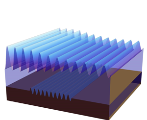
In this section, the ENLS equations up to third order are derived to consider the additional high-order bottom, dispersion effects and nonlinear wave interactions on wave transformation over spatially periodic cosine sandbars. As depicted in figure 1, waves propagate over cosine sandbars with an averaged water depth of $h$ below the mean water surface, with $D$ and $k_d$ representing the amplitude and wavenumber of sandbars, respectively. The bottom wavelength $\lambda _d=2 {\rm \pi}/ k_d$ is the spacing between adjacent peaks from a cosine topography. In addition, waves are assumed to be periodic in both time and space, with $\omega$ and $k$ denoting the wave angular frequency and wavenumber. The waves are allowed to slowly modulate in both time and space scales during the propagation process.

Figure 1. Schematic of the wave propagation domain.

Assuming the weak nonlinearity of waves and topography, we give priority to the problems over $[0, L]$, where the associated parameters, namely, the wave amplitude of incident waves and amplitude of sinusoidal sandbars, are characterised by the same small parameter $\varepsilon$. Here, we denote $\phi$ as the velocity potential function, which satisfies the Laplace equation in the fluid domain,

(2.1)\begin{equation} \frac{\partial ^2\phi }{\partial x^2}+\frac{\partial ^2\phi }{\partial z^2}=0\quad(-h+\sigma< z<\eta ), \end{equation}

where $\sigma =\sigma (x)$ and $\eta =\eta (x,t)$ are the bottom undulation above the mean bottom and free surface elevation, respectively. On the free surface, the kinematic and dynamic boundary conditions are

(2.2)\begin{equation} \frac{\partial \eta }{\partial t}+\frac{\partial \phi }{\partial x}\frac{\partial \eta }{\partial x}-\frac{\partial \phi }{\partial z}=0 \quad(z=\eta ), \end{equation}

and

(2.3)\begin{equation} \frac{\partial \phi }{\partial t}+g \eta +\frac{1}{2}\left[\left(\frac{\partial \phi }{\partial x}\right)^2+\left(\frac{\partial \phi }{\partial z}\right)^2\right]=0 \quad(z=\eta ). \end{equation}

Equations (2.2) and (2.3) are combined to give

(2.4)\begin{equation} \left(\frac{\partial}{\partial t}+\frac{\partial \eta }{\partial t} \frac{\partial}{\partial z}\right)\left\{\frac{\partial \phi }{\partial t}+\frac{1}{2}\left[\left(\frac{\partial \phi }{\partial x}\right)^2+\left(\frac{\partial \phi }{\partial z}\right)^2\right]\right\}+g \phi_z-g\frac{\partial \phi }{\partial x}\frac{\partial \eta }{\partial x}=0\quad (z=\eta ). \end{equation}

On the bottom, the no-flux boundary condition yields

(2.5)\begin{equation} \frac{\partial \phi }{\partial z}-\frac{\partial \phi }{\partial x}\frac{\partial \sigma }{\partial x}=0\quad (z=-h+\sigma ). \end{equation}

To consider third-order effects on the Bragg resonance, the slow variables up to the second order are introduced to capture the higher-order effects of sinusoidal bottom and wave–wave interactions:

(2.6a–d)\begin{equation} \xi _1=\varepsilon x,\quad\xi _2=\varepsilon ^2 x, \quad \tau _1=\varepsilon t,\quad\tau _2=\varepsilon ^2t. \end{equation}

The multiple-scale expansions for $\phi$ and $\eta$ with third-order accuracy give

(2.7)\begin{equation} \phi =\varepsilon \phi _1+\varepsilon ^2 \phi _2+\varepsilon ^3 \phi {}_3+O(\varepsilon ^4) \end{equation}

and

(2.8)\begin{equation} \eta =\varepsilon \eta _1+\varepsilon ^2 \eta _2+\varepsilon ^3 \eta {}_3+O(\varepsilon ^4) \end{equation}

in which $\phi _1=\phi _1(x, z, t, \xi _1, \tau _1, \xi _2, \tau _2), \eta _1=\eta _1(x, t, \xi _1, \tau _1, \xi _2, \tau _2)$, etc. Here $O(\ )$ is an infinitesimal of the same order. Notably, in comparison with the second-order analysis of Mei (1985), we utilise a third-order expansion and introduce two additional slow variables, $\xi _2$ and $\tau _2$, to consider a third-order problem. In addition, we take into account the nonlinear effect in the surface boundary condition, accounting for wave–wave interactions and higher-order bottom and dispersion effects.

By substituting the solutions of (2.7) and (2.8) into (2.1) and utilising the boundary conditions of (2.3), (2.4) and (2.5) with Taylor series expansions at $z=0$ (for (2.3) and (2.4)) and $z=-h$ (for (2.5)), boundary value problems (BVPs) can be obtained for each order of $\varepsilon$ upon separation of the different orders.

2.1.1. First-order problem

The first-order problem is composed of waves propagating both forwards and backwards, as Mei (1985) demonstrated, and an additional non-propagative mode, $B$, which represents the wave-induced mean flow and is generated in the process of nonlinear wave modulations in slow spatial and time scales (Thomas et al. 2012). Considering the significant influence of term $B$ on stability of wave modulation (Thomas et al. 2012; Francius & Kharif 2017; Dhar & Kirby 2023), wave kinematic and dynamic properties (Pizzo et al. 2023), and the geometry of the fluid particle trajectories (Wang, Guan & Vanden-Broeck 2020), we included this term in the present study.

Assuming the associated potential and surface elevation can be expressed as

(2.9)\begin{equation} \phi_1=\left(\psi^+ A^+ S^++\psi^- A^- S^-+\text{c.c.}\right)+B, \end{equation}

and

(2.10)\begin{equation} \eta_1=\tfrac{1}{2}A^+ S^++\tfrac{1}{2}A^- S^-+\text{c.c.}, \end{equation}

where c.c. denotes the conjugate component. The superscripts $+$ and $-$ refer to the incident and reflected waves, respectively. Here $\psi ^{\pm }$ are the corresponding vertical profiles,

(2.11)\begin{equation} \psi ^{{\pm} }=-\frac{g \textrm{i}}{2 \omega }\frac{\cosh k (z+h)}{\cosh kh}. \end{equation}

We use $A^+$ and $A^-$ to denote the complex wave amplitudes, and $B$ is a function, modulated by the slow variables,

(2.12a,b)\begin{equation} A^{{\pm} }=A^{{\pm} }\left(\xi _1,\tau _1,\xi _2,\tau _2\right),\quad B^{{\pm} }=B^{{\pm} }\left(\xi _1,\tau _1,\xi _2,\tau _2\right). \end{equation}

Here $S^+$ and $S^-$ are functions of phases,

(2.13)\begin{equation} S^{ {\pm}}=\exp( {\pm} {\rm i}k x-{\rm i}\omega t). \end{equation}

We use $\omega$ to denote the angular frequency that satisfies the dispersion equation, $\omega =g k \tanh kh$, while the wavenumber $k$ should satisfy the standard Bragg resonance condition established by Mei (1985) to accurately capture wave reflection in the vicinity of the resonance,

(2.14)\begin{equation} k=\tfrac{1}{2}k_d. \end{equation}

Thus, the cosine topography can be expressed in terms of the wavenumber $k$

(2.15)\begin{equation} \sigma=D \cos 2 k x. \end{equation}

2.1.2. Second-order problem

At $O(\varepsilon ^2)$, the BVP can be represented by the following system of equations

(2.16)\begin{gather} \frac{\partial ^2\phi _2}{\partial x^2}+\frac{\partial ^2\phi _2}{\partial z^2}=T_2\quad (-h< z<0), \end{gather}

(2.17)\begin{gather} \frac{\partial ^2\phi _2}{\partial t^2}+g\frac{\partial \phi _2}{\partial z}=P_2\quad (z=0), \end{gather}

(2.18)\begin{gather} \frac{\partial \phi _2}{\partial z}=W_2\quad (z=-h), \end{gather}

(2.19)\begin{gather} \eta _2=R_2 \quad(z=0), \end{gather}

where $T_2, P_2, W_2$ and $R_2$ are compulsory components consisting of lower-order terms, which can be expressed as follows:

(2.20) \begin{align} \left. \begin{aligned} T_2 & =-2 \frac{\partial^2 \phi_1}{\partial x \partial \xi_1} =-\frac{g k}{\omega} \frac{\cosh k(z+h)}{\cosh k h}\left(\frac{\partial A^+}{\partial \xi_1} S^+-\frac{\partial A^-}{\partial \xi_1} S^-\right)+\text{c.c.},\\ P_2 & =\left(-2 \frac{\partial^2 \phi_1}{\partial t \partial \tau_1}- \frac{\partial \eta_1}{\partial t} \frac{\partial^2 \phi_1}{\partial z \partial t}-\frac{\partial \phi_1}{\partial z} \frac{\partial^2 \phi_1}{\partial z \partial t}-\eta_1 \frac{\partial^3 \phi_1}{\partial z \partial t^2}-g \eta_1 \frac{\partial^2 \phi_1}{\partial z^2}+g\frac{\partial \eta_1}{\partial x} \frac{\partial \phi_1}{\partial x}-\frac{\partial \phi_1}{\partial x} \frac{\partial^2 \phi_1}{\partial x \partial t}\right)\bigg|_{z=0}\\ & =g\left(\frac{\partial A^+}{\partial \tau_1} S^++\frac{\partial A^-}{\partial \tau_1} S^-\right)-\frac{\textrm{i}\left(3 \omega^4+g^2 k^2\right)}{2 \omega} A^+ A^- S_{0,2}^+\\ & \quad -\frac{3 \textrm{i}\left(\omega^4-g^2 k^2\right)}{4 \omega}\left[\left(A^+\right)^2 S_{2,2}^++\left(A^-\right)^2 S_{2,2}^-\right]+\text{c.c.},\\ W_2 & =\left. -\sigma \frac{\partial^2 \phi_1}{\partial z^2} \right|_{z=-h} + \left. \frac{d \sigma}{\textrm{d} x} \frac{\partial \phi_1}{\partial x} \right|_{z=-h}\\ & =-\frac{\textrm{i} D g k^2}{4 \omega \cosh k h}\left(A^- S^++A^+ S^-\right)+\frac{3 \textrm{i} D g k^2}{4 \omega \cosh k h}\left(A^+ S_{3,1}^++A^- S_{3,1}^-\right)+\text{c.c.},\\ R_2 & =-\frac{1}{g}\left\{\frac{\partial \phi_2}{\partial t}+\right. \left.\frac{\partial \phi_1}{\partial \tau_1}+\eta_1 \frac{\partial^2 \phi_1}{\partial z \partial t}+\frac{1}{2}\left[\left(\frac{\partial \phi_1}{\partial x}\right)^2+\left(\frac{\partial \phi_1}{\partial z}\right)^2\right]\right\}\\ & = \frac{\omega^4-g^2 k^2}{4 g \omega^2}\left[A^+\left(A^+\right)^*+A^-\left(A^-\right)^*\right]-\frac{1}{g} \frac{\partial B}{\partial \tau_1}-\left. \frac{1}{g} \frac{\partial \phi_2}{\partial t}\right|_{z=0}\\ & \quad +\left[\frac{\textrm{i}}{2 \omega}\left(\frac{\partial A^+}{\partial \tau_1} S_{1,1}^++\frac{\partial A^-}{\partial \tau_1} S_{1,1}^-\right)+\frac{3 \omega^4+g^2 k^2}{4 g \omega^2} A^+ A^- S_{0,2}^+\right. + \frac{\omega^4+g^2 k^2}{4 g \omega^2} A^+\left(A^-\right)^* S_{2,0}^+\\ & \quad+\frac{3 \omega^4-g^2 k^2}{8 g \omega^2}\left(A^+\right)^2 S_{2,2}^+ + \left.\frac{3 \omega^4-g^2 k^2}{8 g \omega^2}\left(A^-\right)^2 S_{2,2}^-+\mathrm{c.c.}\right], \end{aligned} \right\} \end{align}

in which $S_{m,n}^+$ and $S_{m,n}^-$ denote the phase functions for waves propagating in the forward and backward directions, expressed as

(2.21)\begin{equation} S_{m, n}^{ {\pm}}=\textrm{exp}(\textrm{i}({\pm} m k x-n \omega t)), \end{equation}

in particular, $S^\pm =S_{1,1}^\pm$. By solving (2.16)–(2.18) (detailed in Appendix A), $\phi _2$ can be expressed as

(2.22)\begin{align} \phi_2&=-\frac{g \sinh k(z+h)}{4 \omega \cosh k h}\left[2(z+h)\left(\frac{\partial A^+}{\partial \xi_1} S_{1,1}^+-\frac{\partial A^-}{\partial \xi_1} S_{1,1}^-\right)+\textrm{i} k D\left(A^- S_{1,1}^++A^+ S_{1,1}^-\right)\right]\nonumber\\ &\quad -\frac{3 \textrm{i}\left(\omega^4-g^2 k^2\right)^2}{16 \omega^7 \operatorname{sech} 2 k(z+h)}\left[\left(A^+\right)^2 S_{2,2}^++\left(A^-\right)^2 S_{2,2}^-\right]+\frac{\textrm{i}\left(3 \omega^4+g^2 k^2\right)}{8 \omega^3} A^+ A^- S_{0,2}^+\nonumber\\ &\quad +\frac{\textrm{i} D g k}{4 \omega \cosh k h} \frac{3 g k \cosh 3 k z+\omega^2 \sinh 3 k z}{\omega^2 \cosh 3 k h-3 g k \sinh 3 k h}\left(A^+ S_{3,1}^++A^- S_{3,1}^-\right)+\text{c.c.} \end{align}

Then, from (2.19), $\eta _2$ can be derived,

(2.23)\begin{align} \eta_2&=\frac{\omega^4+g^2 k^2}{4 g \omega^2}\left[A^+\left(A^+\right)^*+A^-\left(A^-\right)^*\right]-\frac{1}{g} \frac{\partial B}{\partial \tau_1}+\left\{\frac{3 D\left(\omega^4-g^2 k^2\right)^2}{32 g^3 k^2 \omega^2}\left(A^+ S_{3,1}^++A^- S_{3,1}^-\right)\right.\nonumber\\ &\quad +\frac{1}{4 g k \omega}\left[2 \textrm{i}\left(g k \frac{\partial A^+}{\partial \tau_1}-h \omega^3 \frac{\partial A^+}{\partial \xi_1}\right)+D k \omega^3 A^-\right] S_{1,1}^+\nonumber\\ &\quad +\frac{1}{4 g k \omega}\left[2 \textrm{i}\left(g k \frac{\partial A^-}{\partial \tau_1}+h \omega^3 \frac{\partial A^-}{\partial \xi_1}\right)+D k \omega^3 A^+\right] S_{1,1}^-\nonumber\\ &\quad \left.-\frac{g k^2\left(\omega^4-3 g^2 k^2\right)}{8 \omega^6}\left[\left(A^+\right)^2 S_{2,2}^++\left(A^-\right)^2 S_{2,2}^-\right]+\frac{\omega^4+g^2 k^2}{4 g \omega^2} A^+\left(A^-\right)^* S_{2,0}^++\text{c.c.}\right\}. \end{align}

As demonstrated in Appendix A, the following solvable conditions must be satisfied:

(2.24)\begin{equation} \int_{-h}^0\left({\mp} \frac{g k}{\omega} \frac{\cosh k(z+h)}{\cosh k h} \frac{\partial A^{ {\pm}}}{\partial \xi_1}\right) \psi^{ {\pm}} \,\textrm{d}z=\left.\left(\frac{\partial A^{ {\pm}}}{\partial \tau_1}\right) \psi^{ {\pm}}\right|_{z=0}-\left.\left(-\frac{\textrm{i} D g k^2}{4 \omega \cosh k h} A^{{\mp}}\right) \psi^{ {\pm}}\right|_{z=-h} \end{equation}

which can be simplified as

(2.25)\begin{equation} \frac{\partial A^{{\pm} }}{\partial \tau _1}+C_g^{{\pm} }\frac{\partial A^{{\pm} }}{\partial \xi _1}+\textrm{i}D_0^{{\pm} }A^{{\mp} }=0 \end{equation}

in which $C_g^\pm$ and $D_0^\pm$ are the group velocities and topography-induced terms,

(2.26)\begin{equation} C_g^{ {\pm}}={\pm}\left(\frac{\omega}{2 k}+h \omega \operatorname{csch} 2 k h\right), \end{equation}

and

(2.27)\begin{equation} D_0^{ {\pm}}=\tfrac{1}{2} D k \omega \operatorname{csch} 2 k h . \end{equation}

in which $D_0^{ \pm }$, with the dimension of frequency, is a forcing term and represents leading-order interaction between the waves and the sandbars, where the forward (backward) mode is reflected by the ripple components, thereby forcing a resonant backward (forward) wave mode. Its expression is identical to earlier work (Mei 1985) for pure wave condition. If we ignore the current effects in the early work of Kirby (1988), the present expressions of $D_0^{ \pm }$ in (2.27) are identical to their results.

2.1.3. Third-order problem

For the third-order problem, the solvable conditions of the singular modes, $S_{1,1}^+$ and $S_{1,1}^-$, and the zero mode are considered in the present solution. The other harmonics in the compulsory terms, which have no association with resonance, are not considered here. The third-order problem for potential function is defined as

(2.28) \begin{equation} \left. \begin{gathered} \frac{\partial^2 \phi_3}{\partial x^2}+\frac{\partial^2 \phi_3}{\partial z^2}=T_{0,0}^{3,+}+\left(T_{1,1}^{3,+} S_{1,1}^++T_{1,1}^{3,-} S_{1,1}^-+\text{c.c.}\right)\quad (-h< z<0),\\ \frac{\partial^2 \phi_3}{\partial t^2}+g \frac{\partial \phi_3}{\partial z}=P_{0,0}^{3,+}+\left(P_{1,1}^{3,+} S_{1,1}^++P_{1,1}^{3,-} S_{1,1}^-+\text{c.c.}\right)\quad (z=0),\\ \frac{\partial \phi_3}{\partial z}=W^{3,+}_{1,1} S_{1,1}^++W^{3,-}_{1,1} S_{1,1}^-+\text{c.c.}\quad (z=-h), \end{gathered} \right\} \end{equation}

in which

(2.29) \begin{align} \left. \begin{aligned} T_{0,0}^{3,+} & =-\frac{\partial^2 B}{\partial \xi_1^2}, \\ T_{1,1}^{3, \pm} & ={\mp} \frac{g \operatorname{sech} k h}{2 \omega}\left\{\vphantom{\frac{\partial^2 B}{\partial \tau_1^2}}2 k \cosh k(z+h) \frac{\partial A^{ {\pm}}}{\partial \xi_2}+D k^2 \sinh k(z+h) \frac{\partial A^{{\mp}}}{\partial \xi_1}\right.\\ & \left.\quad \mp \textrm{i}[2 k(z+h) \sinh k(z+h)+\cosh k(z+h)] \frac{\partial^2 A^{ {\pm}}}{\partial \xi_1^2}\right\},\\ P_{0,0}^{3,+} & =\frac{\omega^4-g^2 k^2}{4 \omega^2} \frac{\partial\left[A^+\left(A^+\right)^*+A^-\left(A^-\right)^*\right]}{\partial \tau_1}+\frac{g^2 k}{2 \omega} \frac{\partial\left[A^+\left(A^+\right)^*-A^-\left(A^-\right)^*\right]}{\partial \xi_1}-\frac{\partial^2 B}{\partial \tau_1^2},\\ P_{1,1}^{3, \pm} & =g \frac{\partial A^{ {\pm}}}{\partial \tau_2}+\frac{\textrm{i} g}{2 \omega} \frac{\partial^2 A^{ {\pm}}}{\partial \tau_1^2} \mp \frac{\textrm{i} h \omega^2}{k} \frac{\partial^2 A^{ {\pm}}}{\partial \xi_1 \partial \tau_1}+\frac{\omega^2 D}{2} \frac{\partial A^{{\mp}}}{\partial \tau_1}-\frac{\textrm{i}\left(\omega^4+g^2 k^2\right)^2}{4 g \omega^3} A^{ {\pm}} A^{{\mp}}\left(A^{{\mp}}\right)^*\\ & \quad +\,\frac{\textrm{ i}\left(9 g^6 k^6-12 g^4 k^4 \omega^4+13 g^2 k^2 \omega^8-2 \omega^{12}\right)}{16 g \omega^7}\left(A^{ {\pm}}\right)^2\left(A^{ {\pm}}\right)^*\\ & \quad +\,\frac{\textrm{i}\left(\omega^4-g^2 k^2\right)}{2 g \omega} A^{ {\pm}} \frac{\partial B}{\partial \tau_1} \pm \textrm{i} g k A^{ {\pm}} \frac{\partial B}{\partial \xi_1},\\ W^{3,\pm}_{1,1} & =\frac{3 \textrm{i} D^2 g k^3 \operatorname{sech} k h\left(3 g k \cosh 3 k h-\omega^2 \sinh 3 k h\right)}{24 g k \omega \sinh 3 k h-8 \omega^3 \cosh 3 k h} A^{ {\pm}}. \end{aligned} \right\} \end{align}

At the order of $\varepsilon ^3$, (A25) yields solvability conditions for singular components, $S_{1,1}^\pm$, by way of the Green formula depicted in (A24)

(2.30)\begin{equation} \int _{-h}^0T_{1,1}^{3,\pm }\psi ^{{\pm} }\,\textrm{d}z=\frac{1}{g}P_{1,1}^{3,\pm }\left.\psi ^{{\pm} }\right|{}_{z=0}-W^{3,\pm}_{1,1}\left.\psi ^{{\pm} }\right|{}_{z=-h}, \end{equation}

which can be further integrated with the substitution of $T_{1,1}^{3,\pm }$, etc., resulting in two coupled equations for $A^+, A^-$ and $B$

(2.31)$$\begin{gather} \frac{\partial A^{{\pm} }}{\partial \tau _2}+C_g^{{\pm} }\frac{\partial A^{{\pm} }}{\partial \xi _2}+ B_1^{{\pm} }\frac{\partial ^2A^{{\pm} }}{\partial \tau _1^2}+B_2^{{\pm} }\frac{\partial ^2A^{{\pm} }}{\partial \xi _1\partial \tau _1}+B_3^{{\pm} }\frac{\partial ^2A^{{\pm} }}{\partial \xi _1^2}+D_1^{{\pm} }\frac{\partial A^{{\mp} }}{\partial \tau _1}+D_2^{{\pm} }\frac{\partial A^{{\mp} }}{\partial \xi _1}\nonumber\\ +D_3^{{\pm} }A^{{\pm} }+\left\{\sigma _1^{{\pm} }\left| A^{{\pm} }\right| ^2+\sigma _2^{{\pm} }\left| A^{{\mp} }\right| ^2+\sigma _3^{{\pm} }\frac{\partial B}{\partial \tau _1}+\sigma _4^{{\pm} }\frac{\partial B}{\partial \xi _1}\right\}A^{{\pm} }=0, \end{gather}$$

in which $| A^{\pm }|$ corresponds the modulus of $A^{\pm }$, given by $\sqrt {A^{\pm }(A^{\pm })^*}$. The coefficients can be expressed as

(2.32)\begin{align} \left. \begin{gathered} B_1^{ {\pm}}=\frac{\textrm{i}}{2 \omega}, B_2^{ {\pm}}={\mp} \textrm{i} h \tanh k h, B_3^{ {\pm}}=-\frac{\textrm{i} h \omega}{2 k} \operatorname{coth} k h, D_1^{ {\pm}}=\frac{D \omega^2}{2 g}, D_2^{ {\pm}}={\pm} \frac{D \omega^3}{4 g k},\\ D_3^{ {\pm}}=\frac{3 g k \cosh 3 k h-\omega^2 \sinh 3 k h}{4 \omega^2 \cosh 3 k h-12 g k \sinh 3 k h} \frac{3 \textrm{i} D^2 k^2 \omega}{\sinh 2 k h},\\ \sigma_1^{ {\pm}}=\frac{\textrm{i} g k^3(20+13 \cosh 2 k h+2 \cosh 4 k h+\cosh 6 k h)}{8 \omega \sinh ^3 2 k h},\\ \sigma_2^{ {\pm}}=-\frac{\textrm{i}\left(\omega^4+g^2 k^2\right)^2}{4 g^2 \omega^3}, \sigma_3^{ {\pm}}=\frac{\textrm{i}\left(\omega^4-g^2 k^2\right)}{2 g^2 \omega}, \sigma_4^{ {\pm}}={\pm} \textrm{i} k. \end{gathered} \right\} \end{align}

The zero mode, $T_{0,0}^{3,+}$, does not depend on $z$. Consequently, combining the Laplace equation, bottom boundary and bottom conditions, the solvable condition for $B$ is derived to fulfil the surface boundary condition,

(2.33)\begin{equation} g h T_{0,0}^{3,+}=P_{0,0}^{3,+}. \end{equation}

By introducing the expressions of $T_{0,0}^{3,+}$, etc., (2.33) is transformed into a hyperbolic partial differential equation

(2.34)\begin{equation} \frac{\partial^2 B}{\partial \tau_1^2}-g h \frac{\partial^2 B}{\partial \xi_1^2}=\frac{\omega^4-g^2 k^2}{4 \omega^2} \frac{\partial\left(\left|A^+\right|^2+\left|A^-\right|^2\right)}{\partial \tau_1}+\frac{g^2 k}{2 \omega} \frac{\partial\left(\left|A^+\right|^2-\left|A^-\right|^2\right)}{\partial \xi_1}. \end{equation}

We multiply (2.25) by $(A^{\pm })^*$ and, upon conjugation and summation, obtain

(2.35)\begin{equation} \frac{\partial\left(\left|A^+\right|^2+\left|A^-\right|^2\right)}{\partial \tau_1}+C_g^+ \frac{\partial\left(\left|A^+\right|^2-\left|A^-\right|^2\right)}{\partial \xi_1}=0, \end{equation}

which indicates that (2.34) can be automatically satisfied by constructing the formulation of

(2.36a,b)\begin{equation} \frac{\partial B}{\partial \tau _1}=-C_g^+\lambda \left(\left| A^+\right| ^2+\left| A^-\right| ^2\right),\quad \frac{\partial B}{\partial \xi _1}=\lambda \left(\left| A^+\right| ^2-\left| A^-\right| ^2\right), \end{equation}

in which

(2.37)\begin{equation} \lambda =\frac{1}{C_g^{+2}-g h}\left(\frac{g^2 k}{2 \omega }-C_g^+\frac {\omega^4 - g^2 k} {4\omega^2}\right). \end{equation}

By introducing the first-order derivatives of $B$ from (2.36a,b) into (2.31), we can eliminate the terms related to it and thereby attain the second set of solvability conditions for $A^\pm$

(2.38)$$\begin{gather} \frac{\partial A^{{\pm} }}{\partial \tau _2}+C_g^{{\pm} }\frac{\partial A^{{\pm} }}{\partial \xi _2}+ B_1^{{\pm} }\frac{\partial ^2A^{{\pm} }}{\partial \tau _1^2}+B_2^{{\pm} }\frac{\partial ^2A^{{\pm} }}{\partial \xi _1\partial \tau _1}+B_3^{{\pm} }\frac{\partial ^2A^{{\pm} }}{\partial \xi _1^2}+D_1^{{\pm} }\frac{\partial A^{{\mp} }}{\partial \tau _1}\nonumber\\ +D_2^{{\pm} }\frac{\partial A^{{\mp} }}{\partial \xi _1}+D_3^{{\pm} }A^{{\pm} }+\left\{F_1^{{\pm} }\left| A^{{\pm} }\right| ^2+F_2^{{\pm} }\left| A^{{\mp} }\right| ^2\right\}A^{{\pm} }=0, \end{gather}$$

in which

(2.39)\begin{align} \left. \begin{gathered} F_1^{ {\pm}}=\frac{\textrm{i} g k^3(20+13 \cosh 2 k h+2 \cosh 4 k h+\cosh 6 k h)}{8 \omega \sinh ^3 2 k h}-\frac{\textrm{i}\left[2 g^2 k \omega+C_g^+\left(g^2 k^2-\omega^4\right)\right]^2}{8 g^2 \omega^3\left[g h-C_g^{+2}\right]},\\ F_2^{ {\pm}}=-\frac{\textrm{i}\left(\omega^4+g^2 k^2\right)^2}{4 g^2 \omega^3}-\frac{\textrm{i}\left[-4 g^4 k^2 \omega^2+\left(\omega^4-g^2 k^2\right)^2 C_g^{+2}\right]}{8 g^2 \omega^3\left[g h-C_g^{+2}\right]}. \end{gathered} \right\} \end{align}

Equation (2.38) can be reduced to the linear Schrödinger equation derived by Hara & Mei (1988), if wave–wave interaction is neglected and the transformations to (2.25) are implemented. However, their equation formulates a partial differential equation with respect to the second-order derivative of the spatial variable $x$, necessitating additional boundary conditions for continuity of pressure, thereby posing a challenge for seeking exact solutions. Therefore, they derived the ratio of the envelope height at antinodes in the strip to the envelope height at the strip's edge to settle for the second best. In the present study, to directly identify the solutions for incident and reflected wave evolutions, the differential transformations on (2.25) are employed to replace the second derivatives with respect to $x$ in (2.38) as follows:

(2.40)\begin{equation} \left. \begin{gathered} \frac{\partial^2 A^{ {\pm}}}{\partial \xi_1^2} \rightarrow-\frac{\textrm{i} D_0^{ {\pm}}}{C_g^{ {\pm}}} \frac{\partial A^{{\mp}}}{\partial \xi_1}-\frac{1}{C_g^{ {\pm}}} \frac{\partial^2 A^{ {\pm}}}{\partial \tau_1 \partial \xi_1},\\ \frac{\partial^2 A^{ {\pm}}}{\partial \tau_1 \partial \xi_1} \rightarrow-\frac{\textrm{i} D_0^{ {\pm}}}{C_g^{ {\pm}}} \frac{\partial A^{{\mp}}}{\partial \tau_1}-\frac{1}{C_g^{ {\pm}}} \frac{\partial^2 A^{ {\pm}}}{\partial \tau_1^2}. \end{gathered} \right\} \end{equation}

We introduce transforms of temporal and spatial scales to recover $x$ and $t$

(2.41a,b)\begin{equation} \varepsilon \frac{\partial }{\partial \tau _1}+\varepsilon ^2\frac{\partial }{\partial \tau _2}\rightarrow \frac{\partial }{\partial t},\quad\varepsilon \frac{\partial }{\partial \xi _1}+\varepsilon ^2\frac{\partial }{\partial \xi _2}\rightarrow \frac{\partial }{\partial x}, \end{equation}

which enables $A^{ \pm }(\xi _1, \tau _1, \xi _2, \tau _2)$ to return to $A^{ \pm }(x, t)$ and, thus, obtain a set of coupled nonlinear equations for $A^+$ and $A^-$, which can be employed to investigate the envelope evolution of waves,

(2.42) $$\begin{gather} \frac{\partial A^+}{\partial t}+C_g^+ \frac{\partial A^+}{\partial x} +\textrm{i} D_0^+ A^-\nonumber\\ +\overbrace{\left(D_1^+-\frac{\textrm{i} B_2^+ D_0^+}{C_g^+}+\frac{\textrm{i} B_3^+ D_0^+}{\left(C_g^+\right)^2}\right) \frac{\partial A^-}{\partial t}+\left(D_2^+-\frac{\textrm{i} B_3^+ D_0^+}{C_g^+}\right) \frac{\partial A^-}{\partial x}+D_3^+ A^+}^{high-order\ bottom\ effect}\nonumber\\ + \underbrace{\left(B_1^+-\frac{B_2^+}{C_g^+}+\frac{B_3^+}{\left(C_g^+\right)^2}\right) \frac{\partial^2 A^+}{\partial t^2}}_{high-order\ dispersion\ effect}+\underbrace{F_1^+\left|A^+\right|^2 A^++F_2^+\left|A^-\right|^2 A^+}_{nonlinear\ wave\ interaction}=0, \end{gather}$$

(2.43) $$\begin{gather} \frac{\partial A^-}{\partial t}+C_g^- \frac{\partial A^-}{\partial x}+\kern1pt\textrm{i} D_0^- A^+\nonumber\\ +\overbrace{\left(D_1^--\frac{\textrm{i} B_2^- D_0^-}{C_g^-}+\frac{\textrm{i} B_3^- D_0^-}{\left(C_g^-\right)^2}\right) \frac{\partial A^+}{\partial t}+\left(D_2^--\kern1pt\frac{\textrm{i} B_3^- D_0^-}{C_g^-}\right) \frac{\partial A^+}{\partial x}+D_3^- A^-}^{\textit{high-order bottom effect}}\nonumber\\ + \underbrace{\left(B_1^--\frac{B_2^-}{C_g^-}+\frac{B_3^-}{\left(C_g^-\right)^2}\right) \frac{\partial^2 A^-}{\partial t^2}}_{\textit{high-order dispersion effect }}+\underbrace{F_1^-\left|A^-\right|^2 A^-+F_2^-\left|A^+\right|^2 A^-}_{\textit{nonlinear wave interaction }}=0. \end{gather}$$

Equations (2.42) and (2.43) are the newly derived ENLS equations, consisting of the basic governing equations of Mei (1985) (the first three items), the bottom effect terms with $D_0^{ \pm }$ representing the first-order bottom effect and $D_1^{ \pm }, D_2^{ \pm }$ and $D_3^{ \pm }$ being second-order bottom effects, the high-order wave dispersion effect terms ($B_1^{ \pm }$, etc.) and the nonlinear terms with $F_1^{ \pm }$ and $F_2^{ \pm }$ related to the wave–wave interactions.

The internal correlations between the newly derived ENLS and the Schrödinger equations are summarised as follows. (1) If the topography-related terms are eliminated and the substitution of $\partial ^2 / \partial t^2$ for $\partial ^2 / \partial x \partial t$ and $\partial ^2 / \partial x^2$ is applied in accordance with the first solvable conditions, the ENLS is reduced to a range of variants of the Schrödinger equation. (2) If the sandbars vanish and water depth is assumed to be infinite, the ENLS can be reduced to the CNLS equations established by Hammack et al. (2005); compared with the CNLS of Onorato et al. (2006), the only slight difference lies on the coefficients $F_2^{ \pm }$. (3) The ENLS can be simplified to the NLS equations of Thomas et al. (2012) and Liao et al. (2017) if the influence of the current is neglected.

3. Exact solution for the linearised ENLS equations

3.1. Derivation of the exact solution

Closed-form solutions for the ENLS equations are difficult to propose due to the nonlinearity derived from the wave–wave interactions. However, by assuming wave amplitudes to be sufficiently small, the equations can be reduced to a linear system coupling $A^+$ and $A^-$, leading to exact solutions, which enables systematic investigation on the influence of topographical factors on Bragg resonance. Therefore, in this section, by neglecting the wave nonlinearity, the linearised ENLS equations are obtained

(3.1)$$\begin{gather} \frac{\partial A^+}{\partial t}+C_g^+ \frac{\partial A^+}{\partial x}+\textrm{i} D_0^+ A^- +\left(B_1^+-\frac{B_2^+}{C_g^+}+\frac{B_3^+}{\left(C_g^+\right)^2}\right) \frac{\partial^2 A^+}{\partial t^2}\nonumber\\ +\left(D_1^+-\frac{\textrm{i} B_2^+ D_0^+}{C_g^+}+\frac{\textrm{i} B_3^+ D_0^+}{\left(C_g^+\right)^2}\right) \frac{\partial A^-}{\partial t}+\left(D_2^+-\frac{\textrm{i} B_3^+ D_0^+}{C_g^+}\right) \frac{\partial A^-}{\partial x}+D_3^+ A^+=0, \end{gather}$$

(3.2)$$\begin{gather} \frac{\partial A^-}{\partial t}+C_g^- \frac{\partial A^-}{\partial x}+\textrm{i} D_0^- A^+ +\left(B_1^--\frac{B_2^-}{C_g^-}+\frac{B_3^-}{\left(C_g^-\right)^2}\right) \frac{\partial^2 A^-}{\partial t^2}\nonumber\\ +\left(D_1^--\frac{\textrm{i} B_2^- D_0^-}{C_g^-}+\frac{\textrm{i} B_3^- D_0^-}{\left(C_g^-\right)^2}\right) \frac{\partial A^+}{\partial t}+\left(D_2^--\frac{\textrm{i} B_3^- D_0^-}{C_g^-}\right) \frac{\partial A^+}{\partial x}+D_3^- A^-=0. \end{gather}$$

As illustrated in figure 1, an incident wave train of both temporally and spatially periodic waves arrives from $x=-\infty$ and these waves are continuously reflected by the bottom sandbars, forming reflected waves that propagate in the reverse direction and produce standing waves by the superposition of the incident and reflected waves. In the region $x>L$, where the varying topography vanishes, only the forward-propagating mode exists, designated as transmitted waves. The region $0< x< L$ is highlighted by periodic sinusoidal bars of amplitude $D$ and wavenumber $2k$, and $L$ is the total length of the sandbars and $N_d=L / \lambda _d$ denotes the number of sandbars.

Let the incident and reflected waves be slightly detuned from the Bragg resonance, with their wave frequencies being $\omega ^+=\omega ^-=\omega +\omega ^{\prime }$, where $\omega ^{\prime }$ implies wavenumber deviations $k^{\prime }$ and $k^{\prime \prime }$ for the incident and reflected waves, respectively. Over the sandbars $0< x< L$, we can find solutions such as

(3.3)\begin{equation} A^+=A_0 T(x) \textrm{e}^{-\textrm{i} \omega^{\prime} t} \quad(0< x< L), \end{equation}

and

(3.4)\begin{equation} A^-=A_0 R(x) \textrm{e}^{-\textrm{i} \omega^{\prime} t} \quad(0< x< L). \end{equation}

Let $\tilde {R}$ denote the reflection coefficient, given by $|R(0)|$. An exact solution for the reflection rate, $\tilde {R}$, can be written as (details can be found in Appendix B)

(3.5)\begin{equation} \tilde{R}=\sqrt{\frac{Q_1^2}{|P \cot PL| ^2+Q_2^2}}, \end{equation}

in which $Q_1, Q_2$ and $P$ are functions of $\omega ^{\prime }$:

(3.6)\begin{equation} \left. \begin{gathered} Q_1=\frac{-\textrm{i}\left\{E_3\left[D_3^++\omega^{\prime}\left(-\textrm{i}+E_2 \omega^{\prime}\right)\right]+C_g^+\left(E_1 \omega^{\prime}+\textrm{i} D_0^+\right)\right\}}{E_3^2-\left(C_g^+\right)^2},\\ Q_2=\frac{E_3 D_0^+-\textrm{i}\left\{E_1 E_3 \omega^{\prime}+C_g^+\left[D_3^++\omega^{\prime}\left(-\textrm{i}+E_2 \omega^{\prime}\right)\right]\right\}}{E_3^2-\left(C_g^+\right)^2},\\ P=\sqrt{\frac{\left(D_3^++\omega^{\prime}\left(-\textrm{i}+E_2 \omega^{\prime}\right)\right)^2-\left(E_1 \omega^{\prime}+\textrm{i} D_0^+\right)^2}{E_3^2-\left(C_g^+\right)^2}}, \end{gathered} \right\} \end{equation}

where $E_1, E_2$ and $E_3$ are coefficients, expressed as

(3.7)\begin{equation} \left. \begin{gathered} E_1=-\frac{\textrm{i} D\left(g^4 h k^4+g \omega^6-h \omega^8\right)}{2\left(g^2 h k^2+g \omega^2-h \omega^4\right)^2},\\ E_2=-\frac{\textrm{i}}{2 \omega}+2 \textrm{i} h \omega \frac{\left(-g+h \omega^2\right)\left(-g^2 k^2+\omega^4\right)}{\left(g^2 h k^2+g \omega^2-h \omega^4\right)^2},\\ E_3=D\left(-\frac{g k}{4 \omega}+\frac{\omega^3}{4 g k}+\frac{g^2 k \omega}{4 g^2 h k^2+4 g \omega^2-4 h \omega^4}\right). \end{gathered} \right\} \end{equation}

It is clear that the only difference between the present solution (3.5) and the solution of Mei (1985) lies in the terms $Q_1$, $Q_2$ and $P$. If the higher-order contributions of $E_1$, $E_2$, $E_3$ and $D_3^+$ are set to zero, the present solution reduces to the solution of Mei (1985),

(3.8)\begin{equation} \tilde{R}_{{M}}=\sqrt{\frac{Q_{1, {M}}^2}{Q_{2, {M}}^2+\left|P_{{M}} \cot P_{{M}} L\right|^2}}, \end{equation}

in which

(3.9a–c)\begin{equation} Q_{1, {M}}=-\frac{D_0^+}{C_g^+}, \quad Q_{2, {M}}=\frac{\omega^{\prime}}{C_g^+}, \quad P_{{M}}=\frac{1}{C_g^+} \sqrt{\left(\omega^{\prime}\right)^2-\left(D_0^+\right)^2}, \end{equation}

where the subscript ${M}$ represents the solution of Mei (1985). $Q_{1, {M}}, Q_{2, {M}}$ and $P_{{M}}$ are even functions with respect to $\omega ^{\prime }$, indicating good symmetry with $\tilde {R}_{{M}}(\omega ^{\prime })=\tilde {R}_{{M}}(-\omega ^{\prime })$ and the maximum reflection occurring at $\omega ^{\prime }=0$. However, as evidenced by the inequalities of $Q_1(\omega ^{\prime }) \neq Q_1(-\omega ^{\prime }), Q_2(\omega ^{\prime }) \neq Q_2(-\omega ^{\prime })$ and $P(\omega ^{\prime }) \neq P(-\omega ^{\prime })$, the present solution is not symmetrically distributed, which could potentially shift the positions of maximum reflection.

3.2. Verifications of the solution for reflection

To verify the analytical solution for reflection in (3.5), experiment-based wave scattering by sinusoidal sandbars is investigated. The geometrical configuration of the experimental set-up is depicted in figure 1. The performance of the present solution is verified by comparing it with the experiments conducted by Davies & Heathershaw (1984) and Laffitte et al. (2021), denoted as D1 and L1, respectively. The wave- and topographic-related parameters of the experiments are shown in table 1.

Table 1. Parameters for wave scattering by sinusoidal sandbars.

Figure 2 shows the comparisons of the reflection $\tilde {R}$ obtained from the present solution, the analytical solution from Mei (1985), the numerical solution of Liu & Yue (1998), and the measured data by Davies & Heathershaw (1984) and Laffitte et al. (2021). The red dotted lines in figure 2(a) signify $2 k^+ / k_d=1$, which is the peak of the Bragg resonance predicted by Mei (1985). However, in practice, a slight phase downshift is commonly observed, as indicated by the numerical solutions of Liu & Yue (1998) and the measured data, which is accurately captured by the present solution. In prior research studies, the downshift characteristics for case D1 were investigated (Madsen et al. 2005; Liang et al. 2020), and the results of these studies are summarised in table 2.

Figure 2. Comparison of the reflection rate $\tilde {R}$ for case-D1 and case-L1 among the present solution in (3.5) (blue solid line), analytical solution from Mei (1985) in (3.8) (red dashed line), numerical solutions of Liu & Yue (1998) (green dots) and experimental data from Davies & Heathershaw (1984) (black circles) and Laffitte et al. (2021) (black diamond), respectively. (a) case D1; (b) case L1.

Table 2. The wavenumber and the reflection rate of the peak Bragg resonance.

Table 2 presents the results of the wavenumber and reflection rate for case D1. As can be observed, based on and extending the pioneering work of Mei (1985), the present analytical solution can accurately describe the downshift behaviour of Bragg resonance and precisely capture the shift magnitude of the peak Bragg resonance phase.

While the phenomenon of the downshift of the wave frequency upon resonance has been extensively reported, providing essential parameters for the design of artificial bars for coastal protection, the underlying mechanism for its formation remains elusive. Therefore, it is of great significance to elucidate the mechanism of the downshift behaviour and explore the influencing factors on the magnitude of the downshift of the wave frequency based on the present solutions.

3.3. Frequency downshift of the Bragg resonance

3.3.1. Derivation of the downshift magnitude

In this section, we first present a theoretical expression of the downshift magnitude of the wave frequency. The solution of reflection rate, denoted as $\tilde {R}=\tilde {R}(\omega ^{\prime })$, is expressed in (3.5). The wave frequency shift at maximum reflection, denoted as $\delta$, can be obtained from the derivative of the reflection rate with respect to $\omega ^{\prime }$ being equal to zero,

(3.10)\begin{equation} \left.\frac{\textrm{d}}{\textrm{d} \omega^{\prime}}\left[\tilde{R}\left(\omega^{\prime}\right)\right]^2\right|_{\omega^{\prime}=\delta}=0. \end{equation}

Employing the Taylor expansion of $\omega ^{\prime }$ and $D$ to approximate the solution,

(3.11)$$\begin{gather} \delta \approx \delta_0+\delta_2 \nonumber\\ =\frac{3 \textrm{i} C_g^+\left(E_3+\textrm{i} E_1 C_g^+\right)}{6 E_2 E_3 C_g^+-\textrm{i} L^2 D_0^+}+\frac{\eth_4 L^4+\eth_2 L^2}{5 C_g^+\left(6 E_2 E_3 C_g^+-\textrm{i} L^2 D_0^+\right)^2}, \end{gather}$$

in which

(3.12)\begin{equation} \eth_4=E_3 D_0^{+3}+\textrm{i} C_g^+ D_0^{+2}\left(5 D_3^++6 E_1 D_0^+\right), \end{equation}

and

(3.13)$$\begin{gather} \eth_2=15\left\{-E_3^3 D_0^+-2 \textrm{i} E_1 E_3^2 C_g^+ D_0^++\textrm{i} E_1 C_g^{+3} D_3^+\left(E_1+2 E_2 D_0^+\right)\right.\nonumber\\ \left.+E_1 E_3 C_g^{+2}\left[D_3^++D_0^+\left(E_1-2 E_2 D_0^+\right)\right]\right\}. \end{gather}$$

This is detailed in Appendix C. In Mei's (1985) theory, the coefficients $E_1, E_2, E_3$ and $D_3^{ \pm }$ are equal to 0, and therefore $\eth _4=\eth _2=0$, causing $\delta =0$.

3.3.2. Formation of the downshift behaviour

As has been demonstrated, the additional terms, i.e. $B_{{s}}^{ \pm }$ and $D_{{s}}^{ \pm }$ $({s}=1,2,3)$ in the present solutions are proven to be the causes of downshift behaviour. The following work is to identify the most influential term with respect to the wavenumber or wave frequency in the cases of D1 and L1 by setting each term to zero one by one, of which the terms related to the superscript + are considered.

Table 3 presents the impact of $B_s^+$ and $D_s^+$ $(s=1,2,3)$ on the wavenumber or wave frequency of the Bragg resonance. The downshift behaviour is impacted by each of the terms, with $D_1^+$ holding primacy over the two cases. The bottom-induced terms, $D_s^+$, are more influential than the dispersion-related items, $B_s^+$. To further explore the significance of these terms, their generation process in the present equations is investigated.

Table 3. The influence of $B_{{s}}^+$ and $D_{{s}}^+$ on the wavenumber or the wave frequency of the Bragg resonance.

Figure 3 demonstrates the correlations among the terms of the equations, operators and wave components. The generation of these elements is induced by three second-order differential operators for potential functions, defined in fluids $(\mathcal {L}_{{flu}})$, on the surface ($\mathcal {L}_{{sur}})$ and at the bottom $(\mathcal {L}_{{bot}})$, as well as first-order operators $(\bar {\mathcal {L}}_{{flu}}$ and $\bar {\mathcal {L}}_{{bot}})$, the details of which are provided in Appendix D. Seven wave components in the potential function contribute to $B_{{s}}^+$ and $D_{{s}}^+$, comprising second-order modes, namely, the non-resonant element $\gamma _{3,1}^{2,+} S_{3,1}^+$ and resonant elements $\gamma b^{ \pm } S_{1,1}^{ \pm }$ and $\gamma f^{ \pm } S_{1,1}^{ \pm }$, as well as first-order resonant modes, i.e. $\gamma _{1,1}^{1, \pm } S_{1,1}^{ \pm }$. The second-order modes are induced by $\gamma _{1,1}^{1, \pm } S_{1,1}^{ \pm }$ through first-order operators $\bar {\mathcal {L}}_{{flu }}$ and $\bar {\mathcal {L}}_{{bot }}$, and the non-resonant mode $\gamma _{3,1}^{2,+} S_{3,1}^+$ is expressed as

(3.14)\begin{equation} \gamma _{3,1}^{2,+}=\frac{3 \textrm{i} g D k^2 \text{sech} k h \left(3 g k \cosh 3 k z+\omega ^2 \sinh 3 k z\right) }{4 \omega \left(3 k \omega ^2 \cosh 3 k h-9 g k^2 \sinh 3 k h\right)} A^+, \end{equation}

which is generated by $\gamma _{1,1}^{1,+} S_{1,1}^+ \stackrel {\bar {\mathcal {L}}_{{bot}}}{\longrightarrow } \gamma _{3,1}^{2,+} S_{3,1}^+$. The resonant modes include four components, given by

(3.15)\begin{equation} \gamma _{1,1}^{2,\pm }S_{1,1}^+=\gamma b^{{\pm} }S_{1,1}^++\gamma f^{{\pm} }S_{1,1}^+, \end{equation}

in which $\gamma _{1,1}^{2, \pm } S_{1,1}^{ \pm }$ is composed of a bottom-forced component $(\gamma b^{ \pm } S_{1,1}^{ \pm })$ and a fluid-modulated component $(\gamma f^{ \pm } S_{1,1}^{ \pm })$,

(3.16)\begin{equation} \gamma b^{{\pm} }=-\frac{\textrm{i} k D g \sinh k(z+h)}{4 \omega \cosh k h} A^{{\mp}}, \end{equation}

and

(3.17)\begin{equation} \gamma f^{{\pm} }={\mp} \frac{g(z+h) \sinh k(z+h)}{2 \omega \cosh k h}\frac{\partial A^{{\pm}}}{\partial \xi _1}, \end{equation}

which are induced via $\gamma _{1,1}^{1, \pm } S_{1,1}^{ \pm } \stackrel {\bar {\mathcal {L}}_{{flu}}}{\longrightarrow } \gamma f^{ \pm } S_{1,1}^{ \pm }$ and $\gamma _{1,1}^{1, \mp } S_{1,1}^{\mp } \stackrel {\bar {\mathcal {L}}_{{bot}}}{\longrightarrow } \gamma b^{ \pm } S_{1,1}^{ \pm }$, respectively. The generations of $B_1^+$, $B_2^+$ and $B_3^+$ are described as

(3.18a–c)\begin{equation} \gamma_{1,1}^{1,+} S_{1,1}^+ \stackrel{\mathcal{L}_{{sur }}}{\longrightarrow} B_1^+,\quad \gamma f^+ S_{1,1}^+ \stackrel{\mathcal{L}_{{sur }}}{\longrightarrow} B_2^+,\quad \left(\gamma_{1,1}^{1,+} S_{1,1}^+,\gamma f^+ S_{1,1}^+\right) \stackrel{\mathcal{L}_{{flu }}}{\longrightarrow} B_3^+. \end{equation}

Figure 3. Illustration of the correlations between the wave components and the additional terms (red points).

The generation of $D_1^+$ is demonstrated by $\gamma _{1,1}^{1,-} S_{1,1}^- \stackrel {\bar {\mathcal {L}}_{{bot }}}{\longrightarrow } \gamma b^+ S_{1,1}^+ \stackrel {\mathcal {L}_{{sur }}}{\longrightarrow } D_1^+$. This process is initiated by the first-order reflected wave, $\gamma _{1,1}^{1,-} S_{1,1}^-$, which is further reflected by the positive component of the bottom, $\textrm {e}^{2 \textrm {i} k x}$, resulting in the forward mode $\gamma b^+ S_{1,1}^+$. Finally, the wave is temporally modulated at the surface boundary to generate the term, $D_1^+$. The detailed generation process of $D_1^+$ revealed the impact mechanisms of $D_1^+$ on downshifting behaviour, that is the combination of the bottom re-reflection effect and the surface modulation effect.

The generation of $D_2^+$ is more intricate and involves three distinct paths: $\gamma _{1,1}^{1,-} S_{1,1}^- \stackrel {\mathcal {L}_{{bot}}}{\longrightarrow } D_2^+, \gamma _{1,1}^{1,-} S_{1,1}^- \stackrel {\bar {\mathcal {L}}_{{bot}}}{\longrightarrow } \gamma b^+ S_{1,1}^+ \stackrel {\mathcal {L}_{{flu }}}{\longrightarrow } D_2^+$ and $\gamma _{1,1}^{1,-} S_{1,1}^- \stackrel {\bar {\mathcal {L}}_{{flu }}}{\longrightarrow } \gamma f^- S_{1,1}^- \stackrel {\mathcal {L}_{{bot}}}{\longrightarrow } D_2^+$, which is a combination of the first- and second-order contributions from the fluid and bottom.

$D_3^+$ is generated by $\gamma _{1,1}^{1,+} S_{1,1}^+$, with paths $\gamma _{1,1}^{1,+} S_{1,1}^+ \stackrel {\bar {\mathcal {L}}_{{bot }}}{\longrightarrow } \gamma _{3,1}^{2,+} S_{3,1}^+ \stackrel {\mathcal {L}_{{bot }}}{\longrightarrow } D_3^+$, indicating that the first-order incident wave is induced by the first-order bottom effect to generate the non-resonant forward wave, $\gamma _{3,1}^{2,+} S_{3,1}^+$. This wave is further forced by the second-order bottom effect to strengthen the resonant modes.

To examine the effect of $D_3^+$ on the frequency downshift, we compare our results with the solutions of Liu et al. (2019), in which the modified mild-slope equation (MMSE) was applied to investigate the effect of bottom height on the downshift behaviour of the Bragg resonance. The experimental settings of case-D1 are adopted, with $h=0.312 \ \mathrm {m}, L=10 \ \mathrm {m}, \lambda _d=1 \ \mathrm {m}$ and $N_d=10$ fixed, with varying sandbar amplitude $D$.

As shown in figure 4, with the increase of sandbar amplitude, significant divergence between the present solution and the results of Liu et al. (2019) is observed, which is probably attributed to the influence of the non-resonant wave mode, $\gamma _{3,1}^{2,+} S_{3,1}^+$, which was not included in the MMSE. By setting $D_3^+$ to zero to eliminate the effect of this non-resonant wave, the present analytical and numerical results show satisfactory agreement with the solutions obtained by the MMSE. This reveals that the non-resonant mode is a dominant factor responsible for the downward shift in the wavenumber of the Bragg resonance for steep sandbar amplitude.

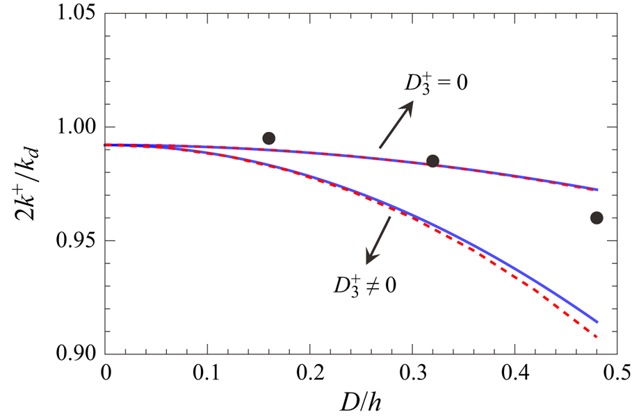
Figure 4. Comparison of wavenumber of the incident wave of the Bragg resonance among the analytical solution of (3.11) (blue solid line), the numerical results of (3.10) (red dashed line) that includes the influence of the non-resonant mode ($D_3^+ \neq 0$) or excludes this mode ($D_3^+=0$), and results of Liu et al. (2019) from the MMSE (black dots).

3.3.3. Impact of the sandbar amplitude on the magnitude of the Bragg resonance downshift

The approximate expression for the magnitude of the wave frequency downshift (3.11), which is of a parabolic form, i.e. $\delta \approx \delta _0+\delta _2$, with $\delta _0=O(1)$ and $\delta _2=O(D^2)$, reveals that with the increase of sandbar amplitude $D$, the parabolic or squared trend of $\delta$ is more pronounced than its linear trend since $\delta _1$ (the primary term of $D$ ) is always equal to zero. In addition, a threshold downshift magnitude is observed; for $D \rightarrow 0, \delta$ converges to $\delta _0$, which is negative for finite sandbar lengths $(L<\infty )$, indicating that for finite sandbar lengths, any amplitude can result in a downward shift, while for $L \rightarrow \infty$, where $\delta _0$ tends to 0, and the downshift threshold is eliminated.

To further examine the theoretical expression of the downshift magnitude and provide further insight into the phenomenon, the solutions of reflection rate and resonance frequency for gradually increased $D / h$ are presented. In case L1, the parameters $h, L, \lambda _d, N_d, k_d$, and $k$ are set to $0.22\ \mathrm {m}, 2.5\ \mathrm {m}, 0.5\ \mathrm {m}, 10,4 {\rm \pi}\ \mathrm {m}^{-1}$, and $2 {\rm \pi}\ \mathrm {m}^{-1}$. The reflection rate for various sandbar amplitudes $D$ is then calculated for a range of wave frequencies.

Figure 5(a) presents the variation of the reflection coefficients with respect to the ratio of the sandbar amplitude $D$ to the water depth $h$. The shift of the open markers indicates an enhancement of downshift behaviour of the Bragg resonance with the increase of $D / h$. Conversely, with the decrease of $D / h$, the frequency of the reflection peaks increases up to a limit of $1.1578 \ \mathrm {Hz}$, as shown in figure 5(b) (depicted by the green dotted line), with $f_{{th }}^+$ denoting the downward shift of the wave frequency to the threshold frequency. This frequency can be obtained both analytically (blue solid line from the theoretical expression (3.11)) and numerically (red dashed line, by conducting the numerical procedure for (3.10)). Overall agreement between the two solutions is observed, confirming the parabolic trend of the Bragg resonance frequency as a function of the sandbar amplitude. In addition, the wave frequency $f=\omega / 2 {\rm \pi}=1.1725 \ \mathrm {Hz}$, which is the frequency without downshift and depicted by the orange dotted line in both figure 5(a,b), is always above the other curves, indicating the downshift behaviour for any sandbar amplitude $D$. The agreement between the two solutions in figure 5(b) further demonstrates the hypothesis of the existence of a threshold frequency.

Figure 5. (a) Reflection coefficient (3.5) vs wave frequency for various $D / h$ values, with circles denoting the peak value, and the solid lines, from top to bottom, represent $D / h=0.4,0.3,0.2,0.1,0.05,0.01$. (b) Comparison of the analytical solution in (3.11) (blue solid line) and numerical results from (3.10) (red dashed line) on the frequency of the Bragg resonance vs sandbar amplitude. Green and orange dotted lines represent the threshold frequency and wave frequency, respectively.

4. Analyses of the fully nonlinear ENLS equations

In the previous work, we neglected the influence of nonlinearity on Bragg resonance for the convenience of analytical solution. However, wave nonlinearity is a key factor that affects wave transformation and reflection by altering wave speed and can cause nonlinear behaviours. In this section, the influence of nonlinearity on Bragg resonance is analysed and discussed. First, based on the Bragg resonance criteria and the nonlinear dispersion relation derived from the full nonlinear ENLS equation, we present a theoretical analysis on nonlinear Bragg scattering by the sandbars with infinitesimal amplitude. Then, the full nonlinear ENLS equation is solved numerically to investigate the wave nonlinearity impact on wave reflection by sandbars with finite amplitude.

Let $R_{{re}} (x), T_{{re}} (x)$ and $R_{{im}} (x), T_{{im}} (x)$ denote the real and imaginary parts of $R(x)$ and $T(x)$, respectively. $A^\pm$ can be expressed as

(4.1)\begin{equation} A^+=A_0 \left[T_{{re}}(x)+iT_{{im}}(x)\right] \textrm{e}^{-\textrm{i} \omega^\prime t},\quad (0< x< L) \end{equation}

and

(4.2)\begin{equation} A^-=A_0 \left[R_{{re}}(x)+iR_{{im}}(x)\right] \textrm{e}^{-\textrm{i} \omega^\prime t}.\quad (0< x< L). \end{equation}

Substituting (4.1) and (4.2) into (2.42) and (2.43), and separating real and imaginary items, we can obtain a set of nonlinear differential equations. The reflection coefficient can be obtained by:

(4.3)\begin{equation} \tilde{R}=\left|R_{{re}}(0)+\textrm{i} R_{{im}}(0)\right|. \end{equation}

4.1. Theoretical analysis on the critical $kh$ of resonance shift under infinitesimal sandbar amplitude condition

In this section, to examine the impact of wave nonlinearity on resonant wavenumber shift, the Bragg resonance criterion proposed by Mei (1985) is applied to consider a limiting condition: large number of sandbars with infinitesimal amplitude $(k_d D \rightarrow 0)$.

According to the analysis in § 3, under this condition, the following criterion, which indicates the wavenumber of the maximum reflection, can precisely predict the wavenumber of the incident wave:

(4.4)\begin{equation} k^++k^-=k_d. \end{equation}

On the side where $x<0$, waves propagate over constant water depth, and the dispersion relation for nonlinear waves can be obtained, where the wavenumbers of the incident and reflected waves can be expressed as

(4.5)\begin{equation} \left. \begin{gathered} k^+=k+\frac{\textrm{i} E_2\left(\omega^{\prime}\right)^2+\omega^{\prime}}{C_g^+}+\overbrace{A_0^2\left(\frac{\textrm{i} F_1^+}{C_g^+}+\frac{\textrm{i} F_2^+}{C_g^+} \tilde{R}^2\right)}^{\textit{wave nonlinearity induced}},\\ k^-=k+\frac{\textrm{i} E_2\left(\omega^{\prime}\right)^2+\omega^{\prime}}{C_g^+}+\underbrace{A_0^2\left(\frac{\textrm{i} F_1^+}{C_g^+} \tilde{R}^2+\frac{\textrm{i} F_2^+}{C_g^+}\right)} , \end{gathered} \right\} \end{equation}

where the third terms on the right-hand sides are the additional wavenumbers induced by the nonlinearity of incident and reflected waves, usually we have $k^+ \neq k^-$. This is a typical characteristic different from small amplitude waves condition, where the wavenumbers are identical. However, when waves approach a full reflection condition, with $\tilde {R} \rightarrow 1$, the difference induced by wave nonlinearity tends to 0 , namely $k^+-k^- \rightarrow 0$.

Combining the Bragg resonance criterion (4.4) and the dispersion relation (4.5), the non-dimensional incident wavenumber $2 k^+ / k_d$ under resonant condition can be obtained:

(4.6)\begin{equation} \frac{2 k^+}{k_d}=1+\frac{k^+-k^-}{k_d}=1+\frac{1-\tilde{R}^2}{C_g^+ k_d}\left(\textrm{i} F_1^+-\textrm{i} F_2^+\right) A_0^2, \end{equation}

where $\textrm {i} F_1^+$ and $\textrm {i} F_2^+$ are the self- and cross-modulation coefficients (Hammack et al. 2005; Onorato et al. 2006). As can be seen, for small amplitude waves $(A_0 \rightarrow 0)$, the resonance occurs at $2 k^+ / k_d=1$, as the incident wavenumber is identical to that of reflected waves. While for waves with finite wave amplitude $(A_0=O(1))$, wave self- and cross-modulation effects induce an additional shift of the resonant wavenumber, for which the shift direction is determined by $\textrm {i} F_1^+-\textrm {i} F_2^+$, whereas the former effect dominates wavenumber upshifting and the latter downshifting.

As illustrated in figure 6, the values of $\textrm {i} F_1^+$ and $\textrm {i} F_2^+$ vary with $k h$. Let $\textrm {i} F_1^+=\textrm {i} F_2^+$, combined with their definitions in (2.39), the solution for critical $k h$, which represents the condition of the prefect balance of self-modulation and cross-modulation, of resonance shift under infinitesimal sandbar amplitude condition can be obtained theoretically:

(4.7)\begin{equation} k h_0^c=1.15798 \cdots \approx 1.158. \end{equation}

Figure 6. The self-modulation $\textrm {i} F_1^+$ (black line) and cross-modulation coefficients $\textrm {i} F_2^+$ (red dashed line) vary with $k h$.

Combining the relationship presented in figure 6 and (4.6), we can find that opposing shift behaviours will occur on the two sides of $k h=k h_0^c$, owing to the discrepancy between the incident and reflected wavenumbers induced by the differences between wave self- and cross-modulation effects. More specifically, when $k h< k h_0^c$, the self-modulation effect is stronger than wave cross-modulation, resulting in $k^+>k^-$, therefore, $2 k^+ / k_d$ shifts upward with the increase of wave amplitude $A_0$. While when $k h>k h_0^c$, the cross-modulation effect becomes more pre-dominant and results in $k^+< k^-$, therefore, $2 k^+ / k_d$ shows downshift behaviour with the increase of $A_0$, where we have $k^+< k^-$.

4.2. Numerical study on critical $kh$ of resonance shift under finite sandbar amplitude condition

Under infinitesimal sandbar amplitude condition $(k_d D \rightarrow 0)$, the existence of the critical $k h$ has been theoretically demonstrated. To further consider the condition of sandbars with finite amplitude $(k_d D=O(1))$, numerical approach is needed to solve the fully nonlinear ENLS for reflection coefficient, and the details of the numerical procedure is outlined in Appendix E.

Following the set-up of experimental case D1, we set $k_d=2 {\rm \pi}\, \mathrm {m}^{-1}$ and $k={\rm \pi} \, \mathrm {m}^{-1}$, and the number of sandbars is fixed at 25. Seven cases with different sandbar amplitude $D$ were adopted, to calculate the reflection coefficients under the conditions with varying water depth, i.e. $k h=0.8 \sim 2.2$, for incident waves with different wavenumber $(2 k^+ / k_d=0.9 \sim 1.1)$ and different wave amplitude $(kA_0=0 \sim 0.08)$. The parameters of our numerical solutions are detailed in table 4, in which the calculated critical $kh$ are listed in the last columns.

Table 4. Incident wave and bottom conditions.

Figure 7 shows the reflection coefficients for three different cases, namely $k h$ is lower than, equal to and higher than the critical value $k h^c$, to illustrate the numerical procure of calculating the critical $k h$. First, we calculate the reflection coefficient under a small $k h$ condition, i.e. $k h=0.8$ for waves with different wavenumber and wave amplitude. Figure 7(a) shows that as the wave steepness increases, the wavenumber of the Bragg resonance shifts upward, in which intensifying the wave steepness significantly increases the wavenumber of the Bragg resonance. Second, the results with a large $k h$ are calculated. As shown in figure 7(c), the wavenumber of the Bragg resonance decreases monotonically with increasing wave steepness, showing a downward shift. Then, we consider the condition of a medium $k h$, i.e. $k h=(0.8+2.2) / 2=1.5$, if downshift occurs then the critical $k h$ is located between 0.8 and 1.5, otherwise we consider the region of $[1.5,2.2]$. We repeat the above procedure until we find an approximate value of $k h^c$. Specifically, for case (III), $k h=k h^c \approx 1.196$, as shown in figure 7(b), where the increase of wave nonlinearity will not induce a shift to the resonant wavenumber.

Figure 7. Comparisons of reflection coefficients vs incident wavenumber for case (III) with different $k h$ among linear analytical solution in (3.5) (blue solid line), numerical solutions for $k A_0=0$ (red dashed line), 0.06 (black dot-dashed line) and 0.08 (green dotted line): (a) $k h=0.8$; (b) $k h=1.196$; (c) $k h=2.2$.

Thus, for sandbars with finite amplitude, the critical $k h, k h^c$ still exists, which corresponds to the condition where wave nonlinearity will not induce a shift to the resonant wavenumber. Following the same calculation procedure, the relationship between $k h^c$ and $k_d D$ is obtained for cases (I)–(VII) regarding reflection coefficients for $k h$ ranging from $0.8$ to $2.2$, as illustrated in figure 8, with the critical $k h$ being the dividing line of upshift and downshift behaviour.

Figure 8. Critical $k h(k h^c)$ varies with $k_d D$.

As illustrated in figure 8, the critical $k h, k h^c$ shows an overall increase trend with the increase of sandbar amplitude. Under the condition of mild sandbar amplitude, i.e. $k_d D<0.04$, the critical $k h$ presents slight variation, and $k h^c$ tends to the critical $k h$, $k h_0^c \approx 1.158$, which has also been predicted by theoretical analysis with (4.7) as $k_d D \rightarrow 0$. For $k h< k h^c$, the frequency of Bragg resonance presents an upshift with the increase of wave nonlinearity. Whereas for $k h$ larger than $k h^c$, the regime of frequency shift induced by wave nonlinearity transits to a downshift one.

5. Conclusion

In this work, the ENLS equations have been derived by employing the multiple-scale expansion method to describe wave scattering by sinusoidal sandbars. A closed-form solution has been established by solving the linearised ENLS equations and a theoretical formula for the downshift magnitude of the resonance frequency has been proposed. The factors that influence the downshift of the Bragg resonance have been examined and the underlying mechanisms are revealed. Finally, fully nonlinear ENLS equations are solved numerically to investigate the effect of wave nonlinearity on wave reflection. The main conclusions are drawn as follows.

1. (i) Among the effects of high-order bottom, high-order dispersion and nonlinear wave–wave interaction on Bragg scattering, the high-order bottom effect is the major cause of the downshift behaviour, attributed to the combination of the re-reflection of waves and the surface modulation effect. In addition, the interaction between the forward non-resonant mode and sinusoidal sandbars also plays an important role in causing downshift behaviour, especially when the sandbar amplitude varies steeply, where a significant increase in the downward shift appears that leads to an underestimation of the downshift behaviour by the MMSE.

2. (ii) An analytical formula for the wave frequency downshift has been presented that exhibits a parabolic form with respect to the amplitude and length of sandbars, which remains valid even if the bar length approaches infinity. As the bar amplitude tends to zero, the magnitude of the frequency downshift converges to a negative threshold. This phenomenon is caused by the finite length of the sandbars and vanishes as the length approaches infinity. In addition, an expression for the wavenumber of the reflection peaks has been derived via the dispersion relation, which degenerates to the standard Bragg law as the sandbar length approaches infinity and the bar amplitude approaches zero, validating the standard Bragg law under this condition.

3. (iii) The nonlinearity of the waves has been observed to cause a shift of the Bragg resonance, with both an upward and a downward behaviour, attributed to the discrepancy between the wavenumbers of the incident and reflected waves, which is highly represented by $k h$. Under an infinitesimal sandbar amplitude condition, theoretical analysis has revealed the existence of a critical $k h, k h_0^c$, which corresponds to the condition where self-modulation equals the cross-modulation effect, where on the two sides, wave nonlinearity presents converse behaviours regarding wavenumber shift of the Bragg resonance. The self-modulation effect is responsible for wavenumber upshifting and the cross-modulation effect dominates downshifting. When $k h$ is above $k h^c$, the increase of wave nonlinearity causes a significant downshift of the Bragg resonance, where it is dominated by the cross-modulation effect with the reflected wavenumber larger than that of the incident wave. With the decreases of $k h$, the waves gradually transition from being cross-modulated-dominated to self-modulated-dominated; as a result, the incident wavenumber gradually increases and becomes larger than the reflected wavenumber, together with the gradual change of Bragg resonance frequency from downshift to upshift. Therefore, when $k h$ is smaller than the critical $k h$, the enhancement of wave nonlinearity triggers an upshift behaviour. Furthermore, numerical results have proved the relation between the critical $k h$ and sandbar amplitude $D$, which will move upwards with an increase of the amplitude of sandbars.