


1. Introduction
When a shock wave passes through a perturbed interface separating two fluids with different densities, the Richtmyer–Meshkov (RM) (Richtmyer Reference Richtmyer1960; Meshkov Reference Meshkov1969) instability occurs. The development of the RM instability is mainly driven by baroclinic vorticity produced by misalignment of the pressure and density gradients. It is hoped to be able to manipulate the RM instability, because it is a significant obstacle to the realization of inertial confinement fusion (ICF) (Lindl et al. Reference Lindl, Landen, Edwards and Moses2014). For a single-shocked interface, the perturbation amplitude will experience a linear growth, then continue to grow nonlinearly, and finally may reach a turbulent mixing stage. If the single-shocked interface experiences a second shock impact, additional vorticity will be produced. This provides a possibility to manipulate the amplitude growth rate through multiple shock impacts.
The idea that the RM instability can be manipulated through a second shock impact was first theoretically proposed by Mikaelian (Reference Mikaelian1985). If the amplitude growth rate induced by the second shock exactly cancels the growth rate caused by the first shock, the amplitude growth will stagnate, which is called ‘freeze-out’. To achieve freeze-out, the second shock should produce baroclinic vorticity of the opposite sign to that deposited by the first shock. For a heavy–light interface after the phase inversion, the second shock must propagate in the same direction as the first shock; whereas for a light–heavy interface, the second shock should propagate in the opposite direction to the first shock. By superimposing the impulsive model (Richtmyer Reference Richtmyer1960), Mikaelian (Reference Mikaelian1985) constructed a simple model to predict the time interval between the impacts of two shock waves to achieve freeze-out.
In numerical simulations, freeze-out of a heavy–light interface perturbation was realized through the impacts by two successive shock waves, i.e. two shock waves travelling in the same direction (Charakhch'yan Reference Charakhch'yan2000, Reference Charakhch'yan2001). More recently, freeze-out of a light–heavy interface perturbation was realized through a weaker reflected shock (Mikaelian Reference Mikaelian2010).
In experiments, two successive shock waves are difficult to generate in an ordinary shock tube and, therefore, experimental studies on freeze-out of a heavy–light interface perturbation are rare. A reflected shock has generally been produced through an incident shock reflecting from a rigid wall (Weber et al. Reference Weber, Haehn, Oakley, Anderson and Bonazza2012; Jacobs et al. Reference Jacobs, Krivets, Tsiklashvili and Likhachev2013; Mohaghar et al. Reference Mohaghar, Carter, Pathikonda and Ranjan2019; Guo et al. Reference Guo, Cong, Si and Luo2022). Such a reflected shock, however, is often too strong to realize freeze-out of a light–heavy perturbation. To reduce the reflected shock intensity, elastomeric foam was adopted as a ‘soft wall’ by Leinov et al. (Reference Leinov, Malamud, Elbaz, Levin, Ben-Dor, Shvarts and Sadot2009) to study the development of a light–heavy interface. Up to now, however, the experimental work on freeze-out of a light–heavy perturbation is scarce, which motivates the current work.
In this work, freeze-out of a single-mode helium–air interface accelerated by an incident shock and its reflected shock is investigated. We shall first construct a model to determine the freeze-out condition when the perturbation growth of the first-shocked interface is within the linear or weakly nonlinear stage at the arrival of the reflected shock. At the linear stage, the perturbation amplitude grows linearly, and crests and troughs of the interface develop symmetrically. At the weakly nonlinear stage, the amplitude begins to grow nonlinearly and asymmetric structures (bubble and spike) appear. However, the interface is still smooth and simply connected, and small vortices have not arisen on the spike's shoulder (Liu et al. Reference Liu, Liang, Ding, Liu and Luo2018; Zhou et al. Reference Zhou2021). To produce a weak reflected shock, a planar gas interface, instead of a rigid wall, is adopted. Then, the corresponding experiments are designed and conducted by using the initial configurations obtained from the model. It will be shown that, for both the linear and weakly nonlinear cases, freeze-out can be achieved after the reflected shock impact under the designed conditions.
2. Theoretical analysis
There are two assumptions for the theoretical analysis. First, the post-shock interface satisfies the small-perturbation hypothesis, namely,  $a_1^{-}/\lambda <0.1$, with
  $\lambda$ and
  $a_1^{-}$ being the wavelength and amplitude of the perturbation, when the reflected shock arrives. Second, the amplitude growth rates induced by the incident shock and the reflected shock follow the linear superposition principle (Mikaelian Reference Mikaelian1985), i.e.
  $v=v_{{i}}+v_{{r}}$, where
  $v$ is the amplitude growth rate after the reflected shock impact,
  $v_{{i}}$ is the growth rate induced by the incident shock just before the reflected shock impact and
  $v_{{r}}$ is the linear growth rate induced by the reflected shock. Note that
  $v_{{i}}$ here is not limited to the linear growth rate induced by the incident shock.
For the development of a single-mode light–heavy interface perturbation induced by a planar shock wave, the nonlinear model proposed by Zhang & Guo (Reference Zhang and Guo2016) (the ZG model) is adopted, since it has been widely verified to predict  $v_{{i}}$ in linear and weakly nonlinear regimes (Liu et al. Reference Liu, Liang, Ding, Liu and Luo2018; Liang et al. Reference Liang, Zhai, Ding and Luo2019; Guo et al. Reference Guo, Cong, Si and Luo2022). The ZG model can be expressed as
 \begin{equation} v_{{i}}=v_{{i}}^{{{ZG}}}(t)=\frac{1}{2}[v_{{b}}^{{{ZG}}}(t)+v_{{s}}^{{{ZG}}}(t)], \quad v_{{{b/s}}}^{{{ZG}}}(t)=\frac{v_{{i}}^{{R}}}{1+\theta kv_{{i}}^{{R}}t} , \end{equation}
where  $v_{{{b/s}}}$ is the amplitude growth rate of the bubble or spike,
  $v_{{i}}^{{R}}$ is the linear growth rate calculated by the impulsive model (Richtmyer Reference Richtmyer1960) and
 \begin{equation} \theta=\frac{3}{4}\frac{(1+A^+)(3+A^+)}{[3+A^{+}+\sqrt{2}(1+A^{+})^{1/2}]} \frac{[4(3+A^{+})+\sqrt{2}(9+A^{+})(1+A^{+})^{1/2}]} {[(3+A^{+})^2+2\sqrt{2}(3-A^{+})(1+A^{+})^{1/2}]}. \end{equation}
Here,  $A^+$ is the post-shock Atwood number, defined as
  $A^+=(\rho _2^+-\rho _1^+)/(\rho _2^++\rho _1^+)$ with
  $\rho _1^+$ and
  $\rho _2^+$ being the densities of the light and heavy fluids on both sides of the perturbed interface, after the incident shock impact. In the above,
  $v_{{i}}^{{R}}$ can be described as
 \begin{equation} v_{{i}}^{{R}}=C_1ka_0A^+\Delta u, \end{equation}
where  $a_0$ is the initial perturbation amplitude,
  $C_1$ is the incident shock compression factor (Meshkov Reference Meshkov1969) and
  $\Delta u$ is the interface velocity jump induced by the incident shock.
Through the ZG model, the perturbation amplitude just before the reflected shock impact,  $a_1^{-}=a_0C_1+\int _{0}^{\Delta t} v_{{i}}^{{{ZG}}}(t) \,{\rm {d}}t$, can be provided, in which
  $\Delta t$ is the time interval between the impacts of two shock waves. Specifically, if the amplitude growth is within the linear stage when the reflected shock arrives,
  $v_{{i}}$ can be directly predicted by the impulsive model, i.e.
  $v_{{i}}=v_{{i}}^{{R}}$. In this work, to ensure the validity of the ZG model, only the linear and weakly nonlinear stages of the amplitude growth are involved.
When the reflected shock impacts the evolving heavy–light interface, rarefaction waves are reflected. The irrotational model proposed by Wouchuk & Nishihara (Reference Wouchuk and Nishihara1997) (the WN model) has been verified to accurately predict the linear growth rate of a shocked single-mode interface when a rarefaction wave is reflected (Wouchuk Reference Wouchuk2001). In the present work, the linear growth rate induced by the reflected shock  $v_{{r}}$ can be predicted by the WN model as
 \begin{equation} v_{{r}}=ka_1^{-}f(M_{{s}1}, M_{{s}2}, \rho_{1}, \rho_{2}, \gamma_{1}, \gamma_{2}). \end{equation}
Here,  $\rho _{1}$ and
  $\rho _{2}$ (
 $\gamma _{1}$ and
  $\gamma _{2}$) are the initial densities (specific heat ratios) of the light and heavy fluids on both sides of the perturbed interface, while
  $M_{{s}1}$ and
  $M_{{s}2}$ are the Mach numbers of the incident shock and reflected shock when they encounter the interface. The function
  $f$ can be expressed as
 \begin{equation} f=\frac{\rho_{1{{r}}}\Delta u_{{r}}\left(1-\dfrac{V_{{{rt}}}}{V_{{{rs}}}}\right)+ \rho_{2{{r}}}(\Delta u_{2{{r}}} -\Delta u_{{r}})\left(1+\dfrac{V_{{{rf}}}}{V_{{{rs}}}}\right)} {\rho_{1{{r}}}+\rho_{2{{r}}}}. \end{equation}
Here,  $\rho _{1{{r}}}$ and
  $\rho _{2{{r}}}$ are the densities of the light and heavy fluids on both sides of the interface after the reflected shock impact;
  $V_{{{rs}}}$,
  $V_{{{rf}}}$ and
  $V_{{{rt}}}$ are the velocities of the reflected shock, the rarefaction wave front and the re-transmitted shock, respectively; and
  $\Delta u_{{r}}$ and
  $\Delta u_{2{{r}}}$ are the interface velocity jumps induced by the reflected shock and the heavy fluid velocity after the reflected shock impact. These parameters in (2.5) can be solved using one-dimensional (1-D) gas dynamics theory by providing shock Mach numbers and initial parameters.
According to the analysis above,  $v$ can be theoretically predicted if the initial parameters are provided. When
  $v=0$, the interface amplitude remains constant after the reflected shock impact, i.e. the amplitude growth is ‘frozen out’. The relationship among the initial parameters can be determined to realize freeze-out by using (2.1a,b) to (2.5). In particular, if
  $v_{{i}}$ belongs to the linear growth rate regime, the freeze-out condition is independent of
  $a_0$. When the shock intensities and the properties of the gases on both sides of the interface are fixed, to realize freeze-out, the initial perturbation wavelength (
 $\lambda$) and
  $\Delta t$ satisfy a linear relationship:
 \begin{equation} \Delta t/\lambda={-}(\,f+A^+\Delta u)/(2{\rm \pi} fA^+\Delta u). \end{equation}
This relationship in the ( $\lambda, \Delta t$) plane is called the freeze-out line. However, if the amplitude grows nonlinearly at the arrival of the reflected shock, the freeze-out condition is also dependent upon
  $a_0$, and such a linear relationship between
  $\lambda$ and
  $\Delta t$ does not exist.
3. Experimental method
Experiments are performed to achieve freeze-out under the proper conditions determined by the model. To produce a weak reflected shock, a planar air–SF $_6$ (sulfur hexafluoride) or air–argon interface, instead of a rigid wall, is adopted. Selection of either SF
 $_6$ or argon is dependent on the reflected shock strength. If the amplitude growth is linear (weakly nonlinear) when the reflected shock arrives, an air–SF
 $_6$ (air–argon) interface is adopted to generate a relatively strong (weak) reflected shock. The intensities of the reflected shock waves when using these different gas combinations are listed in table 1.
Table 1. Parameters in all cases:  $L_0$ is the distance from the average position of the single-mode helium–air interface to the planar air–SF
 $_6$ (air–argon) interface;
  $a_0$ is the initial amplitude and
  $a_1^-$ is the amplitude just before the reflected shock arrival;
  $\lambda$ is the perturbation wavelength;
  $M_{{s}1}$ and
  $M_{{s}2}$ are the Mach numbers of the incident shock and reflected shock;
  $\varphi ({\rm He})$ is the helium volume fraction in space A;
  $A^+$ is the post-shock Atwood number;
  $\Delta t$ is the time interval between the impacts of two shock waves; and
  $\Delta u$ and
  $\Delta u_{{r}}$ are the helium–air interface velocity jumps induced by the incident shock and reflected shock. The superscripts ‘t’ and ‘e’ denote theoretical and experimental results. The units for length, velocity and time are mm,
  ${\rm m}~{\rm s}^{-1}$ and
  $\mathrm {\mu }{\rm s}$, respectively.

The soap film technique (Liu et al. Reference Liu, Liang, Ding, Liu and Luo2018; Liang et al. Reference Liang, Zhai, Ding and Luo2019) is adopted to create the interfaces. As shown in figures 1(a) and 1(b), there are three interfaces, including a perturbed one and two undisturbed ones. The first interface AI $_1$ (undisturbed) is used to separate helium (in space A) from air in the driven section; the second interface II (perturbed) to separate air (in space B) from helium (in space A) to create a single-mode helium–air interface; and the third interface AI
 $_2$ (undisturbed) to separate SF
 $_6$ or argon (in space C) from air (in space B) for reflecting a weak shock. To generate the interfaces separating the different gases, after the soap film interfaces are formed at the preset positions, light gas (helium) and heavy gas (SF
 $_6$ or argon) are pumped into spaces A and C, respectively, through the inflow holes, and air is slowly discharged through the outflow holes.

Figure 1. Schematics of the soap film interface generation (a) and the initial configuration studied (b). Here, AI $_1$ and AI
 $_2$ are two undisturbed auxiliary interfaces; II is the initial helium–air interface; SW
 $_1$ is the incident shock; and
  $L_0$ is the initial distance between II and AI
 $_2$.
$_2$.
For all experimental runs, the inflation rate and duration are the same to ensure similar volume fractions of light and heavy gases in the spaces as far as possible. Because helium is easily polluted, the contamination of helium by air in space A is considered, whereas the gases in the other spaces are considered as pure. The helium concentration is determined by comparing the measured velocities of the incident shock, the transmitted shock and the helium–air interface velocity jump in experiments with those predicted from 1-D gas dynamics theory. The distance between II and AI $_1$ is 100 mm, which is large enough to ensure that the interface-coupling effect and the disturbance waves will not affect the development of the helium–air perturbation (Liang & Luo Reference Liang and Luo2021). The distance between II and AI
 $_2$ is defined as
  $L_0$, which is flexible to change the time interval
  $\Delta t$.
The experiments are conducted in a horizontal shock tube (Guo et al. Reference Guo, Cong, Si and Luo2022), and the Mach number of the incident plane shock moving in helium is  $1.19\pm 0.01$. The post-shock flow field is recorded by high-speed schlieren photography. The frame rate of the camera (FASTCAM SA5, Photron Ltd) is 50 000 frames per second and the exposure time is
  $1~\mathrm {\mu }{\rm s}$. Owing to the different sizes of the observation domains required, the spatial resolution ranges from 0.38 to
  $0.45~{\rm mm}~{\rm pixel}^{-1}$. The ambient pressure and temperature are
  $101.3\pm 0.1$ kPa and
  $295\pm 1.5$ K, respectively. We note that, due to the limitation of the observation window, the developments of these three interfaces cannot be captured simultaneously by the camera. Since the emphasis is on the development of the single-mode interface, in the following experiments, both helium–air and air–SF
 $_6$ (or air–argon) interfaces (II and AI
 $_2$) are shown in the schlieren images, whereas the air–helium interface (AI
 $_1$) is absent.
4. Results and discussion
4.1. Unperturbed case
In experiments, we first verify that AI $_1$ will not affect the development of II. For this purpose, the movements of AI
 $_1$ and the undisturbed II after shock impact are studied, and the corresponding schlieren images are presented in figure 2(a). The initial time is defined as the moment when the incident shock (SW
 $_1$) meets the interface, and similarly hereinafter. As SW
 $_1$ impinges on II, a transmitted shock wave (
 ${\rm SW}_1^{{t}}$) and a once-shocked helium–air interface (OSI) are formed. During the time studied, the shocked AI
 $_1$ (SAI) is always far away from the OSI. Note that SAI is deformed slightly after it passes across the holes (
 $307~\mathrm {\mu }{\rm s}$). Later, the small disturbances on SAI develop significantly (
 $747~\mathrm {\mu }{\rm s}$), which is primarily caused by the filaments used to restrict the soap film interface. However, the disturbances on the OSI can still be ignored, which is consistent with the previous work in helium layers (Liang & Luo Reference Liang and Luo2021). Therefore, the interface-coupling effect is negligible.

Figure 2. Evolution of a plane helium–air interface induced by a plane shock (a) and the trajectories of the interface and the shock waves (b). Here,  $\Delta L$ is the distance of the evolving interface from the initial position of II; OSI is the once-shocked interface; SAI is the shocked auxiliary interface; and
  ${\rm SW}_1^{{t}}$ is the first transmitted shock. Other symbols have the same meaning as those in figure 1.
The trajectories of the shock waves and OSI extracted from the schlieren images are shown in figure 2(b). Both the shock waves and OSI move linearly, which means that the OSI has not been affected significantly by additional waves except SW $_1$. Through measuring the velocities of the shock waves and OSI, and combining with 1-D gas dynamics theory, the volume fraction of helium in space A is calculated to be
  $68\,\%\pm 5\,\%$ from multiple experimental runs. Note that the helium concentration influences both the shock intensity and the amplitude growth and, therefore, affects the prediction of the freeze-out condition. In experiments, however, it is almost impossible to precisely control the helium concentration because helium has a much smaller molecular weight and diffuses much faster.
In the following studies, seven kinds of single-mode helium–air interface with different  $\lambda$ and
  $a_0$, as shown in table 1, are considered. For each case, according to the range of helium concentration in the undisturbed case, the freeze-out conditions of the single-mode helium–air interfaces with different initial conditions are predicted theoretically. Then multiple experimental runs are conducted until the experimental parameters satisfy the freeze-out condition. The parameters in each case in table 1 satisfy the small-perturbation hypothesis and the freeze-out condition. Specifically, the initial parameters in the former four cases (latter three cases) ensure the linear (weakly nonlinear) growth of the perturbation at the arrival of the reflected shock. Note that different initial conditions in weakly nonlinear cases from those in linear cases are selected, mainly because the perturbation with a larger wavelength needs more time to achieve freeze-out in weakly nonlinear cases. However, due to the limitation of the test section length, the time interval
  $\Delta t$ cannot be regulated over a wide range in this work.
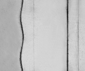
4.2. The linear cases
In this subsection, we consider the linear case, i.e. the perturbation growth of the shocked interface is in the linear stage at the arrival of the reflected shock. Specifically, four single-mode helium–air interfaces with almost the same  $a_0/\lambda$ but different
  $\lambda$ are studied (cases 1–4 in table 1). An air–SF
 $_6$ plane interface is adopted here to produce the reflected shock. The typical schlieren images of the helium–air interfaces accelerated by the incident shock and the reflected shock are provided in figure 3. Note that the shocked AI
 $_1$ is not shown in the images because it does not affect the perturbed interface evolution.

Figure 3. Typical schlieren images showing the interface evolution and wave patterns for cases 1–4. Here,  ${\rm SW}_2^{{r}}$ is the shock of
  ${\rm SW}_1^{{t}}$ reflected from AI
 $_2$;
$_2$;  ${\rm SW}_2^{{t}}$ is the shock of
  ${\rm SW}_1^{{t}}$ transmitted from AI
 $_2$; SAI
 $_2$ is the shocked AI
 $_2$; and DSI is the double-shocked interface. The contrast was enhanced without loss of trust.
Taking case 1 as an example, when SW $_1$ interacts with II, a transmitted shock (
 ${\rm SW}_1^{{t}}$) and a reflected shock are generated (
 $69~\mathrm {\mu }{\rm s}$). This reflected shock moving in helium is invisible due to its weak intensity. The shocked II (OSI) starts to move downstream with its amplitude increasing. Because the amplitude of II is small,
  ${\rm SW}_1^{{t}}$ quickly recovers to a planar shock. Subsequently,
  ${\rm SW}_1^{{t}}$ impacts AI
 $_2$, generating a transmitted shock (
 ${\rm SW}_2^{{t}}$) and a reflected weak shock (
 ${\rm SW}_2^{{r}}$) (
 $389~\mathrm {\mu }{\rm s}$). Before
  ${\rm SW}_2^{{r}}$ impact, the amplitude of the OSI grows continuously. After
  ${\rm SW}_2^{{r}}$ collides with the OSI, the amplitude almost stops growing (
 $469\unicode{x2013}669~\mathrm {\mu }{\rm s}$). In other words, the growth rate induced by SW
 $_1$ is eliminated completely by the reflected shock, and the amplitude growth is frozen out.
The variations of the dimensionless amplitudes in the different cases before and after the reflected shock impact are shown in figure 4(a). The time is normalized as  $\tau =kv_{{i}}^{{e}}(t-t^*)$, where
  $v_{{i}}^{{e}}$ is the linear growth rate of the OSI in experiments and
  $t^*$ is the time when the linear growth of the OSI amplitude starts (generally compression phase ends). The amplitude is scaled as
  $\alpha =k(a-a^*)$, where
  $a^*$ is the perturbation amplitude at
  $t=t^*$, which differs from the initial amplitude. From figure 4(a), the amplitudes of the OSI grow linearly before
  ${\rm SW}_2^{{r}}$ arrives. The linear growth rates of the OSI measured from the experiments and predicted from the impulsive model (Richtmyer Reference Richtmyer1960) are compared in table 2, and a good agreement is reached. After
  ${\rm SW}_2^{{r}}$ impacts the OSI, the amplitude rises again before it settles in the steady-state value in cases 1–3. Such a phenomenon, however, is absent in case 4. Note that the amplitude growth induced by the reflected shock needs a start-up process (Lombardini & Pullin Reference Lombardini and Pullin2009). In cases 1–3, it is probable that the start-up process has not ended when the compression process ends, and the start-up process results in the rise of amplitude growth. In case 4, the wavelength is relatively smaller, and the start-up process is relatively shorter (Lombardini & Pullin Reference Lombardini and Pullin2009). The absence of the ascent process of amplitude growth is probably ascribed to the longer compression process than the start-up process. Besides, the limited temporal resolution in experiments may also cause this disparity. Although the amplitudes of these four cases are different, their growths are almost stagnated. As a result, freeze-out of amplitude growth of a single-mode helium–air interface is realized through a weak reflected shock in shock-tube experiments.

Figure 4. (a) Temporal variations of the dimensionless perturbation amplitude in cases 1–4. The solid line stands for the prediction from the impulsive model. (b) Freeze-out lines and distribution of initial parameters of different cases in the  $\lambda$–
 $\Delta t$ plane. Here, freeze-out lines 1, 2 and 3 correspond to cases 1 and 2, cases 3 and 4, and cases 5 to 7, respectively.
Table 2. Comparison of the linear growth rates of the OSI between experiments and predictions from the impulsive model.

As indicated in § 2, if the perturbation growth is within the linear regime at the arrival of the reflected shock,  $\lambda$ and
  $\Delta t$ satisfy a linear relationship. To verify this relation, the ‘freeze-out lines’ calculated by (2.6) are provided in figure 4(b). Note that the helium concentrations in cases 1 and 2 are different from those in cases 3 and 4; thus the freeze-out lines are therefore different, as indicated by freeze-out line 1 and freeze-out line 2, respectively. The experimental parameters are well located at the freeze-out lines, which experimentally verifies the linear relationship between
  $\lambda$ and
  $\Delta t$. For each case, actually, more than two experimental runs are performed. We find that when freeze-out is achieved, the difference of
  $\Delta t$ among cases is within
  $5~\mathrm {\mu }{\rm s}$. According to this linear relationship, the initial parameters can be easily controlled to realize freeze-out.
4.3. The weakly nonlinear cases
In this subsection, the weakly nonlinear growth of the perturbation at the arrival of the reflected shock is considered. Three single-mode helium–air interfaces with the same small  $\lambda$ but different
  $a_0$ are tested (cases 5–7 in table 1). Because the growth rate in the weakly nonlinear regime is smaller than that in the linear regime, to offset the smaller growth rate, an even weaker reflected shock is needed. As a result, an air–argon interface, instead of an air–SF
 $_6$ interface, is adopted here to produce a weaker reflected shock. The weak reflected shock results in a longer
  $\Delta t$ for the same
  $L_0$. A longer
  $\Delta t$ and a smaller
  $\lambda$ allow the amplitude to grow more quickly into the weakly nonlinear regime.
Figure 5 shows the evolutions of the single-mode helium–air interfaces accelerated by the incident shock and the reflected shock in cases 5–7. The wave patterns are quite similar to cases 1–4, and, therefore, the description is omitted. Taking case 7 as an example, before  ${\rm SW}_2^{{r}}$ arrives (
 $253~\mathrm {\mu }{\rm s}$), the slightly asymmetric developments of the crest and trough occur, indicating the weakly nonlinear growth of the perturbation. After
  ${\rm SW}_2^{{r}}$ passes through the OSI (
 $333~\mathrm {\mu }{\rm s}$), the amplitude of the DSI remains almost constant. However, the interface profile changes with time, which is caused by the generation of the second-order harmonic (Liu et al. Reference Liu, Liang, Ding, Liu and Luo2018). This will be discussed in the following paragraph.

Figure 5. Typical schlieren images showing the interface evolution and wave patterns for cases 5–7.
Temporal variations of the dimensionless amplitude for cases 5–7 before and after  ${\rm SW}_2^{{r}}$ impact are plotted in figure 6(a). Indeed, the perturbation growth enters the weakly nonlinear regime at the arrival of
  ${\rm SW}_2^{{r}}$. The prediction from the ZG model is also included, and agrees well with the experimental results. As a result, the amplitude and growth rate of the OSI when the reflected shock arrives can be calculated by the ZG model (2.1a,b). After
  ${\rm SW}_2^{{r}}$ impinges upon the OSI, the ascent process of the amplitude growth is absent. In weakly nonlinear cases, the reflected shock is weaker and the amplitude is larger when the reflected shock arrives relative to linear cases. A relatively longer compression process may result in the absence of the ascent process, as explained in § 4.2. For cases 5–7, the amplitude growth almost stagnates, and freeze-out is realized. The
  $\Delta t$ for achieving freeze-out predicted from the model for cases 5–7 are 435, 357 and
  $305~\mathrm {\mu }{\rm s}$, respectively, which are in good agreement with the experimental counterparts, as given in table 1. This fact shows that, even if the perturbation growth is within the weakly nonlinear regime, freeze-out can still be achieved and predicted.

Figure 6. Temporal variations of the dimensionless amplitude before and after the reflected shock impact for the cases 5–7 (a) and amplitude developments for the first three harmonics (b).
It is worth noting that when the OSI growth is weakly nonlinear, in order to realize freeze-out,  $\Delta t$ is related not only to
  $\lambda$ but also to
  $a_0$. Therefore, a single freeze-out line does not exist. In figure 4, the freeze-out line 3 is calculated based on the initial parameters of
  $\varphi ({\rm He})=70\,\%$,
  $M_{{s}1}=1.19$ and
  $M_{{s}2}=1.02$. It is found that the
  $\Delta t$ for cases 5–7 cannot be predicted by the linear relation (2.6), and, as the initial amplitude increases, the measured
  $\Delta t$ deviates more from the freeze-out line. Figure 6(b) shows the amplitude growths of the first three harmonics. The amplitude of the fundamental mode is almost equal to the overall amplitude of the perturbation, and can be well predicted by the ZG model before the reflected shock impact. After the reflected shock impact, the amplitude growth of the fundamental mode nearly stagnates, but the amplitude of the second-order harmonic continues to grow, changing the interface profile. However, the second-order harmonic does not change the interface amplitude in the linear and weakly nonlinear stages (Guo et al. Reference Guo, Cong, Si and Luo2022), and thus will not affect the realization of freeze-out.
5. Conclusions
Freeze-out of amplitude growth of a shocked single-mode helium–air perturbation is realized through a weak reflected shock both theoretically and experimentally. Theoretically, two cases are considered. First, if the perturbation growth is within the linear regime when the reflected shock arrives (denoted as the linear cases), the impulsive model (Richtmyer Reference Richtmyer1960) and the linear model (Wouchuk & Nishihara Reference Wouchuk and Nishihara1997) are combined to calculate the relation among the initial parameters. It is found that the time interval  $\Delta t$ between the impacts of two shock waves is linearly related to the perturbation wavelength
  $\lambda$ for achieving freeze-out, and is independent of the initial amplitude
  $a_0$. Second, if the perturbation growth is within the weakly nonlinear regime at the arrival of the reflected shock (denoted as the nonlinear cases), the nonlinear model (Zhang & Guo Reference Zhang and Guo2016) and the linear model (Wouchuk & Nishihara Reference Wouchuk and Nishihara1997) are adopted. It is found that
  $\Delta t$ is related to both
  $\lambda$ and
  $a_0$.
Experimentally, a light–heavy plane interface, instead of a rigid wall, is adopted to produce the weak reflected shock. The soap film technique is used to create the initially perturbed and undisturbed interfaces, and high-speed schlieren photography is used to capture the post-shock flow. Seven experimental runs, including four linear cases and three nonlinear cases, are considered. For the linear cases, the amplitude stops growing after the reflected shock impact, and the linear relationship between  $\Delta t$ and
  $\lambda$ is verified experimentally. For the nonlinear cases, freeze-out can still be realized through a weaker reflected shock, but the linear relationship between
  $\Delta t$ and
  $\lambda$ does not exist. As a whole, a single-mode light–heavy perturbation can achieve amplitude freeze-out through a reflected shock. These findings may be helpful for better understanding how to suppress hydrodynamics instabilities in ICF. Note that only limited observations of this phenomenon are presented in the current work. More cases with a wider range of conditions will be tested in following work. Besides, the amplitude manipulation of a heavy–light interface subjected to a shock will also be investigated because in ICF the initial shock propagates from a heavy fluid to a light one.
Funding
This work was supported by the National Natural Science Foundation of China (nos. 12022201, 91952205 and 12102425) and Youth Innovation Promotion Association CAS.
Declaration of interests
The authors report no conflict of interest.


