Hydrodynamic metamaterial redirector for steering fluid flow in pipelines with arbitrary curvatures

Abstract

The dynamics of fluid-conveying pipelines with different shapes has received extensive research attention. Significant wall shear stress and flow separation occur when the fluid flows through pipelines with various curvatures. These phenomena trigger pipeline vibration, the generation of mechanical and hydrodynamic noise, damage, and even the rupture of the pipeline. However, previous studies have not considered the mechanism of internal pipeline flow to eliminate flow separation and the generation of secondary flow inside bent pipelines by redirecting and manipulating the flow. To steer the fluid flow, a ‘hydrodynamic transformation strategy’ based on the metamaterial technology is proposed for the first time in this work; through this strategy, the fluid in pipelines can be made to flow along trajectories that are always parallel to the central axis of the bent pipelines. Interestingly, this innovative method can effectively eliminate the elbow-induced secondary flow and prevent the generation of a pressure gradient toward the pipeline wall. Using the soft lithography technology or the three-dimensional printing technology, the hydrodynamic metamaterial microstructure required to manipulate the fluid flow path in actual engineering applications can be achieved. Our work paves the way for developing new approaches for controlling the flow characteristics and reducing the turbulence intensity of the fluid flowing in pipelines with elbows and corners.

1. Introduction

Fluid-conveying pipelines are an essential component of substance transportation and cooling systems, and are thus widely used in many fields, such as naval and ocean engineering (Wiggert & Tijsseling 2001; Łuczko & Czerwiński 2019; Beauvais et al. 2021; Zheng et al. 2021; Zhang et al. 2023), high-performance data centres (Zhang et al. 2022; Chen et al. 2023; He et al. 2023; Xue, Ai & Qu 2023), biological vessels (McCarthy & Smith 2002; Liao 2012; Leslie et al. 2014) and even microfluidic chips (Pattanayak et al. 2021; Chen et al. 2022; Fang et al. 2022), as shown in figure 1. When passing through the elbow of pipelines, the fluid is subjected to resistance as well as secondary backflow due to the changes in the curvature of the pipelines, which could result in major safety accidents. To obey the conservation of mass law and since it is affected by the elbow-induced resistance, the fluid has no choice but to bend toward the inside wall, generating flow separation, secondary flow and vortex-induced vibrations inside the pipelines, and these phenomena affect the entire flow field (Finlay, Keller & Ferziger 1988). In addition, altered haemodynamics result in changes in the shear forces generated by the blood against the wall. These flows can adversely affect the intima of the blood vessels, causing damage to the endothelium and the formation of thrombi or aneurysms (Virani et al. 2021). Therefore, it is vital to prevent the formation of irregular flow patterns inside pipelines in various application fields.

Figure 1. Schematic of possible application scenarios of fluid-conveying pipelines and conceptual design of hydrodynamic metamaterials.

Conventionally, in the hydraulic and cooling systems of underwater vehicles, the most widely used methods to reduce unstable internal flow to avoid the resonance issue caused by the curvature variation of the fluid-conveying pipeline are: (1) parametrically optimize the layout of elastic supports to shift the natural frequency of the pipeline away from the excitation frequency (Cao, Liu & Hu 2023; Yang, Qin & Zhang 2023; Zhang et al. 2023); (2) use composite pipelines with a high specific stiffness, a high fatigue resistance, better buffering and vibration damping properties (Li et al. 2021; Wiggert & Tijsseling 2001; Wu et al. 2023); (3) adopt the casing approach, i.e. wrap the fluid-conveying pipeline in an outside pipeline layer and fill the interval between the two with cushioning and vibration-damping materials, such as fibres (Mehmood et al. 2020; Guo et al. 2022). However, these methods do not consider the fluid flow mechanism within the pipeline, and it remains fundamentally impossible to eliminate the instability of the internal flow field.

In the modern information and digital era, while we enjoy the convenience brought by big data analysis, cloud services, high-performance parallel computing and artificial intelligence, we need to address the related increase in energy consumption and comply with stricter thermal management requirements of data centres (Dang, Jia & Lu 2017). Data centres consume up to 416 billion kWh of electricity each year, which accounts for almost 2.0 % of the global electricity, and thus represent a significant proportion of global power consumption (Sulaiman, Daraghmeh & Wang 2020; Ding et al. 2022). Surprisingly, up to 40 % of the electricity is used for mechanical-vapor-compression cooling systems for the data hosts (Dayarathna, Wen & Fan 2016). Moreover, with the rapid development of high-performance central processing units as well as graphics processing units, future cooling systems will have to face an even greater challenge. With the low cooling and heat dissipation efficiency of traditional room-level air-conditioning systems, as well as the requirements of reducing energy consumption and greenhouse gas emissions, the water-cooling technology stands out due to the high specific heat of water. In addition, owing to its low greenhouse gas emissions and low failure rate, the water-cooling technology is favoured by many IT companies and organizations (Lamb 2009). However, water-cooling pipeline systems must be embedded within high-energy-consumption areas, such as central processing units. Once fatigue damage or rupture of the pipeline occurs during its service cycle, server failure may be triggered, which may even lead to the paralysis of the entire city network; thus, the reliability and safety of water-cooling pipeline systems are critical.

Our fast-paced modern lifestyle is stressful for many individuals. Staying up late, alcoholism, smoking, obesity and other bad habits have increasingly become strategies for people to release stress, which leads to the risk of developing cardiovascular disease increasing year by year (Murphy et al. 2021). Fortunately, with the rapid advancements in the modern medical technology, the design of artificial tissue organs and vascular stents has reduced the number of patients suffering with cardio-cerebrovascular diseases (CCVDs) (Oxley et al. 2016; Opie et al. 2018). However, the biocompatibility between medical devices implanted in vitro and blood needs to be further improved. Surface-induced thrombosis has become a notorious issue of medical devices that come in contact with blood, which poses a severe threat to the safety of patients and potentially undermines the proper function of the equipment, especially in irregular vessels, such as bifurcated and curved vessels, where the chances of thrombus formation are greater (Gori et al. 2019). Typically, artificial tissues, organs and vascular stents are implanted alongside considerable drug elution (including fixing anticoagulants, changing the surface chemistry and morphology, and releasing antithrombotic compounds). More worryingly, the long-term use of anticoagulant drugs for delaying secondary thrombus formation can easily lead to haemolysis and other complications (Wouk et al. 2021). To alleviate the suffering of patients with CCVDs, bypass the need for systemic anticoagulation and reduce drug intake, researchers have started to study the haemodynamic mechanism. Antithrombotic microstructure materials, such as biomimetic hydrophobic coatings, have been proposed to improve the flow pattern of curved blood vessels (Sharma et al. 2018; Jinnouchi et al. 2019). Therefore, the design of new microstructured implant materials based on the fluid dynamics theory has promising applications for improving the experience of patients with CCVDs and prevent secondary diseases.

As the core of microfluidic chips, microfluidic devices have been used to construct microfluidic control modules with their microstructure, symmetric and asymmetric column arrays (Hughes et al. 2012; Cui & Wang 2019). Microfluidic devices provide new strategies for controlling the microfluidic flow path and enable novel microbial screening analyses, representing a promising tool for drug development and applied research. Microfluidic chips have become a research hotspot owing to their capacity for efficient flow control, high sensitivity and advanced analytical performance, and have been widely used in a broad range of fields, such as chemical synthesis (Elvira et al. 2013), proteomics (Hughes et al. 2012), single-cell analysis (Yang, Giessen & Lalanne 2015) and peristalsis of human colon tumour organoids on microfluidic chips (Fang et al. 2022). In addition, due to their excellent biocompatibility, superior electrical insulation and heat dissipation, excellent optical properties, and simple and low-cost production processes, microfluidic devices are becoming a powerful tool for clinical drug development, rapid screening and clinical analysis (Rembert et al. 2023).

Recently, metamaterials have attracted enormous attention in the scientific community as it has been reported that they can be used to manipulate physical fields (Leonhardt 2006; Pendry, Schurig & Smith 2006; Schittny et al. 2013; Martinez & Maldovan 2022). The foundation of metamaterial design and space warping originates from Einstein's general theory of relativity, where it is assumed that gravity can warp both space and time through the action of force fields (Albert, Perrett & Jeffery 1916). The manipulation of various physical fields is an innovative concept in material design that has become feasible through the use of metamaterials; at the same time, a revolution in the optics research field has occurred (Cai et al. 2007; Chen, Chan & Sheng 2010; Xu & Chen 2014). Subsequently, inspired by the theoretical framework of transformation optics, several interdisciplinary research fields have emerged, such as transformation acoustics, transformation thermodynamics and transformation electromagnetism.

It is well known that spatial coordinate transformations offer a unique way to redirect the physical field by transforming constant physical properties into inhomogeneous and anisotropic properties. Typically, transformation optics can be used to manipulate the propagation path of light by first transforming the permittivity and permeability of the medium into an anisotropic tensor, and then designing an equivalent metamaterial structure characterized by that anisotropic tensor (Chen & Chan 2008; Jiang et al. 2008). Similar to the manipulation of physical fields achieved in transformation optics, the physical properties required for manipulating the flow field in fluid mechanics, i.e. fluid density $\rho $ and dynamic viscosity $\mu $, can be determined by designing corresponding hydrodynamic metamaterials (Morton et al. 2008; Urzhumov & Smith 2011; Park, Youn & Song 2019; Pang et al. 2022). However, metamaterials capable of redirecting fluid in flow-conveying pipelines with arbitrary curvature have not yet been developed.

In this work, an innovative strategy is proposed to steer and redirect the internal flow field of fluid-conveying pipelines with arbitrary curvatures to eliminate unsteady flow phenomena, such as flow separation and irregular secondary flow. This strategy harnesses a spatial coordinate transformation to establish a spatial mapping relationship between pipelines with arbitrary curvatures and straight pipelines. Hydrodynamic metamaterial steering devices for fluid-conveying pipelines are thus obtained, which permit the establishment of a steady flow state. Our work opens up new possibilities for manipulating the internal flow of fluid-conveying pipelines, and could stimulate the development of related drag-reduction and energy-saving technologies.

2. Problem formulation and theory

Due to the constraints in the spatial layout imposed by different application scenarios, pipelines with arbitrary curvatures, cross-sections and bending forms are often indispensable. However, changes in the shape and curvature of pipelines can lead to secondary flow and an increase in turbulence intensity, threatening the safety of the pipeline as well as the entire equipment. Therefore, suppressing and eliminating elbow-induced flow separation and secondary flow has become an objective of research in various fields.

2.1. Establishment of the spatial transformation theory

To eliminate the resistance sources and prolong the service life of pipelines, a strategic flow redirector for arbitrarily bent pipelines based on the utilization of the Navier−Stokes equations is developed. In pioneering works on transformation hydrodynamics, several reports have reported different transformed densities $\rho $ and dynamic viscosities $\mu $ for designing hydrodynamic cloaks (Urzhumov & Smith 2011; Park et al. 2019; Pang et al. 2022). Although there exist several approaches for obtaining anisotropic physical parameters based on different spatial transformation backgrounds, the main concept is to transform the Navier−Stokes equations in different coordinate spaces to obtain the anisotropic micro–nano metamaterial parameters required for manipulating fluid trajectories.

Being a second-order, strongly nonlinear, partial differential equation system, the Navier−Stokes equations have been used to address numerous open problems related to viscous flow in the scientific and engineering communities. It is well known that the most important properties of a fluid are its density $\rho $ and viscosity $\mu $, which determine the compressibility and viscous resistance of the fluid, respectively. Naturally, they also dramatically affect the forces acting on an object immersed in the fluid. Based on these premises, the Navier−Stokes equations are here employed without considering the source term force. Thus, the integral form of the Navier−Stokes equations is

(2.1) \begin{equation}\left. {\begin{gathered} {\dfrac{\partial }{{\partial t}}\int_V {\rho \boldsymbol{V}\,\textrm{d}V} + \int_{\partial V} {\rho \boldsymbol{VV}\,\textrm{d}\boldsymbol{S}} = \int_{\partial V} {\bar{\boldsymbol{\bar{\tau }}}\,\textrm{d}\boldsymbol{S}} - \int_{\partial V} {p\,\textrm{d}\boldsymbol{S}} ,}\\ {\dfrac{\partial }{{\partial t}}\int_V {\rho \,\textrm{d}V} + \int_{\partial V} {\rho \boldsymbol{V}\,\textrm{d}\boldsymbol{S}} = 0,} \end{gathered}} \right\}\end{equation}

where $\boldsymbol{V}$ is the velocity vector, $\textrm{p}$ is the static pressure, $\bar{\boldsymbol{\bar{\tau }}}$ is the viscous stress tensor, t is the time and S is the surface enclosed by the control volume V. For a fluid, the developed viscous stress loads are directly proportional to the element strain rates and the dynamic viscosity coefficient. In the natural state, the dynamic viscosity of the fluid is regarded as a constant.

To be able to manipulate the fluid flow in a fluid-conveying pipeline, while keeping the form invariant of the Navier−Stokes equations before and after the coordinate transformation, the binary product of the velocity vector $\boldsymbol{V}$ with itself is treated here as a tensor (as shown in (2.2)). This treatment simplifies the establishment of the redirection theory and facilitates the efficient utilization of the traditional algorithms for solving the Navier−Stokes equations.

(2.2) \begin{equation}\begin{aligned} \bar{\boldsymbol{\bar{G}}} & = \rho \{ \boldsymbol{VV}\} = \rho (u\boldsymbol{i} + v\boldsymbol{j} + w\boldsymbol{k})(u\boldsymbol{i} + v\boldsymbol{j} + w\boldsymbol{k})\\ & = \rho (uu\boldsymbol{ii} + uv\boldsymbol{ij} + uw\boldsymbol{ik} + vu\boldsymbol{ji} + vv\boldsymbol{jj} + vw\boldsymbol{jk}\\ & \quad + wu\boldsymbol{ki} + wv\boldsymbol{kj} + ww\boldsymbol{kk})\\ & = \rho \left[ {\begin{array}{@{}lll@{}} {uu}&{uv}&{uw}\\ {vu}&{vv}&{vw}\\ {wu}&{wv}&{ww} \end{array}} \right]\textrm{ }. \end{aligned}\end{equation}

In addition, the Gauss divergence theorem (2.3) and gradient theorem (2.4), which will be used to transform the governing equations between the original and transformed spaces, are introduced as follows:

(2.3)\begin{gather}\int_S {\boldsymbol{A}\boldsymbol{\cdot }\textrm{d}\boldsymbol{S}} = \int_V {\textrm{(}\boldsymbol{\nabla }\boldsymbol{\cdot }\boldsymbol{A}\textrm{)}\,\textrm{d}V} ,\end{gather}

(2.4)\begin{gather}\int_S {p\,\textrm{d}\boldsymbol{S}} = \int_V {(\boldsymbol{\nabla }p)\,\textrm{d}V} .\end{gather}

Furthermore, we introduce the basis vectors in two spaces to establish the transformation relationships of the spatial coordinate points between the original and transformed spaces.

As shown in figure 2, assuming that the position vector of point $P(x,y,z)$ is $\boldsymbol{r}$, the position vector in the original coordinate system can be expressed as

(2.5)\begin{equation}\boldsymbol{r} = x{\boldsymbol{e}_\textrm{1}} + y{\boldsymbol{e}_\textrm{2}} + z{\boldsymbol{e}_\textrm{3}} = {x^i}{\boldsymbol{e}_i}\textrm{,}\quad i = 1,2,3.\end{equation}

Thus, the basis vectors and reciprocal unitary vectors in the original space are

(2.6a,b)\begin{equation}{\boldsymbol{e}_i} = \frac{{\partial \boldsymbol{r}}}{{\partial {x^i}}},\quad {\boldsymbol{e}^i} = \boldsymbol{\nabla }{x^i},\quad i = 1,2,3.\end{equation}

Then, we establish a functional relationship between the original curvilinear and the transformed spatial coordinates as

(2.7a–c)\begin{equation}x = x(x^{\prime},y^{\prime},z^{\prime}),\quad y = y(x^{\prime},y^{\prime},z^{\prime}),\quad z = z(x^{\prime},y^{\prime},z^{\prime}).\end{equation}

Figure 2. Relationship between the original and transformed coordinate spaces. P is any point in space.

Therefore, point $P(x,y,z)$ in the original space can be represented as point $P^{\prime}(x^{\prime},y^{\prime},z^{\prime})$ in the transformed space, and this transformation can be described as

(2.8) \begin{equation}\left. {\begin{array}{c@{}} {\textrm{d}\boldsymbol{r} = \dfrac{{\partial \boldsymbol{r}}}{{\partial {x^i}}}\,\textrm{d}\kern0.7pt{x^i} = {\boldsymbol{e}_i}\,\textrm{d}\kern0.7pt{x^i},}\\ {\textrm{d}\boldsymbol{r} = \dfrac{{\partial \boldsymbol{r}}}{{\partial {{x^{\prime}}^i}}}\,\textrm{d}\kern0.7pt{{x^{\prime}}^i} = \boldsymbol{e}^{\prime}_i\,\textrm{d}\kern0.7pt{{x^{\prime}}^i},} \end{array}} \right\}\quad i = 1,2,3.\end{equation}

According to (2.6)−(2.8), the basis vector in the transformed coordinate space is

(2.9) \begin{equation}\left. {\begin{array}{c@{}} {\boldsymbol{e}^{\prime}_i = \dfrac{{\partial \boldsymbol{r}}}{{\partial {{x^{\prime}}^i}}} = \dfrac{{\partial \boldsymbol{r}}}{{\partial {x^j}}}\dfrac{{\partial {x^j}}}{{\partial {{x^{\prime}}^i}}} = \dfrac{{\partial {x^j}}}{{\partial {{x^{\prime}}^i}}}{\boldsymbol{e}_j},}\\ {{{\boldsymbol{e}^{\prime}}^i} = \boldsymbol{\nabla }{{x^{\prime}}^i} = \dfrac{{\partial {{x^{\prime}}^i}}}{{\partial {x^k}}}\boldsymbol{\nabla }{x^k} = \dfrac{{\partial {{x^{\prime}}^i}}}{{\partial {x^k}}}{\boldsymbol{e}^k},}\\ {\textrm{d}\kern0.7pt{{x^{\prime}}^i} = \dfrac{{\partial {{x^{\prime}}^i}}}{{\partial {x^k}}}\,\textrm{d}\kern0.7pt{x^k},} \end{array}} \right\}\quad i = 1,2,3.\end{equation}

The ‘del’ (or ‘nabla’) operator ‘$\boldsymbol{\nabla }$’ is an important operator in the Navier−Stokes equations, so it is indispensable to introduce the relationship between its definitions in the original and transformed spaces, which is as follows:

(2.10)\begin{equation}\boldsymbol{\nabla }{\bf ^{\prime}} = {\boldsymbol{e}^{\prime i}}\frac{\partial }{{\partial {{x^{\prime}}^i}}} = \frac{{\partial {{x^{\prime}}^i}}}{{\partial {x^j}}}{\boldsymbol{e}^j}\frac{{\partial {x^k}}}{{\partial {{x^{\prime}}^i}}}\frac{\partial }{{\partial {x^k}}} = \delta _j^k{\boldsymbol{e}^j}\frac{\partial }{{\partial {x^k}}} = {\boldsymbol{e}^j}\frac{\partial }{{\partial {x^j}}} = \boldsymbol{\nabla }.\end{equation}

The Jacobian matrix A and the rotation matrix B that converts the obtained curvilinear physical parameters into Cartesian coordinates are respectively

(2.11a,b) \begin{align}A = \left[ {\begin{array}{@{}lll@{}} {\dfrac{{{h_{x^{\prime}}}}}{{{h_x}}}\dfrac{{\partial x^{\prime}}}{{\partial x}}}&{\dfrac{{{h_{x^{\prime}}}}}{{{h_y}}}\dfrac{{\partial x^{\prime}}}{{\partial y}}}&{\dfrac{{{h_{x^{\prime}}}}}{{{h_z}}}\dfrac{{\partial x^{\prime}}}{{\partial z}}}\\ {\dfrac{{{h_{y^{\prime}}}}}{{{h_x}}}\dfrac{{\partial y^{\prime}}}{{\partial x}}}&{\dfrac{{{h_{y^{\prime}}}}}{{{h_y}}}\dfrac{{\partial y^{\prime}}}{{\partial y}}}&{\dfrac{{{h_{y^{\prime}}}}}{{{h_z}}}\dfrac{{\partial y^{\prime}}}{{\partial z}}}\\ {\dfrac{{{h_{z^{\prime}}}}}{{{h_x}}}\dfrac{{\partial z^{\prime}}}{{\partial x}}}&{\dfrac{{{h_{z^{\prime}}}}}{{{h_y}}}\dfrac{{\partial z^{\prime}}}{{\partial y}}}&{\dfrac{{{h_{z^{\prime}}}}}{{{h_z}}}\dfrac{{\partial z^{\prime}}}{{\partial z}}} \end{array}} \right],\quad B = \left[ {\begin{array}{@{}lll@{}} {\dfrac{1}{{{h_{x^{\prime}}}}}\dfrac{{\partial x}}{{\partial x^{\prime}}}}&{\dfrac{1}{{{h_{y^{\prime}}}}}\dfrac{{\partial x}}{{\partial y^{\prime}}}}&{\dfrac{1}{{{h_{z^{\prime}}}}}\dfrac{{\partial x}}{{\partial z^{\prime}}}}\\ {\dfrac{1}{{{h_{x^{\prime}}}}}\dfrac{{\partial y}}{{\partial x^{\prime}}}}&{\dfrac{1}{{{h_{y^{\prime}}}}}\dfrac{{\partial y}}{{\partial y^{\prime}}}}&{\dfrac{1}{{{h_{z^{\prime}}}}}\dfrac{{\partial y}}{{\partial z^{\prime}}}}\\ {\dfrac{1}{{{h_{x^{\prime}}}}}\dfrac{{\partial z}}{{\partial x^{\prime}}}}&{\dfrac{1}{{{h_{y^{\prime}}}}}\dfrac{{\partial z}}{{\partial y^{\prime}}}}&{\dfrac{1}{{{h_{z^{\prime}}}}}\dfrac{{\partial z}}{{\partial z^{\prime}}}} \end{array}} \right],\end{align}

where ${h_i}$ is the Lamé coefficient. Up to now, any pair of points P and $P^{\prime}$ can be bridged using the Jacobian matrix $A = \partial (x^{\prime},y^{\prime},z^{\prime})/\partial (x,y,z)$.

Similar to transformation optics, any parallelepiped control volume in the three-dimensional space can be regarded as an integral differential element. The volume of the parallelepiped is determined by employing three unitary vectors $({\boldsymbol{e}^{\prime}_\textrm{1}},\;{\boldsymbol{e}^{\prime}_2},\;{\boldsymbol{e}^{\prime}_\textrm{3}})$ as

(2.12) \begin{align}\begin{aligned} V & = \boldsymbol{e}^{\prime}_1\boldsymbol{\cdot }(\boldsymbol{e}^{\prime}_2 \times \boldsymbol{e}^{\prime}_3)\\ & = A_{1^{\prime}}^i{\boldsymbol{e}_i}\boldsymbol{\cdot }(A_{2^{\prime}}^j{\boldsymbol{e}_j} \times A_{3^{\prime}}^k{\boldsymbol{e}_k})\\ & = \dfrac{{\partial (x,y,z)}}{{\partial (x^{\prime},y^{\prime},z^{\prime})}}\\ & = \det ({A^{ - 1}}). \end{aligned}\end{align}

By applying the fundamental theorem of the tensor calculus and differential geometry theory, the convective term in the Navier−Stokes equations can be rewritten as a curvilinear coordinate component as

(2.13)\begin{equation}\bar{\boldsymbol{\bar{G}}} = \rho {u_i}{u_j}{\boldsymbol{e}^i}{\boldsymbol{e}^j} = \rho {u^i}{u^j}{\boldsymbol{e}_i}{\boldsymbol{e}_j} = {G^{ij}}{\boldsymbol{e}_i}{\boldsymbol{e}_j},\quad i,j = 1,\;2,\;3.\end{equation}

Applying the divergence theorem to $\bar{\boldsymbol{\bar{G}}}$ yields

(2.14)\begin{equation}\int_{\partial V} {\bar{\boldsymbol{\bar{G}}}\boldsymbol{\cdot }\textrm{d}\boldsymbol{S}} = \int_V {(\boldsymbol{\nabla }\boldsymbol{\cdot }\bar{\boldsymbol{\bar{G}}})\,\textrm{d}V} .\end{equation}

For the left-hand side of (2.14), the area integral on an infinitesimal parallelepiped can be obtained as follows:

(2.15) \begin{align}\begin{aligned} & \int_{\partial V} {\bar{\boldsymbol{\bar{G}}}\,\textrm{d}S} = \textrm{d}z^{\prime}\dfrac{\partial }{{\partial z^{\prime}}}[\bar{\boldsymbol{\bar{G}}}\boldsymbol{\cdot}(\boldsymbol{e}^{\prime}_1\,\textrm{d}\kern0.7pt x^{\prime} \times \boldsymbol{e}^{\prime}_2\,\textrm{d}y^{\prime})] + \textrm{d}\kern0.7pt x^{\prime}\dfrac{\partial }{{\partial x^{\prime}}}[\bar{\boldsymbol{\bar{G}}}\boldsymbol{\cdot }(\boldsymbol{e}^{\prime}_2\,\textrm{d}y^{\prime} \times \boldsymbol{e}^{\prime}_3\,\textrm{d}z^{\prime})] + \textrm{d}y^{\prime}\dfrac{\partial }{{\partial y^{\prime}}}[\bar{\boldsymbol{\bar{G}}}\boldsymbol{\cdot }(\boldsymbol{e}^{\prime}_3\,\textrm{d}z^{\prime} \times \boldsymbol{e}^{\prime}_1\,\textrm{d}\kern0.7pt x^{\prime})]\\ & \quad = \left[ {\dfrac{{\partial \rho {{u^{\prime}}^3}{{u^{\prime}}^i}\boldsymbol{e}^{\prime}_i\boldsymbol{e}^{\prime}_3\boldsymbol{\cdot }(\boldsymbol{e}^{\prime}_1 \times \boldsymbol{e}^{\prime}_2)}}{{\partial z^{\prime}}} + \dfrac{{\partial \rho {{u^{\prime}}^1}{{u^{\prime}}^j}\boldsymbol{e}^{\prime}_j\boldsymbol{e}^{\prime}_1\boldsymbol{\cdot }(\boldsymbol{e}^{\prime}_2 \times \boldsymbol{e}^{\prime}_3)}}{{\partial x^{\prime}}} + \dfrac{{\partial \rho {{u^{\prime}}^2}{{u^{\prime}}^k}\boldsymbol{e}^{\prime}_k\boldsymbol{e}^{\prime}_2\boldsymbol{\cdot }(\boldsymbol{e}^{\prime}_3 \times \boldsymbol{e}^{\prime}_1)}}{{\partial y^{\prime}}}} \right]\textrm{d}\kern0.7pt x^{\prime}\,\textrm{d}y^{\prime}\,\textrm{d}z^{\prime}\\ & \quad = \left[ {\dfrac{{\partial \rho {{u^{\prime}}^3}{{u^{\prime}}^i}\boldsymbol{e}^{\prime}_i\,\textrm{det(}{A^{ - 1}})}}{{\partial z^{\prime}}} + \dfrac{{\partial \rho {{u^{\prime}}^1}{{u^{\prime}}^j}\boldsymbol{e}^{\prime}_j\,\textrm{det}({A^{ - 1}})}}{{\partial x^{\prime}}} + \dfrac{{\partial \rho {{u^{\prime}}^2}{{u^{\prime}}^k}\boldsymbol{e}^{\prime}_k\,\textrm{det}({A^{ - 1}})}}{{\partial y^{\prime}}}} \right]\textrm{d}\kern0.7pt x^{\prime}\,\textrm{d}y^{\prime}\,\textrm{d}z^{\prime}, \end{aligned}\end{align}

with

(2.16)\begin{equation}{G^{\prime{ij}}} = {g^{\prime{3i}}}{\boldsymbol{e}_i}\,\textrm{det}({A^{ - 1}}).\end{equation}

Then, the volume integral of the right-hand side of (2.14) on a parallelepiped volume yields

(2.17)\begin{equation}\int_V {(\boldsymbol{\nabla }\boldsymbol{\cdot }\bar{\boldsymbol{\bar{G}}})\,\textrm{d}V} = \boldsymbol{\nabla }\boldsymbol{\cdot }\bar{\boldsymbol{\bar{G}}}\,\textrm{det}({A^{ - 1}})\,\textrm{d}\kern0.7pt x^{\prime}\,\textrm{d}y^{\prime}\,\textrm{d}z^{\prime}.\end{equation}

By substituting (2.16)−(2.17) into (2.14), the convective term relationship between the original and transformed coordinates is obtained as

(2.18) \begin{equation}\left. {\begin{gathered} {\overline{\overline {\boldsymbol{G^{\prime}}}} = \textrm{det}({A^{ - 1}})A\boldsymbol{\cdot }\bar{\boldsymbol{\bar{G}}}\boldsymbol{\cdot }{A^T},}\\ {\overline{\overline {\boldsymbol{G^{\prime}}}} = \overline{\overline {\rho^{\prime}}} \boldsymbol{V^{\prime}V^{\prime}}.} \end{gathered}} \right\}\end{equation}

When the transformation theory is applied to the arbitrary space transformation (AST) theory (Pang et al. 2022), the density $\rho $ and viscosity $\mu $ are transformed into the $\overline{\overline {\boldsymbol{\rho ^{\prime}}}}$ and $\overline{\overline {\boldsymbol{\mu ^{\prime}}}}$ tensor forms, respectively. Finally, by conducting this series of transformations, the Navier−Stokes equations become

(2.19)\begin{gather}\left. {\begin{gathered} {\dfrac{{\partial (\overline{\overline {\boldsymbol{\rho^{\prime}}}} \boldsymbol{\cdot }\boldsymbol{V^{\prime}})}}{{\partial t}} + \boldsymbol{\nabla}{\bf ^{\prime} }\boldsymbol{\cdot }(\overline{\overline {\boldsymbol{\rho^{\prime}}}} \boldsymbol{V^{\prime}V^{\prime}}) = \boldsymbol{\nabla}{\bf ^{\prime} }\boldsymbol{\cdot }\overline{\overline {\boldsymbol{\mu^{\prime}}}} \{ \boldsymbol{\nabla}{\bf ^{\prime}}\boldsymbol{V^{\prime}} + {{(\boldsymbol{\nabla}{\bf ^{\prime}}\boldsymbol{V^{\prime}})}^\textrm{T}}\} - \boldsymbol{\nabla}{\bf ^{\prime}}p,}\\ {\dfrac{{\partial \overline{\overline {\boldsymbol{\rho^{\prime}}}} }}{{\partial t}} + \boldsymbol{\nabla }\boldsymbol{\cdot }(\overline{\overline {\boldsymbol{\rho^{\prime}}}} \boldsymbol{V^{\prime}}) = 0.} \end{gathered}} \right\}\end{gather}

Finally, the relationships between $\rho $ and $\mu $ in the original space, and $\overline{\overline {\boldsymbol{\rho ^{\prime}}}}$ and $\overline{\overline {\boldsymbol{\mu ^{\prime}}}}$ can be expressed as

(2.20)\begin{gather}\left. {\begin{gathered} {\overline{\overline {\boldsymbol{\rho^{\prime}}}} = {{({B^{ - 1}})}^\textrm{T}}{{({A^{ - 1}})}^\textrm{T}}\rho {A^{ - 1}}{B^{ - 1}}\,\textrm{det}(A)\,\textrm{det}(B),}\\ {\overline{\overline {\boldsymbol{\mu^{\prime}}}} = {{({B^{ - 1}})}^\textrm{T}}{{({A^{ - 1}})}^\textrm{T}}\mu {A^{ - 1}}{B^{ - 1}}\,\textrm{det}(A)\,\textrm{det}(B).} \end{gathered}} \right\}\end{gather}

Equation (2.20) shows that the fluid density $\rho $ and dynamic viscosity $\mu $ can be transformed into an inhomogeneous and anisotropic tensor density $\overline{\overline {\boldsymbol{\rho ^{\prime}}}}$ and tensor viscosity $\overline{\overline {\boldsymbol{\mu ^{\prime}}}}$, respectively. These relationships establish an equivalent principle for hydrodynamic materials and the corresponding spatial transformation. For the sake of conciseness, the transformation tensor is defined as $\overline{\overline {\boldsymbol{{\rm T}^{\prime}}}}$.

2.2. Spatial transformation of the computational models

Undeniably, the flow remains steady in straight pipelines for a low Reynolds number. However, the use of fluid-conveying pipelines with various curvatures is inevitable in engineering applications with specific spatial constraints. For this reason, a detailed procedure for establishing a steady flow redirector is presented. More specifically, figure 3 shows the mapping relationships between bent and straight pipelines. After the transformation tensor $\overline{\overline {\boldsymbol{{\rm T}^{\prime}}}}$ is applied to the elbows of fluid-conveying pipelines, the pipelines themselves can act as a reflectionless flow redirector.

Figure 3. Illustration of the transformation mapping process between straight and arbitrarily bent pipelines. (a) Transformation process between a straight and a curved pipeline. (b) Depiction of the transformation process for assembling a right-angle pipeline.

Although the expression of the employed transformation tensor varies in different intervals, as shown in figure 3, the pipelines are considered globally non-reflective because the transformation medium is continuously transformed across the entire geometric structure. Therefore, the impedance can be well matched at the boundary. After this transformation, the flow occurring in bent pipelines with different curvatures will be transformed as if it were occurring in straight pipelines.

Figure 3(a) shows the transformation process between curved and straight pipelines. This transformation theory can also be applied to fluid flow in curved channels. By applying the spatial transformation theory, a curved pipeline in the physical space can be mapped to a straight pipeline in the virtual space. Subsequently, upon returning to the physical space, hydrodynamic metamaterial steering structures conforming to the transformed tensor form of the dynamic viscosity in the virtual space are designed based on the effective dynamic viscosity theory (Breugem 2007; Yazdchi, Srivastava & Luding 2011; Hale, Bonnecaze & Hidrovo 2014). The geometric mapping relationship between the curved and straight pipelines is

(2.21)\begin{gather}\left. {\begin{gathered} {r = x,\quad \theta = \dfrac{y}{l}\alpha ,\quad z = z,}\\ {x^{\prime} = r\,\textrm{cos}\,\theta ,\quad y^{\prime} = r\,\textrm{sin}\,\theta ,\quad z^{\prime} = z.} \end{gathered}} \right\}\end{gather}

By substituting (2.20) and the Jacobian matrix $A = \partial (x^{\prime},y^{\prime},z^{\prime})/\partial (x,y,z)$ into (2.21), one obtains

(2.22)\begin{equation} \boldsymbol{\overline{\overline{T^{\prime}}}} = \left[{\begin{array}{@{}ccc@{}} {\dfrac{{{l^2}{{y^{\prime}}^2} + {{x^{\prime}}^2}{r^2}{\alpha^2}}}{{l{r^3}\alpha }}} & { - \dfrac{{x^{\prime}y^{\prime}({l^2} - {r^2}{\alpha^2})}}{{l{r^3}\alpha}}} & 0 \\ { - \dfrac{{x^{\prime}y^{\prime}({l^2} - {r^2}{\alpha^2})}}{{l{r^3}\alpha }}} & {\dfrac{{{l^2}{{x^{\prime}}^2} + {{y^{\prime}}^2}{r^2}{\alpha^2}}}{{l{r^3}\alpha }}} & 0 \\ 0 & 0 & {\dfrac{{r\alpha }}{l}} \end{array}}\right].\end{equation}

Due to the limited layout space, there is often no choice in the shape of pipelines, with right-angle pipelines and their elbow structures being unavoidable; unfortunately, unfavourable elbow-induced phenomena, such as flow separation and secondary backflow, are more likely to arise in these right-angle pipelines. Figure 3(b) shows the transformation relationship of a right-angle pipeline. Next, the transformation process of steering and redirecting the flow in a pipeline with a right-angle elbow into a stable laminar flow process is provided in detail. Now, for a given set of control points $M({x_m},\;{y_m})$ and $N({x_n},\;{y_n})$ in the original space, let us assume that $M^{\prime}({x^{\prime}_m},\;{y^{\prime}_m})$ and $N^{\prime}({x^{\prime}_n},\;{y^{\prime}_n})$ are the points that correspond to M and N in the transformed space, respectively.

(2.23)\begin{align}\begin{aligned} &\textrm{top:}\quad \dfrac{x}{l} = \dfrac{{x^{\prime}}}{m},\quad m = \dfrac{{y^{\prime} - a}}{{\textrm{tan}\,\alpha }} + {l_2},\quad \textrm{tan}\,\alpha = \left( {\dfrac{{b - a}}{{{l_1} - {l_2}}}} \right),\\ &\textrm{right:}\quad \dfrac{y}{l} = \dfrac{{y^{\prime}}}{n},\quad {y^{\prime}_n} = \dfrac{y}{l}n,\quad \textrm{tan}\,\alpha = \dfrac{a}{{{l_2}}}\textrm{ }. \end{aligned}\end{align}

According to (2.23), the geometric mapping relationship presented in figure 3(b) is as follows:

(2.24)\begin{equation}\textrm{top:}\quad \left\{ {\begin{array}{@{}c} {x^{\prime} =\dfrac{x}{l}\dfrac{{y^{\prime}}}{{\textrm{tan}\,\alpha }}}\\ {y^{\prime} = y} \end{array}} \right.\quad \textrm{right:}\quad \left\{ {\begin{array}{@{}c} {x^{\prime} = x}\\ {y^{\prime} = \dfrac{y}{l}\dfrac{{ax^{\prime}}}{{{l_2}}}} \end{array}} \right..\end{equation}

Thus, applying the transformation theory provided in the second part of this manuscript, the transformation tensor $\overline{\overline {\boldsymbol{T^{\prime}}}}$ for assembling the right-angle pipeline redirector has the form

(2.25)\begin{align}\textrm{top:}\quad \overline{\overline {\boldsymbol{T^{\prime}}}} = \left[ {\begin{array}{@{}ccc@{}} {\dfrac{{al}}{{{l_2}y^{\prime}}}} & { - \dfrac{{alx^{\prime}}}{{{l_2}{{y^{\prime}}^2}}}} & 0\\ { - \dfrac{{alx^{\prime}}}{{{l_2}{{y^{\prime}}^2}}}} & {\dfrac{{al{{x^{\prime}}^2}}}{{{l_2}{{y^{\prime}}^3}}} + \dfrac{{{l_2}y^{\prime}}}{{al}}} & 0 \\ 0 & 0 & {\dfrac{{{l_2}y^{\prime}}}{{al}}} \end{array}} \right] \quad \textrm{right:}\quad \overline{\overline{\boldsymbol{T^{\prime}}}} = \left[{\begin{array}{@{}ccc@{}} {\dfrac{{l{l_2}{{y^{\prime}}^2}}}{{a{{x^{\prime}}^3}}} + \dfrac{{ax^{\prime}}}{{l{l_2}}}} & { -\dfrac{{l{l_2}y^{\prime}}}{{a{{x^{\prime}}^2}}}} & 0\\ { - \dfrac{{l{l_2}y^{\prime}}}{{a{{x^{\prime}}^2}}}} & {\dfrac{{l{l_2}}}{{ax^{\prime}}}} & 0\\ 0 & 0 & {\dfrac{{ax^{\prime}}}{{l{l_2}}}} \end{array}}\right]. \end{align}

Equations (2.22) and (2.25) show that regardless of whether the pipeline has an arbitrary curvature or a right-angle elbow, the transformation tensor $\overline{\overline {\boldsymbol{T^{\prime}}}}$ is a non-diagonal matrix. As shown in figure 4(a−d), the transformation tensor $\overline{\overline {\boldsymbol{T^{\prime}}}}$ varies in space. Moreover, the existence of non-diagonal elements in the transformation matrix renders difficult the design and fabrication of the metamaterial structures. Interestingly, from the mathematical expressions of (2.22) and (2.25), the transformation tensors are real symmetric matrices that can be diagonalized, which significantly simplifies the fabrication of hydrodynamic metamaterials. Synchronously, the principal axes tilting angle $\beta $ of each microarray element around its centre is determined (shown in figure 4e). Finally, the corresponding pipeline flow redirector can be designed according to the effective dynamic viscosity theory.

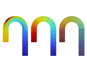
Figure 4. Spatial distribution of the transformation tensor $\overline{\overline {\boldsymbol{T^{\prime}}}}$ and its metamaterial microarray structures for steering the flow when the fluid-conveying pipeline is bent by 180°. (a–d) Spatial components of the transformation tensor $\overline{\overline {\boldsymbol{T^{\prime}}}}$. (e) Metamaterial element with an asymmetric array of elements tilted at an angle $\beta $ with respect to the principal axis of the microcell, which is determined by the bending angle of the pipeline.

3. Results and discussion

3.1. Circular-cross-section pipelines with arbitrary curvature

First, our study starts with a circular-cross-section pipeline with an arbitrary curvature to verify the validity of the proposed redirection theory. The characteristic length of all pipelines with circular cross-sections is L = 0.005 m. As shown in figure 5, the inlet is located at the left boundary of the pipeline, and the outlet is at the bottom. Furthermore, the remaining boundaries are set to be non-slip wall boundaries. In all working conditions, the difference between the inlet and outlet pressures of the pipeline is always 10 Pa. Therefore, the Reynolds number of the pressure-driven flow ranges from 750 to 1080. Figure 6 shows the computational configuration schemes for curved pipelines before and after application of the internal ‘hydrodynamic metamaterial steering theory’. It is well known that curved pipelines exhibit an unstable internal flow. However, the bending degree of the pipeline elbow significantly influences the flow state of the internal fluid. Hence, this study covers cases where the curvature angle varies from 60° to 180°. Figure 6(a) shows a curved pipeline before application of the steering theory proposed in this study. By contrast, figure 6(b) shows the scenario after this theory has been applied.

Figure 5. Schematics of pipelines with circular and square cross-sections, and corresponding computational meshes. (a) Schematic of a circular-cross-section curved pipeline, where L is the pipeline diameter and the bending angle varies. (b) Computational model of the circular-cross-section curved pipeline. (c) Surface mesh on the external wall surface. (d) Volume mesh inside the circular-cross-section pipeline. (e) Schematic of a square-cross-section curved pipeline, where L is the characteristic length of the pipeline and the bending angle varies. ( f) Computational model of the square-cross-section curved pipeline. (g) Surface mesh on the external wall surface. (h) Volume mesh inside the square-cross-section pipeline.

Figure 6. Computational configurations of curved pipelines with different bending degrees (60°–180°) (a) before and (b) after application of the hydrodynamic metamaterial steering theory.

In the study of pipeline flow, the viscous shear stress on the inner and outer walls of curved pipelines has always been the focus of attention, and it is also the leading cause of pipeline fatigue damage. Therefore, the shear stress on the walls of pipelines with different curvatures is first analysed. From the shear stress distribution on the outer wall of the curved pipeline (figure 7a), the shear stress is maximum in the elbow of the pipeline. With the increase in the elbow angle, the area over which the shear stress is maximum gradually increases, and the location of this area moves forward down the elbow. Since the difference between the inlet and outlet pressures is constant, the elbow length increases with increasing bending angle. Therefore, the buffer region of the internal flow of the pipeline at the elbow becomes longer, the viscous shear stress becomes more dispersed on the wall surface, and the peak value of the shear stress decreases.

Figure 7. Viscous shear stress distribution on the outer wall of pipelines with a bending angle ranging from 60° to 180°. ‘Dis’ represents the distance from the outlet along the outer profile; ‘L’ represents the characteristic diameter of the pipeline; ‘Outer_WSS’ represents the wall shear stress on the outer side of the bent pipeline surface.

To quantify the distribution of the shear stress on the outer wall of the pipeline, the shear stress values on the outermost profile of the pipeline are extracted and are shown in figure 7(b). The shear stress distribution on the outer wall reveals that in the inlet region, the wall shear stress is almost constant. As the fluid approaches the area, the shear stress gradually decreases due to the inertial centrifugal force of the fluid and the resistance generated by the bending of the pipeline. Inside the elbow region, the shear stress on the outer wall increases rapidly and reaches a peak value. As the flow leaves the elbow region, the outer wall shear stress gradually decreases again. However, the main difference is that with increasing bending angle, the maximum value of the shear stress gradually decreases and the peak in the distribution evolves into two separate peaks.

Next, the viscous shear stress on the inner wall of the pipeline is analysed. Compared with the shear stress distribution on the outer wall of the pipeline, the shear stress distribution on the inner wall is more complicated, as shown in figure 8(a,b). The shear stress on the inner wall reaches the maximum value as soon as the flow enters the elbow region, which corresponds to the trough in the shear stress distribution on the outer wall. Then, the shear stress on the inner wall reaches the first trough and the peak of the distribution on the outer wall occurs in the same section perpendicular to the centreline of the pipeline. Upon moving forward along the inner wall, due to the internal fluid backflow, the shear stress on the inner wall increases again and then gradually decreases until the flows exit the elbow region. When the flow approaches the end of the elbow region, the shear stress on the inner wall decreases rapidly and reaches the minimum, while the corresponding shear stress on the outer wall is maximum. Figure 8(b) also shows that when the bending angle is 60°, due to both the reduction in the total pipeline length and the small bending degree, the shear stress reaches the minimum at a later location along the inner wall and there are two almost identical minimum values.

Figure 8. Viscous shear force distribution on the inner wall of pipelines with bending angles ranging from 60° to 180°. ‘Dis’ represents the distance from the outlet along the inner profile; ‘Inner_WSS’ represents the wall shear stress on the inner side of the bent pipeline surface.

Figure 9(a) shows the cross-sectional pressure contours at $z = 0$ for pipelines with different bending angles. The pressure is concentrated on the outer wall of the elbow of the pipelines, as shown in figure 9(a). Moreover, the region in which the pressure is concentrated moves toward the entrance of the elbow region with the increase in the bending angle. The pressure distribution on the pipeline wall is shown in figure 27 the in Appendix. On the centreline of the pipeline, as shown in figure 9(b), the change in pressure field becomes less pronounced with increasing bending angle, but there is still a large unstable change in pressure in the elbow region.

Figure 9. Pressure distribution along the centreline of the curved pipelines with different bending angles.

Figure 10(a) depicts the velocity distribution in pipelines with different bending angles. The velocity distribution obeys the Poiseuille flow in the straight part of all pipelines. Upon approaching the elbow entrance, the curvature of the pipeline changes significantly. Due to the resistance exerted by the solid wall of the elbow, a high-speed zone is formed near the outer wall. Simultaneously, the flow is subjected to a centrifugal force at the elbow and is diverted towards the inner wall, leading to secondary backflow and flow separation. Figure 10(a) also shows that the backflow intensity is more prominent at a small bending angle. As the bending angle increases, the reflow intensity decreases gradually. This phenomenon occurs because the difference between the inlet and outlet pressures is assumed to be the same under all working conditions. The velocity curves in figure 10(b) show the same trend from a qualitative perspective.

Figure 10. Velocity distributions along the centreline of the curved pipelines with different bending angles.

Although the elbow-induced flow field has complex distribution features, its main characteristic is the radial pressure gradient generated by the centrifugal force on the fluid. Subjected to this inertial centrifugal force, the fluid along the centreline of the pipeline moves towards the outer wall. However, under the continuous action of the wall resistance, the fluid flows back from the outer wall to the inner wall; the flow field is thus severely distorted and a backflow field is generated, as shown schematically in figure 11(a,b).

Figure 11. Velocity isolines of the pipelines with different bending angles. (a) Velocity isolines on the cross-section at the centre of the elbow regions. (b) Velocity isolines at the exit of the elbow regions. The white dashed lines show the estimated secondary flow pattern. The black lines show the velocity contours and the numbers in the figure represent the velocity values.

These results show that the issues caused by pipeline elbows cannot be ignored. Figure 12(a–d) shows the flow field distribution in pipelines to which the hydrodynamic metamaterial theory has been applied. It can be seen from the pressure field shown in figure 12(a) that the radial pressure gradient created by the centrifugal force and wall resistance on the fluid in curved pipelines is eliminated effectively, which demonstrates the ability of the hydrodynamic metamaterial structures to steer and redirect the internal flow in curved pipelines. Increasing the bending angle of the curved pipelines does not affect their ability to redirect the flow. Compared with the pressure distribution in pipelines without hydrodynamic metamaterial structures, the problem of the pressure being concentrated in the wall of the elbow region of the curved pipelines is eliminated; this in turn effectively eliminates the resistance effect, thereby prolonging the service life of the pipeline. Moreover, the distribution of the pressure field across the entire curved pipelines becomes uniform.

Figure 12. Pressure and velocity fields of the pipelines after application of the hydrodynamic metamaterial steering theory proposed in this study. (a) Pressure and (b) velocity contours of the pipelines with different bending angles on the $z = 0$ cross-section. (c) Pressure and (d) velocity distributions along the centreline (black lines in panels (a) and (b), respectively) of the pipelines with different bending angles.

Figure 12(b) shows that the velocity field in the curved pipelines also turns into a steady flow state, with velocity contour lines being always parallel to the centreline instead of being severely distorted. At the same time, the backflow field is also completely eliminated regardless of the bending angle of the pipelines. These results demonstrate that the hydrodynamic metamaterial redirector can eliminate the energy and momentum loss of the fluid in curved pipelines. Thus, the safety of bent pipelines during use is improved.

Figure 12(c,d) shows the pressure and velocity distributions along the centreline of the curved pipelines. From the pressure distribution in figure 12(c), in the curved pipelines with the transformed hydrodynamic metamaterial structures, the pressure along the central axis of the pipeline decreases almost with a constant gradient from the inlet to the outlet. Notably, this pressure gradient gradually decreases as the bending angle increases. The velocity distribution in the entire curved pipelines is uniform, and the velocity along any line parallel to the pipeline axis is constant. Therefore, figure 12(d) proves that the secondary backflow phenomenon is eliminated. The details of the flow field results for curved pipelines before and after application of the transformed hydrodynamic metamaterial structures are shown in table 1, which demonstrate the effectiveness of the proposed strategy once again.

Table 1. Flow field results for curved pipelines (with different bending angles) to which the transformed hydrodynamic metamaterial structure has (values in the parentheses) and has not (values outside the parentheses) been applied.

*Notes: The velocity is taken along the centreline; ‘V’, ‘C’, ‘N’ and ‘Y’ stand for ‘varied’, ‘constant’, ‘No’ and ‘Yes’, respectively.

3.2. Square-cross-section pipelines with arbitrary curvature

Next, we investigate the effectiveness of the transformed hydrodynamic metamaterial structures for piping systems with a square cross-section, which are widely used in machinery and integrated circuits. The characteristic length L of all pipelines with square cross-sections is 0.005 m. For the flow in these pipelines, we still set the difference between the inlet and outlet pressures of the pipelines to be 10 Pa, which is the same as that of the pipelines with circular cross-sections. The Reynolds number of this pressure-driven flow ranges from 850 to 1150. The viscous shear stress distribution on the wall of the square-cross-section pipelines reveals that the shear stress is concentrated at the elbow also in this case. Compared with circular-cross-section pipelines, square-cross-section pipelines are subjected to the influence of the corners, as shown in figure 13(a). The corners have a significant impact on the internal flow. Due to the presence of the corners, the distribution of the shear stress on the outer wall of these pipelines is no longer as smooth as that of the circular-cross-section pipelines, and the peak values of the shear stress for different bending angles are larger than in the previous case. However, especially in the elbow regions, the shear stress in the corners is minimal, causing a sizeable shear moment between the outer wall and the corner of the pipeline. The shear effect on the pipeline wall is an important factor in determining the pipeline fatigue damage.

Figure 13. Viscous shear force distributions along the outer and inner bent walls of the square-cross-section pipelines with different bending angles.

As shown in figure 13(b,c), the variation in the wall viscous shear stress along the centrelines of the outer and inner walls of the square-cross-section pipelines is the same as that of the circular-cross-section pipelines, except that the peak and trough values of the former are larger than those of the latter. Table 2 presents a comparison of the flow field results for the two types of pipelines. From table 2, it can be inferred that the presence of corners in the square-cross-section pipelines is likely to lead to stress concentration and secondary backflow phenomena at the elbow.

Table 2. Comparison of the flow field results for the circular-cross-section (values outside the parentheses) and square-cross-section (values in the parentheses) pipelines with different bending angles.

Figure 14 shows that the distribution of the pressure field in the curved, square-cross-section pipelines before and after application of the hydrodynamic metamaterial steering theory. When the transformed hydrodynamic structures are not applied, pressure stress concentration occurs at the elbow. The pressure isolines shown in figure 14(a) are curved. Since circular-cross-section pipelines change their shape smoothly, the pressure field distribution is relatively uniform. However, this is not the case for square-cross-section pipelines: the pressure field on their wall is no longer uniform, especially at the corners, as shown in figure 28 in the Appendix. It can be seen from figure 14(b) that the radial pressure gradient created by the centrifugal force and wall resistance on the fluid in the curved, square-cross-section pipelines is also eliminated effectively, which once more demonstrates the ability of the hydrodynamic metamaterial structures to steer and redirect the internal flow in curved pipelines. Increasing the bending angle does not affect the ability of the hydrodynamic metamaterial structures to redirect the flow also in this case.

Figure 14. Distribution of the pressure field in the square-cross-section pipelines with different bending angles (a) before and (b) after application of the hydrodynamic metamaterial steering theory.

Figure 15 shows the pressure field distribution along the central axis of the curved, square-cross-section pipelines without and with the hydrodynamic metamaterial structures. The pressure field is not uniformly distributed in the pipelines when the metamaterial structures have not been applied, especially in the elbow region. When the metamaterial structures are arranged inside the pipelines, the pressure field decreases with a constant gradient along the central axis of the pipeline between the inlet and outlet. From the pressure field distribution of the square-cross-section pipelines, it can be concluded that the hydrodynamic metamaterial steering theory is valid regardless of the bending angle and cross-sectional shape of the pipeline. Moreover, we can see that the pressure gradient decreases with the increase in the bending angle, which is still caused by the constant difference between the inlet and outlet pressures under all working conditions.

Figure 15. Comparison of the pressure along the centrelines of square-cross-section pipelines with different bending angles before and after application of the hydrodynamic metamaterial steering theory.

The velocity field distributions of the curved, square-cross-section pipelines before and after application of the hydrodynamic transformation theory are shown in figure 16. Figure 16(a) shows the flow streamlines of the curved, square-cross-section pipelines with different bending angles without the metamaterial structures. The flow spirals in these pipelines. With the increase in the pipeline bending angle and length, the intensity of this velocity turbulence gradually decreases. By contrast, the flow streamlines of the curved, square-cross-section pipelines to which the redirection theory has been applied are evenly distributed, as shown in figure 16(b). These streamlines are always parallel to the pipeline central axis, proving the generality of the flow steering theory proposed in this study once more.

Figure 16. Flow streamlines in curved, square-cross-section pipelines with different bending angles (a) before and (b) after application of the hydrodynamic metamaterial steering theory.

The elbow-induced flow field has a more complex distribution in the curved, square-cross-section pipelines than in the circular-cross-section pipelines due to the presence of the corners. The radial pressure gradient generated by the centrifugal force on the fluid is greater than that of the circular-cross-section pipelines. Driven by the inertial centrifugal force and wall resistance, the main flow along the central axis moves first outward and then inward. Furthermore, the flow field is severely distorted, giving rise to a backflow field, which is marked by the white dashed lines in figure 17(a,b).

Figure 17. Velocity contours of the curved, square-cross-section pipelines with different bending angles. (a) Velocity contours on the central cross section of the elbows. (b) Velocity contours on the cross-section at the exit of the elbows. (c) Velocity contours on the central cross-section of the elbows after applying the hydrodynamic metamaterial theory. The white dashed lines show the estimated secondary flow pattern. The black lines show the velocity contours and the numbers in the figure represent the velocity values.

Figure 17(c) shows the velocity distribution on the central cross-section of the elbow of the curved, square-cross-section pipelines with different bending angles once the hydrodynamic metamaterial theory has been applied. The velocity contours in the figure take the shape of regular rings around the centre and then become more squared, resembling the pipeline shape, with the velocity values varying with the bending angle. These results demonstrate that the hydrodynamic metamaterial structures effectively eliminate the secondary backflow phenomenon caused by pipeline elbows. Moreover, the influence of the corners is also reduced.

To analyse the distribution of the velocity field in the curved, square-cross-section pipelines with and without the hydrodynamic metamaterial structures from an overall perspective, we here consider once more the velocity distribution on the central axis, as shown in figure 18. For the velocity field distribution without the metamaterial structures, the velocity changes when the flow approaches the elbow region, and such a change affects the whole elbow and its downstream region. It can also be seen that as the bending angle increases, the high-speed zone in the bend region moves forward and the velocity amplitude decreases.

Figure 18. Comparison of the velocity along the centreline of square-cross-section pipelines with different bending angles before and after application of the hydrodynamic metamaterial steering theory.

By contrast, in the curved square-cross-section pipelines to which the metamaterial theory has been applied, the velocity field remains basically constant. In particular, the velocity field upstream and downstream of the elbow is uniform and takes equal values. In the elbow region, after placing the metamaterial structures inside the pipeline, the internal flow field also becomes uniform, as shown by the dotted lines in figure 18. In addition, we can also observe that the metamaterial steering structures work in the same way regardless of the elbow angle.

3.3. Right-angle pipelines

In practical applications, due to the spatial constraints imposed by the mechanical equipment and the structure of the cooling systems, it is often necessary to use right-angle pipelines. This adds complexity to the flow in circular-cross-section, right-angle pipelines compared with the case where there is a gradual bent (i.e. the elbow). However, the flow in rectangular-cross-section, right-angle pipelines is even more complicated than that in circular-cross-section, right-angle pipelines due to the presence of the corners. Thus, we selected this more complex structure for study.

In this computational case, the characteristic length L of the pipelines is 0.01 m and the height is d = L/2, as shown in figure 19(a). Since the right-angle-elbow area is the region where the hydrodynamic metamaterial structures are applied, i.e. the region where the transformed density and dynamic viscosity are obtained, the mesh in this area is refined, as shown in figure 19(b). Figure 19(c) shows the distribution of the viscous shear stress on the pipeline wall, which illustrates that the stress is concentrated at the right-angle corner.

Figure 19. Computational configuration and corresponding results for rectangular-cross-section, right-angle pipelines. (a) Schematic of the geometry of a square-cross-section, right-angle pipeline and (b) corresponding computational mesh. (c) Shear stress distribution on the pipeline wall.

Figure 20(a,b) shows the pressure profiles in the square-cross-section, right-angle pipeline without and with the hydrodynamic metamaterial steering structures, respectively. When the hydrodynamic metamaterial steering structures are not present, the pressure field distribution on the pipeline surface is not uniform. The pipeline wall perpendicular to the main flow direction shown in figure 20(a) exhibits a local stress concentration area. The pressure isosurfaces inside the pipeline present a spatial curl, which is consistent with the black curve in figure 21(a). By contrast, the pressure distribution on the pipeline wall becomes uniform when adopting the hydrodynamic metamaterial steering structures. The pressure isosurfaces inside the pipeline become planar. In addition, the pressure along the central axis decreases with a constant gradient, as shown by the red curve in figure 21(a).

Figure 20. Profiles of the pressure and velocity fields in the square-cross-section, right-angle pipeline without and with the hydrodynamic metamaterial steering structures. Distribution of the pressure field on the pipeline surface and pressure contour in the pipeline (a) before and (b) after application of the hydrodynamic metamaterial steering theory. Distribution of the velocity field on the pipeline surface and pressure contour in the pipeline (c) before and (d) after application of the hydrodynamic metamaterial steering theory. The black lines show the velocity contours, and the numbers in the figure represent the velocity values.

Figure 21. Comparison of the pressure and velocity along the central axis of the right-angle pipeline before and after application of the hydrodynamic metamaterial steering theory. Here, ‘d’ is the height of the right-angle pipeline shown in figure 19(a).

Regarding the velocity field inside the pipeline, due to the increase in the cross-section area of the pipeline joint, a low-velocity zone is formed at the upper right corner of the pipeline, as shown by the top right subfigure of figure 20(c). Then, due to the sudden change in the shape of the pipeline and the wall resistance perpendicular to the main flow direction, the flow first moves towards the outer wall and then toward the inner wall, as shown by the bottom right subfigure of figure 20(c). To study the flow field in the pipeline from a more quantitative point of view, the velocity distribution on the centreline of the pipeline is analysed. The black curve in figure 21(b) shows that the velocity field is first uniformly distributed in the entrance region of the right-angle pipeline. When approaching the right-angle joint, the velocity first decreases and then increases due to the sudden expansion of the pipeline cross-section. The velocity sharply decreases when the flow exits the right-angle joint due to the wall resistance being perpendicular to the main flow direction. With increasing distance from the right-angle joint, the influence of the right-angle joint decreases, and the velocity increases gradually.

Figure 20(d) shows that after applying the hydrodynamic metamaterial theory, the turbulent velocity field inside the pipeline becomes uniform. Furthermore, the velocity isolines become uniform rings. However, due to the sudden expansion of the cross-section area at the joint, there will still be a low-speed zone, which corresponds to the trough of the red curve shown in figure 21(b). In addition, we can see two segments in which the velocity is perturbed on the red curve in figure 21(b), where the fluid flows in and out of the right-angle joint. It is the right angle of the joint and the corners of the pipeline that cause this phenomenon. However, we can still see that the flow field is well controlled with the added metamaterial structures.

4. Hydrodynamic metamaterial implementation

From the expression of the transformation tensor, we can see that the elements of the transformation tensor matrix $\overline{\overline {\boldsymbol{T^{\prime}}}}$ change continuously depending on the distance r from the centre of curvature of the curved pipelines, as shown in (4.1). Due to the existence of non-diagonal elements in the transformation matrix $\overline{\overline {\boldsymbol{T^{\prime}}}}$, the design and manufacturing process of metamaterials is extremely complex. Through careful observation, we can find that the transformation tensor is a real symmetric matrix, which can be diagonalized using the matrix theory, thereby reducing the complexity of the metamaterial design.

(4.1) \begin{equation} \overline{\overline {\boldsymbol{T^{\prime}}}} = \left[ {\begin{array}{@{\,}ccc@{}} {\overline{\overline {T^{\prime}_{xx}}} } & {\overline{\overline {{T^{\prime}_{xy}}}} } & 0\\ {\overline{\overline {{T^{\prime}_{yx}}}} } & {\overline{\overline {T^{\prime}_{yy}}} } & 0\\ 0 & 0 & {\overline{\overline {T^{\prime}_{zz}}} } \end{array}} \right] = \;\left[ {\begin{array}{@{}ccc@{}} {\dfrac{{{l^2}{{y^{\prime}}^2} + {{x^{\prime}}^2}{r^2}{\alpha^2}}}{{l{r^3}\alpha }}} & { - \dfrac{{x^{\prime}y^{\prime}({l^2} - {r^2}{\alpha^2})}}{{l{r^3}\alpha }}} & 0\\ { - \dfrac{{x^{\prime}y^{\prime}({l^2} - {r^2}{\alpha^2})}}{{l{r^3}\alpha }}} & {\dfrac{{{l^2}{{x^{\prime}}^2} + {{y^{\prime}}^2}{r^2}{\alpha^2}}}{{l{r^3}\alpha }}} & 0\\ 0 & 0 & {\dfrac{{\alpha r}}{l}} \end{array}} \right].\end{equation}

We now return to (4.1) to demonstrate how it can be used to implement the fluid flow steering metamaterial. According to the matrix theory, (4.1) can be diagonalized as

(4.2)\begin{gather}\left[ {\begin{array}{@{\,}ccc@{}} {\overline{\overline {{T^{\prime}_u}}} } & 0 & 0\\ 0 & {\overline{\overline {{T^{\prime}_v}}} } & 0\\ 0 & 0 & {\overline{\overline {{T^{\prime}_w}}} } \end{array}} \right],\end{gather}

(4.3)\begin{gather}\overline{\overline {{T^{\prime}_u}}} = \frac{1}{2}\left( {\overline{\overline {T^{\prime}_{xx}}} + \overline{\overline {T^{\prime}_{yy}}} - \sqrt {{{\overline{\overline {T^{\prime}_{xx}}} }^2} + 4\overline{\overline {{T^{\prime}_{xy}}}} \overline{\overline {{T^{\prime}_{yx}}}} - 2\overline{\overline {T^{\prime}_{xx}}} \overline{\overline {T^{\prime}_{yy}}} + {{\overline{\overline {T^{\prime}_{yy}}} }^2}} } \right),\end{gather}

(4.4)\begin{gather}\overline{\overline {{T^{\prime}_v}}} = \frac{1}{2}\left( {\overline{\overline {T^{\prime}_{xx}}} + \overline{\overline {T^{\prime}_{yy}}} + \sqrt {{{\overline{\overline {T^{\prime}_{xx}}} }^2} + 4\overline{\overline {{T^{\prime}_{xy}}}} \overline{\overline {{T^{\prime}_{yx}}}} - 2\overline{\overline {T^{\prime}_{xx}}} \overline{\overline {T^{\prime}_{yy}}} + {{\overline{\overline {T^{\prime}_{yy}}} }^2}} } \right),\end{gather}

(4.5)\begin{gather}\overline{\overline {{T^{\prime}_w}}} = \overline{\overline {T^{\prime}_{zz}}} \textrm{ }.\end{gather}

According to the equivalence relationship between the diagonalized transformation matrix and the original transformation matrix, we can obtain

(4.6) \begin{align}\left[ {\begin{array}{@{\,}ccc@{}} {\overline{\overline {T^{\prime}_{xx}}} } & {\overline{\overline {{T^{\prime}_{xy}}}} } & 0\\ {\overline{\overline {{T^{\prime}_{yx}}}} } & {\overline{\overline {T^{\prime}_{yy}}} } & 0\\ 0 & 0 & {\overline{\overline {T^{\prime}_{zz}}} } \end{array}} \right] = \left[ {\begin{array}{@{}ccc@{}} {\textrm{cos}\left( {\dfrac{\tau }{2}} \right)} & { - \textrm{sin}\left( {\dfrac{\tau }{2}} \right)} & 0\\ {\textrm{sin}\left( {\dfrac{\tau }{2}} \right)} & {\textrm{cos}\left( {\dfrac{\tau }{2}} \right)} & 0\\ 0 & 0 & 1 \end{array}} \right]\left[ {\begin{array}{@{\,}ccc@{}} {\overline{\overline {{T^{\prime}_u}}} } & 0 & 0\\ 0 & {\overline{\overline {{T^{\prime}_v}}} } & 0\\ 0 & 0 & {\overline{\overline {{T^{\prime}_w}}} } \end{array}} \right]\left[ {\begin{array}{@{}ccc@{}} {\textrm{cos}\left( {\dfrac{\tau }{2}} \right)} & {\textrm{sin}\left( {\dfrac{\tau }{2}} \right)} & 0\\ { - \textrm{sin}\left( {\dfrac{\tau }{2}} \right)} & {\textrm{cos}\left( {\dfrac{\tau }{2}} \right)} & 0\\ 0 & 0 & 1 \end{array}} \right]\textrm{ }.\end{align}

From (4.6), we get

(4.7)\begin{align} & \overline{\overline {{T^{\prime}_u}}} \,\textrm{co}{\textrm{s}^2}\left( {\dfrac{\tau }{2}} \right) + \overline{\overline {{T^{\prime}_v}}} \,\textrm{si}{\textrm{n}^2}\left( {\dfrac{\tau }{2}} \right) = \overline{\overline {{T^{\prime}_u}}} \dfrac{{1 + \textrm{cos}(\tau )}}{2} + \overline{\overline {{T^{\prime}_v}}} \dfrac{{1 - \textrm{cos}(\tau )}}{2}\nonumber\\ & \quad = \dfrac{{\overline{\overline {{T^{\prime}_u}}} + \overline{\overline {{T^{\prime}_v}}} }}{2} + \dfrac{{\overline{\overline {{T^{\prime}_u}}} - \overline{\overline {{T^{\prime}_v}}} }}{2}\,\textrm{cos}(\tau ) = \dfrac{{{l^2}{{y^{\prime}}^2} + {{x^{\prime}}^2}{r^2}{\alpha ^2}}}{{l{r^3}\alpha }}, \end{align}

(4.8)\begin{align} & \overline{\overline {{T^{\prime}_u}}} \,\textrm{cos}\left( {\dfrac{\tau }{2}} \right)\,\textrm{sin}\left( {\dfrac{\tau }{2}} \right) - \overline{\overline {{T^{\prime}_v}}} \,\textrm{cos}\left( {\dfrac{\tau }{2}} \right)\,\textrm{sin}\left( {\dfrac{\tau }{2}} \right) = ({\overline{\overline {{T^{\prime}_u}}} - \overline{\overline {{T^{\prime}_v}}} } )\textrm{cos}\left( {\dfrac{\tau }{2}} \right)\textrm{sin}\left( {\dfrac{\tau }{2}} \right)\nonumber\\ & \quad = \dfrac{{\overline{\overline {{T^{\prime}_u}}} - \overline{\overline {{T^{\prime}_v}}} }}{2}\,\textrm{sin}(\tau ) ={-} \dfrac{{x^{\prime}y^{\prime}({l^2} - {r^2}{\alpha ^2})}}{{l{r^3}\alpha }}, \end{align}

(4.9)\begin{align} & \overline{\overline {{T^{\prime}_u}}} \,\textrm{si}{\textrm{n}^2}\left( {\dfrac{\tau }{2}} \right) + \overline{\overline {{T^{\prime}_v}}} \,\textrm{co}{\textrm{s}^2}\left( {\dfrac{\tau }{2}} \right) = \overline{\overline {{T^{\prime}_u}}} \dfrac{{1 - \textrm{cos}(\tau )}}{2} + \overline{\overline {{T^{\prime}_v}}} \dfrac{{1 + \textrm{cos}(\tau )}}{2}\nonumber\\ & \quad = \dfrac{{\overline{\overline {{T^{\prime}_u}}} + \overline{\overline {{T^{\prime}_v}}} }}{2} + \dfrac{{\overline{\overline {{T^{\prime}_v}}} - \overline{\overline {{T^{\prime}_u}}} }}{2}\,\textrm{cos}(\tau ) = \dfrac{{{l^2}{{x^{\prime}}^2} + {{y^{\prime}}^2}{r^2}{\alpha ^2}}}{{l{r^3}\alpha }}. \end{align}

By combining (4.7), (4.8) and (4.9), we can obtain

(4.10) \begin{equation}\left. {\begin{array}{c@{}} {\overline{\overline {{T^{\prime}_u}}} = \overline{\overline {{T^{\prime}_w}}} = \overline{\overline {T^{\prime}_{zz}}} = \dfrac{{\alpha r}}{l},}\\ {\overline{\overline {{T^{\prime}_v}}} = \dfrac{l}{{\alpha r}},}\\ {\textrm{cos}(\tau ) = \textrm{cos}(2\theta ),\quad \textrm{sin}(\tau ) = \textrm{sin}(2\theta ).} \end{array}} \right\}\end{equation}

Therefore, $\overline{\overline {{T^{\prime}_u}}}$, $\overline{\overline {{T^{\prime}_v}}}$ and $\overline{\overline {{T^{\prime}_w}}}$ are the principal values along the coordinate system transformed according to the matrix theory. Here, a micropillar array tilted by an angle $\beta = (\tau /2) = \theta$ is formed, where $\theta $ is the angle between the new principal axes and the original coordinate axes. In addition, for a pipeline with a specific curvature angle, $\alpha$ and l are both constant values. Therefore, the transformation tensor components $\overline{\overline {{T^{\prime}_u}}}$, $\overline{\overline {{T^{\prime}_v}}}$ and $\overline{\overline {{T^{\prime}_w}}}$ are only related to the distance r from the curvature centre.

Up to now, the transformation matrix tensor $\overline{\overline {T^{\prime}}}$ has been simplified from a tensor containing five non-diagonal elements to a transformation matrix with only three diagonal elements, which reduces significantly the complexity of the design and fabrication of hydrodynamic steering metamaterials. However, as shown in figure 22(a−c), the transformation tensor components $\overline{\overline {{T^{\prime}_u}}}$, $\overline{\overline {{T^{\prime}_v}}}$ and $\overline{\overline {{T^{\prime}_w}}}$ still exhibit spatial anisotropy, and the actual realization of hydrodynamic metamaterials remains challenging. Equation (4.10) and figure 22(a,c) indicate that $\overline{\overline {{T^{\prime}_u}}}$ and $\overline{\overline {{T^{\prime}_w}}}$ have the same properties, permitting us to focus on only one of them. The red curves in figure 22(d,e) show that the $\overline{\overline {{T^{\prime}_u}}}$ and $\overline{\overline {{T^{\prime}_v}}}$ values vary with increasing distance r outward from the curvature centre of the curved pipeline. The only difference is that while $\overline{\overline {{T^{\prime}_u}}}$ increases linearly with the increase in r, $\overline{\overline {{T^{\prime}_v}}}$ decreases with the increase in r; the variation gradient decreases gradually. From a more quantitative perspective, $\overline{\overline {{T^{\prime}_u}}}$ and $\overline{\overline {{T^{\prime}_v}}}$ are reciprocals of each other.

Figure 22. Spatial distribution of the diagonalized transformation tensor $\overline{\overline {T^{\prime}}}$. (a−c) Spatial components $\overline{\overline {{T^{\prime}_u}}}$, $\overline{\overline {{T^{\prime}_v}}}$ and $\overline{\overline {{T^{\prime}_w}}}$ along the diagonalized principal axes u, v and w, respectively. (d,e) Multilayer piecewise homogenization components along their corresponding diagonalized principal axes.

As a preliminary step to designing the hydrodynamic metamaterial steering structure, it is necessary to compartmentalize the steering structure to approximate the values of the transformation tensor components required for implementation, as shown in figure 22(d,e). The number of multilayers of the hydrodynamic metamaterial steering structure can be adjusted as desired. However, we know that a greater number of segments means the closer the steering effect is to the original anisotropic transformation tensor. Using a piecewise integral approximation method, this metamaterial can be designed hierarchically by employing the average values of the components of the piecewise integral approximation transformation tensor. In each layer, isotropic materials with spatially uniform properties can be achieved, as shown in table 3. Figure 23 shows the pressure and velocity fields of the multilayer hydrodynamic metamaterial steering structure, which still generates the desired physical field while considerably simplifying the fabrication process.

Table 3. Multilayer components $\overline{\overline {{T^{\prime}_u}}}$, $\overline{\overline {{T^{\prime}_v}}}$ and $\overline{\overline {{T^{\prime}_w}}}$ on each compartmentalized layer.

Figure 23. Distribution of the pressure and velocity fields under different conditions. (a) Simulation results of the pressure and velocity fields using the diagonalized tensor components $\overline{\overline {{T^{\prime}_u}}}$, $\overline{\overline {{T^{\prime}_v}}}$ and $\overline{\overline {{T^{\prime}_w}}}$. (b) Simulation results of the pressure and velocity fields using the multilayer diagonalized tensor components. (c) Pressure and (d) velocity fields for the diagonalized tensor components and the multilayer diagonalized tensor components, respectively.

As shown in figure 24, the hydrodynamic metamaterial steering structure is divided into multiple evenly spaced concentric half-rings. Isotropic micropillar array structures with spatially uniform properties can be achieved in each layer. Characterizing the hydrodynamic performance of the micropillar is the key to designing the hydrodynamic metamaterial steering structure. Studies on porous media fluid mechanics have shown that an effective hydrodynamic performance can be achieved (Breugem 2007; Yazdchi et al. 2011; Hale et al. 2014). This method is one of the most commonly used and powerful approaches to characterize the hydrodynamic performance of microelement array structures; it involves computing the macroscopic hydrodynamic performance of the micropillar array while taking into account their microstructure. For the hydrodynamic metamaterial micropillar array to be studied, the cross-sectional shapes (rectangular pillar, elliptical pillar and cylindrical pillar) of the metamaterial microstructures and the characteristic dimensions (${l_x}$, ${l_y}$ and ${l_z}$, or a and $b$) of the micropillars determine the effective hydrodynamic performance of the cell structure, which is shown in step 1 in figure 24. Therefore, it is crucial to understand the quantitative relationship between the geometric characteristics of micropillars (micropillar shapes and geometric characteristic dimensions) and their effective hydrodynamic performance.

(4.11)\begin{gather}{\boldsymbol{T}_{effective,i}} = \left( {\frac{{\langle {\boldsymbol{V}_0}\rangle }}{{\langle {\boldsymbol{V}_{pillar }}\rangle }}} \right){\boldsymbol{T}_i},\quad i = u,v,w.\end{gather}

(4.12)\begin{gather}{\boldsymbol{V}_0} = \frac{1}{V}\int_{{V_f}} {\boldsymbol{u}\,\textrm{d}v} ,\end{gather}

where ${\boldsymbol{T}_{effective,i}}$, ${\boldsymbol{T}_{\boldsymbol{i}}}$, $\boldsymbol{u}$, $\langle {\boldsymbol{V}_0}\rangle$, $\textrm{V}$ and ${V_f}$ are the effective hydrodynamic coefficients, original hydrodynamic coefficients (i.e. fluidic density and dynamic viscosity), local microscopic velocity of the fluid, corresponding averaged velocity, total volume and volume of the fluid, respectively.

Figure 24. Schematic illustrating the steps required for establishing a multilayer hydrodynamic metamaterial steering structure model for a curved square pipeline with a 180° bending angle.

In addition, however, it is indispensable to incorporate the tilt angle $\beta = (\tau /2)$, which represents the angle between the original coordinate principal axes and the rotation-transformed principal axes. Step 2 in figure 24 depicts the corresponding relationship for the principal axes before and after diagonalization. For the theoretical design, a micropillar array with an evenly spaced set of distances was chosen so that an integer number of unit cells fits exactly around the circumference of each half-ring. It is established that the rotation angle is positive counterclockwise and negative clockwise. Step 3 in figure 24 depicts the macroscopic hydrodynamic metamaterial steering structure and the microscopic micropillar array.

To establish the hydrodynamic metamaterial steering structure for numerical simulations, the transformed tensor components should be scaled up to be larger than 1.0 (the factor of the natural fluidic viscosity). This is because when we use metamaterial micro-unit structures to alter the flow field, the effective hydrodynamic viscosity generated is always greater than 1.0. Therefore, the diagonalized transformation tensor elements in table 3 can be scaled up by a factor of 2.1. For impedance matching with the natural fluid flowing in the pipelines, the background fluid field should also be scaled up by a factor of 2.1. In fact, this coefficient can be adjusted as desired, but it should not be less than 1.0. Equation (4.10) and figure 22(a,c) indicate that $\overline{\overline {{T^{\prime}_u}}}$ and $\overline{\overline {{T^{\prime}_w}}}$ have the same properties, permitting us to focus on $\overline{\overline {{T^{\prime}_u}}}$ and $\overline{\overline {{T^{\prime}_v}}}$, as shown in table 4.

Table 4. Multilayered components $\overline{\overline {{T^{\prime}_u}}}$ and $\overline{\overline {{T^{\prime}_v}}}$ scaled up on each compartmentalized layer.

In our study, the evenly spaced set of ‘fanlike’ shapes are approximated by square elements. In addition, the rectangular micropillar unit can be selected as the inserted microelement in the hydrodynamic metamaterial steering structure. The micropillar array shown in figure 25(a) is the hydrodynamic metamaterial steering microstructure we seek to manipulate the fluid flow as desired. There are several techniques that can be used to fabricate hydrodynamic metamaterials, such as soft lithography, 3-D printing and microfabrication. By using soft lithography technology or 3-D printing technology, the hydrodynamic metamaterial microstructure in a pipeline required to manipulate the fluid flow path in actual engineering can be achieved. Figure 25(a) shows the ten-layer micropillar array structure to construct the hydrodynamic metamaterial steering structure with multiple evenly spaced concentric half-rings. From the inside to the outside, the number of cells in each half-ring is 39, 42, 46, 49, 52, 55, 58, 61, 64 and 67. The entire background flow field is filled with 179 μm diameter cylinders inserted for impedance matching. The length of the micropillars (x_l and y_l) are present in table 5. Figure 25(b) shows a micropillar array (and corresponding magnified view) with an unstructured mesh on the middle section of a square-cross-section curved pipeline. A large number of free tetrahedral grids are required because the models contain very fine structures. The boundary layer grid consists of ten layers, where the stretching factor is 1.2, Y plus is 1.0 and the mesh growth rate is 1.2. The total number of meshes is approximately 18 million.

Figure 25. Constructed micropillar array model and corresponding computational meshes. (a) Design of the pillar-arrayed hydrodynamic metamaterial steering structure with the magnified view showing its detailed configuration. (b) Unstructured mesh on the middle section of a square-cross-section curved pipeline and corresponding magnified view.

Table 5. Multilayered components $\overline{\overline {{T^{\prime}_u}}}$ and $\overline{\overline {{T^{\prime}_v}}}$ scaled up by a factor of 2.1 and corresponding micropillar dimensions for each compartmentalized layer.

In this section, the characteristic dimension of the pipelines with square cross-sections is L = 0.005 m. A constant water viscosity (μ = 0.001 Pa s) and density (ρ = 1000 kg m⁻³) are set. We still set the pressure difference between the inlet and outlet of all pipelines to be 10 Pa. Non-slip boundary conditions were applied to all surfaces of the microstructures, including the cylinder and micropillars. When the hydrodynamic metamaterial micropillars are inserted into the pipeline, the Reynolds number of this pressure-driven flow is approximately $Re = \rho \boldsymbol{V}L/\mu = 100$. Figure 26(a,d) show the simulation results of the pressure field for the hydrodynamic metamaterial steering structure. As shown in figure 26(a), the pressure field in the bent pipeline varies smoothly, although the pipeline has a 180° bending angle. Figure 26(d) shows that the pressure contours in the bent pipeline remain straight. These findings validate the effectiveness of the hydrodynamic metamaterial steering structure.

Figure 26. Simulated pressure field for the hydrodynamic metamaterial steering structure. (a) Simulated pressure field for the pillar-arrayed hydrodynamic metamaterial steering structure and three magnified views of the bending elbow. Distribution of the pressure field in the square-cross-section pipelines (b) before and (c) after application of the hydrodynamic metamaterial steering theory. (d) Simulated pressure contours (the pink lines) for the pillar-arrayed hydrodynamic metamaterial steering structure.

Figure 26(b,c) shows the distribution of the pressure field in the square-cross-section pipelines before and after application of the hydrodynamic metamaterial steering theory, respectively. When the transformed hydrodynamic structures are not applied, pressure stress concentration occurs at the elbow. The pressure isolines shown in figure 26(b) are curved. From figure 26(c), the radial pressure gradient created by the centrifugal force and wall resistance on the fluid in the curved, square-cross-section pipelines is also eliminated effectively, which once more demonstrates the ability of the hydrodynamic metamaterial structures to steer and redirect the internal flow in curved pipelines.

5. Conclusion

In this study, an innovative strategy based on the Navier–Stokes equations was proposed for steering and redirecting the flow in pipelines with arbitrary curvature. This theoretical approach eliminates the problems of the secondary backflow and wall stress concentration caused by the presence of elbows with arbitrary curvature in the pipelines. The hydrodynamic metamaterial structures designed for curved, rectangular-cross-section pipelines eliminate the complex flow instability caused by the change in pipeline curvature as well as the influence of the pipeline corners. The hydrodynamic metamaterial structures required to eliminate these influences were provided through a detailed theoretical comparative study of the flow in curved pipelines (with bending angles in the range of 60°–180°) with circular and rectangular cross-sections.

Furthermore, metamaterial structures based on this theory for pipelines with abrupt shape changes and corner effects were designed. The effectiveness of the analytical design of metamaterial structures for right-angle pipelines was verified from both qualitative and quantitative perspectives. The proposed approach for steering and redirecting flow is asymptotically perfect and physically achievable. It is suitable for controlling the internal flow in pipelines with arbitrary shape and curvature.

As aforementioned, hydrodynamic metamaterial steering structures are artificial composites that possess properties that are different from those of conventional materials; such unusual properties originate from the geometry structures of the microstructural units rather than their individual components. The hydrodynamic metamaterial structure is only a micropillar structure placed in the interior of the pipeline, which does not change the physical properties of the fluid flowing around it. Using the soft lithography technology or the 3-D printing technology, the hydrodynamic metamaterial microstructure required to manipulate the fluid flow path in actual engineering applications can be achieved.