I. INTRODUCTION
With a large amount of service providers and retailers going online, web users are faced with a daunting task of sifting through a barrage of items and information to find the preferred product or service. The need to improve customer's experience, which in effect increases the popularity and hence profits of online portals have led to widespread interest in design of efficient recommender systems (RSs) in the recent times [Reference Resnick, Iacovou, Suchak, Bergstrom and Riedl1–Reference Miller, Albert, Lam, Konstan and Riedl3]. RSs utilize information collected in the past about users to make personalized recommendation, so that they are presented with select choices most relevant to their interest area.
The current de facto approach for the RS design is collaborative filtering (CF) [Reference Su and Khoshgoftaar4–Reference Lee, Sun and Lebanon6]. Most CF techniques primarily work with the explicit feedback (ratings say on a scale of 1–5) provided by customers on previously purchased items. Some works [Reference Hu, Koren and Volinsky7] rely on implicit information as well such as browsing history or buying patterns of users for rating prediction. Explicit ratings, though hard to acquire (as it requires user's active participation) are more reliable than the implicitly gathered information. Also, implied data are unable to capture negative feedback, e.g. if a person does not buy an item, it is difficult to decide if he/she dislikes the items or does not know of the item. In this work, we will use explicit ratings given by users as the primary data source.
CF models basically rest on the assumption that if two users rate a few items similarly, they will most probably rate others also in similar fashion. This belief can be exploited in two ways – memory (or neighborhood)-based approach and latent factor model-based approach.
Memory-based methods [Reference Desrosiers, Karypis, Ricci, Rokach, Shapira and Kantor8,Reference Jeong, Lee and Cho9] are heuristic interpolation strategies that make use of the entire rating matrix (available database) to find the neighbors of a user for whom prediction is to be made. Predicted rating of an item for the target user is governed by the ratings given to the item under consideration by its nearest-k neighbors (users). The approach can be extended to the item-centric design also, which focuses on finding similar items (instead of users) [Reference Gao, Wu and Jiang10]. However, these methods are slow, lack good accuracy, and are unable to provide adequate coverage [Reference Adomavicius and Tuzhilin11].
On the other hand (latent factor), model-based methods [Reference Hofmann12,Reference Yu, Lin, Wang, Wang and Wang13] perform better in terms of quality of prediction (QoP) and sparsity challenge [Reference Adomavicius and Tuzhilin11], but lacks the ease of interpretability embedded in the memory-based approach. Model-based techniques fundamentally represent the available information in the form of a lower-dimensional structure under the proposition that the overall rating matrix can be represented by a relatively small number of independent variables or latent factors [Reference Hofmann12]. It can be safely considered that an item can be defined by a certain limited number of variables or latent factor, like for a movie they could be genre, cast, and director. Furthermore, a user displays preference toward or against these traits. The likelihood of a user preferring a particular item is nothing but the interaction between their individual latent factor vectors. Under this assumption, users can be modeled as a vector describing his/her affinity to the latent factors and items by their degree of possession of the corresponding latent factors.
The most commonly used formulation for latent factor framework-based design is the matrix factorization (MF) [Reference Koren, Bell and Volinsky14]. Several works have focused on the design of efficient algorithms for same [Reference Mnih, Salakhutdinov, Platt, Koller, Singer and Roweis15,Reference Xu and Yin16], but the basic model remains the same; involving factorization of rating matrix into two dense matrices – one representing users and other items. Our work focuses on changing the basic structure of the latent factor model while retaining the core concept that a limited number of latent factors affect the overall rating structure. We propose to factor the rating matrix into a dense user latent factor matrix and a sparse item factor matrix (1).
where Y represents the partially observed rating matrix; U, M are the user's and item's latent factor matrices, respectively; λu, λm are the regularization parameter; and A is binary (sub-sampling) mask.
This (1) stems from the reasoning that it is natural for users to display some degree of affinity toward all features/latent factors (like toward all genres of movies), but no item will ever possess all the factors. Thus, a dense user factor matrix is conceivable but that for items will have zeros for attributes not possessed by the items, promoting a sparse structure. Equation (1) is akin to the blind compressive sensing (BCS) formulation [Reference Gleichman, Eldar, Vigneron, Zarzoso, Moreau, Gribonval and Emmanuel17].
In addition, we augment our modified MF model by incorporating user/item metadata into the framework, along with explicit rating values. Use of secondary data helps reduce the underdetermined nature of the problem arising because of extreme sparsity of the rating data. Usually the rating matrix has <10% of the entries available and predicting the remaining 90% ratings is a formidable task. Additional information (apart from rating data), if available, can help alleviate this data sparsity.
In this work, we utilize auxiliary information (metadata) about users (demographic information) and items (genre/categories data) to improve the QoP. We demonstrate our proposed formulation for the movie recommendation system. The information pertaining to movie categorization is usually maintained by all online movie portals (such as IMDB). Also, during the process of sign-up a user's demographic information (age, gender, etc.) is often acquired. Hence, these data are easily available along with explicit ratings at no extra cost; making our model widely applicable.
Our design is based on the belief that users sharing similar demographic profile tend to display similar affinity pattern toward various latent factors. We group users according to their demographic features (age–gender combination and occupational data) and incorporate an intra-group variance penalty into the BCS formulation. Minimizing the intra-group variance promotes recovery of similar latent factor vectors for grouped users. There exists few works that utilize similar (demographic) information in either a neighborhood-based setup [Reference Vozalis and Margaritis18,Reference Safoury and Salah19] or using graphical modeling in a non-negative matrix factorization (NMF) framework [Reference Gu, Zhou and Ding20].
We put forward a similar strategy for items as well; grouping them based on genre information. As an extension to the sparsity assumption on the item's latent factors; we propose that items which share common genre will tend to display the similar sparsity pattern. For example, it is more than likely that if two movies belong to genre “comedy” they will most probably not have “action” content. Thus, both will rate high for features corresponding to “comedy”, but will have zeros in position corresponding to factors related to “action” – thereby imposing the similar sparsity pattern on both movies. We exploit this belief in our suggested framework, which in turn leads to a joint-sparse representation within the groups.
Most existing works exploiting secondary information primarily rely on a user's social profile/network as the source of supplementary data. However, a movie portal such as IMDB, or a book database such as Amazon is unlikely to have access to the user's social network. On the other hand, we use information regarding item's category and user's age, gender, and occupation. This information is much more easily accessible and thus our formulation offers a more plausible solution compared with prior techniques like [Reference Gu, Zhou and Ding20] which rely on user's social network.
The novelty of our work lies in proposing an alternate MF model (promoting recovery of sparse item factor matrix) incorporating user demography and item categorization data. Our design focuses on promoting recovery of similar (structural pattern) latent factor vectors for users and/or items clubbed together based on available metadata. We also design an efficient algorithm based on majorization–minimization (MM) technique for our formulations.
The main contributions of our work can be summarized as follows:
• Present a modified MF framework – akin to BCS formulation (BCS-CF), for latent factor model-based design of RS, promoting recovery of dense user, and sparse item latent factor matrix.
• Propose a generalized framework for including user's demographic data into the modified MF framework (BCS-CF). Our model is based on minimizing the intra-group variance among latent factor vectors of users belonging to the same demographic group.
• Propose a framework to utilize item category information, in the modified MF model, by promoting latent factor vectors of grouped items to exhibit the similar sparsity pattern. To incorporate this idea, we replace the sparsity constraint in BCS formulation by a joint sparsity constraint over item's latent factor vectors in a group.
The remaining paper is organized as follows. In Section II, we discuss the latent factor models, theory of BCS and few of the relevant existing works utilizing secondary information in conventional MF framework. Section III contains our problem formulation and the proposed algorithm. Section IV contains the experimental setup, results, and comparisons with existing CF techniques. The paper ends with conclusion and future direction in Section V.
II. RELATED WORK
A) Latent factor model – conventional MF framework
Latent factor models are constructed under the belief that a handful of factors affect a user's like/dislike for an item. As an example consider a movie recommendation system. Any movie can be described in terms of its genre, language, cast, director, and few other related features. Users exhibit varying degree of affinity toward each of these traits. Under this scenario, a user can be modeled as a vector (L u) describing his affinity to the latent factors and items cast as a vector (L m) defining the degree to which they possess the corresponding latent factors. A user's choice of an item is governed by these few (latent) factors only; via interaction between their individual latent factor vectors.
However, the actual (explicit) ratings given by users also include a bias component (baseline estimate) apart from the interaction part. Certain users tend to be generous in their ratings (all items rated on a higher side); they tend to possess positive (user) bias(b u). Also, more popular items (such as award winning movies) are rated above average by almost all users; they tend to possess positive (item) bias (b m). The net (actual) rating (R u, m) can be modeled as a summation of bias and interaction component (2) [Reference Koren, Bell and Volinsky14], where μg is the mean of the entire dataset.
The baseline can be easily estimated using stochastic gradient descent (SGD) algorithm to solve (3). The regularization parameter (γ) is used to prevent over fitting to available data and compensate for interaction component.
The most popular method for recovering the interaction component is MF [Reference Koren, Bell and Volinsky14] which recovers the rating matrix as a product of two matrices (4) – one consisting of user's latent factor vectors (U) and other of items (M) stacked together.
where A is the (binary) sub-sampling operator that has 1's in place of available data and 0's for missing values; Y is the interaction component of available ratings (Y u,m = R u,m − b u − b m − μg); λ is the regularization parameter; and use of Frobenius norm regularization terms promote recovery of dense user and item latent factor matrices.
B) Blind compressive sensing
Compressive sensing (CS) paradigm [Reference Donoho21,Reference Candès and Wakin22] focuses on recovery of sparse or compressible signals from a given set of observations, obtained at sub-Nyquist rates. A sparse signal, x can be uniquely and exactly recovered by minimizing the l 1 norm (convex surrogate of l 0 norm) of the vector to be recovered under the constraint that recovery is consistent with the observations.
Real-world signals are rarely sparse in spatial/time domain; however, most have a sparse/compressible transform domain representation. In such a case, we can modify recover x as follows:
where Ψ is the sparsifying transform; x = Ψ c. The above equation can be used to recover c and hence x accurately, if the sensing and sparsifying matrices are mutually incoherent [Reference Natarajan23].
In practice, the measurement process is corrupted by noise; therefore one needs to solve a noisy under-determined system, y = Ax + η= AΨx + η, where the noise η is assumed to be normally distributed. For such a system, the equality constrained problem (5) is relaxed and the following is solved instead:
Usually the unconstrained counterpart (7) of (6) is solved [Reference Candes and Romberg24], where λ is the regularization parameter.
According to previously explained theory of CS, we need to know the sparsifying transform/domain in advance in order to sense as well as recover the original signal. The concept of BCS introduced in [Reference Gleichman, Eldar, Vigneron, Zarzoso, Moreau, Gribonval and Emmanuel17] eliminates the necessity to have prior knowledge of the sparsifying basis. It essentially is an amalgamation of concepts of CS and dictionary learning (DL). The authors proposed a framework and gave theoretical guarantees to recover the signal as solution to
where ![]() ${\hat{\Psi}}$ is the unknown basis under which signal
${\hat{\Psi}}$ is the unknown basis under which signal ![]() $x={\hat{\Psi}} c $ has a sparse representation. The unique solution for the above problem is guaranteed if apart from the above constraints, some additional constraints (such as dictionary being selected from a finite predefined set, and dictionary having orthogonal block diagonal structure, etc.) are imposed on the dictionary.
$x={\hat{\Psi}} c $ has a sparse representation. The unique solution for the above problem is guaranteed if apart from the above constraints, some additional constraints (such as dictionary being selected from a finite predefined set, and dictionary having orthogonal block diagonal structure, etc.) are imposed on the dictionary.
BCS framework has recently been applied to domains such as dynamic magnetic resonance imaging (MRI) [Reference Lingala and Jacob25]. They solve the problem of form as in (9) to simultaneously solve for the dictionary and sparse coefficient set.
 $$\eqalign{& \mathop{\min}\limits_{c\comma \hat{\Psi}} \left[\sum_{i=1}^l \Vert A_i \lpar c\hat{\Psi}\rpar -y_i\Vert_2^2\right]+\lambda \Vert c \Vert _1 \; \hbox{subject to }\; \Vert \hat{\Psi} \Vert _F^2 \cr & \quad \le \hbox{const}.} $$
Here a constraint on Frobenius norm of the dictionary is imposed to recover a unique solution.
C) Incorporating metadata in the CF framework
The sparsity of available rating information is the major bottleneck in achieving high prediction accuracy in RS. To overcome this sparsity challenge several works have been proposed that utilize data from secondary sources to augment rating data. In this section, we review some of the works incorporating the same in neighborhood or model-based approaches.
Authors in [Reference Vozalis and Margaritis18] proposed to use user's demographic information in neighborhood-based setup via a modified similarity measure (similarity modified) (10).
where similarity demographic is computed based on the demographic profile of users and similarity racing is computed using the explicit rating data.
Neighborhood-based design is augmented with geospatial information for photograph recommendation in [Reference Ostrikov, Rokach and Shapira26]. They used geographical tagging of photos to group items into clusters and propagate ratings among the members of the clusters. Thus, a dense rating matrix is obtained which is used as input to the K-nearest neighbor (KNN)-based technique.
Gu et al. [Reference Gu, Zhou and Ding20] constructed graphs for users and items with edges being weighted by corresponding similarity measures computed using user's social profile and demographic data, and item genres. They used this graphical modeling to augment the basic MF model as follows:
 $$\eqalign{& \mathop{\min}\limits_{U\comma M} \Vert Y-A\lpar UM\rpar \Vert _F^2 \cr & \quad +\lambda \lpar Tr\lpar U^TG_{lu} U\rpar \rpar +\gamma \lpar Tr\lpar M^TG_{lm} M\rpar \rpar \comma \; } $$
where G lu and G lm are the graph Laplacians for the user and item graphs, respectively. The resulting optimization problem is formulated as low-rank semi-definite program.
In [Reference Jamali and Ester27,Reference Zhou, Shan, Banerjee and Sapiro28], social network information is integrated into a Matrix factorization framework. Authors in [Reference Zhou, Shan, Banerjee and Sapiro28] constructed a probabilistic matrix factorization (PMF) framework by modelling latent factor vectors as Gaussian distributed priors whose correlation function captures interdependencies between latent factor vectors. They utilized user's social network information to construct kernels capturing the social/trust relations. SGD was employed for solving the proposed formulation.
Existing works, including those discussed above, build up on the conventional MF framework (4). In this work, we incorporate secondary data in our proposed BCS framework. We make use of user and item metadata to encourage recovery of similar latent factor vectors for similar users (based on demographic data) and items (based on genre information).
III. PROPOSED FORMULATION AND ALGORITHM DESIGN
In this section, we describe our proposed formulation for a modified MF framework for latent factor model. We also put forth our schemes for incorporating user and item metadata into the proposed model. The novelty of our work lies in formulating a new model for exploiting user and item metadata along with the explicit rating data. Our model enjoys wider applicability at no extra cost fuelled by the easy availability of the metadata (demography and category) we exploit instead of social network commonly employed in existing works; which suffer from privacy concerns and hence difficult to acquire in practice. Our formulation is based on the assumption that the latent factor vectors for both users and items can be recovered under the constraint that users (items) grouped together using metadata share similar affinities (features); implying similar latent factor vectors.
A) Problem formulation
In this section, we present our proposed formulation for modified MF framework and scheme to incorporate user and item metadata into the same.
1) Novel MF model – BCS framework
As discussed above, the explicit ratings can be modeled as a sum of interaction and baseline components (2). In this work, we estimate the baseline component offline using (3). Offline computation of baseline makes the prediction process faster without impacting the prediction accuracy. Once, the baseline is estimated, we obtain the interaction portion of the available ratings; which is used in our proposed model. After the complete interaction matrix (Z) is recovered baseline estimates are added back to obtain the predicted rating values.
Traditionally, Z is completely recovered from its sub-sampled observation using MF approach outlined in (4). Equation (4) aims to recover the rating (interaction) matrix assuming that both user and item latent factor matrices have a dense structure or none of the terms in the latent factor vectors are zero for either users or items.
However, such an assumption is not entirely correct. Consider an RS which recommends movies to users. Each user can be described as a vector of values indicating his preference for a particular trait such as violence, musical, rom-com, etc. Usually all users will have a certain affinity either for or against each of these traits. Thus, the latent factor vector for any user will be dense, having non-zero values throughout. However, the same reasoning cannot be applied to the items. Each item, say a movie in the above scenario will either possess a trait or not. For example, a movie with a comic storyline or a children movie will not have any presence of violence in it. Each item will thus be profiled by a latent factor vector which is sparse. There will be zeros in positions corresponding to traits which an item does not possess altogether. Thus, the item matrix (M) will have sparse structure with several zeros in each column unlike the assumption made in previous models.
Carrying forward this logic, we put forth a new formulation for MF model using the BCS framework described in Section II. We aim to predict the missing ratings by formulating an optimization problem which promotes recovery of a dense user factor matrix (U) and a sparse item factor matrix (M). Our formulation can be mathematically stated as follows:
where λu and λm are the regularization parameters and A is the (binary) sub-sampling operator (zeros in positions corresponding to missing ratings), and Y is the matrix having the given ratings and missing ratings being replaced by zeros. The use of regularization terms promote recovery of a dense user factor matrix (penalty term being Frobenius norm) and a sparse item factor matrix (penalty term being l 1 norm).
Our formulation follows the BCS framework and is similar to unconstrained form of (9) with the sparse coefficient set (c) equivalent to (M) and the dictionary being equivalent to (U). The added constraint on (U) required for the unique solution, is that it should have a dense structure incorporated as Frobenius norm penalty term.
We will briefly justify the choice of BCS for solving our problem. According to the CS convention, A is the sensing matrix and U is the sparsifying basis/dictionary. For our problem A is a Dirac/sampling operator; A is the canonical basis. In order to satisfy the incoherence criterion demanded by CS the dictionary U should be incoherent with A, i.e. it should be incoherent with the canonical basis. In other words, the elements in U should be of small magnitude in order to ensure the coherence to be small. As the columns of A are sparse (canonical basis), the rows of U should be dense, i.e. should have small valued coefficients throughout. The Frobenius norm penalty on the dictionary (U) enforces a minimum energy solution; it is well known that the minimum energy solution is dense with small values everywhere. This guarantees that the dictionary is incoherent with the sensing matrix A. Therefore, by design the BCS formulation yields a theoretically sound recovery framework for our problem.
2) Incorporating user metadata in BCS framework
The standard (latent factor) model-based methods rely on explicit ratings and hence suffer from the challenge of extreme data sparsity. With <10% of ratings available, the problem is highly underdetermined. In such a scenario, use of additional information from secondary sources can greatly mitigate the problem and help achieve greater prediction accuracy. In this work, we use user's demographic profile – age, gender, and occupational information – to support the rating database and improve prediction quality. Such information is generally acquired at the time of user's registration/sign-up on the portal and thus is available at no extra cost.
Our model is based on the belief that users who have the similar demographic profile, display similar affinities toward items (or features defining the items). Thus, the latent factor vectors of such similar users will also be similar. We group together users based on some demographic trait (say age). To model our notion of similar latent factor vectors, we impose the constraint of minimizing the variance among latent factor vectors of users belonging to a common group. This constraint is included in the proposed BCS formulation (13) as an additional penalty term representing intra-group variance (13).
 $$\eqalign{ & \mathop{\min}\limits_{U\comma M} \Vert Y-A\lpar UM\rpar \Vert _F^2 +\lambda_u \Vert U \Vert _F^2 +\lambda_m \Vert vec\lpar M\rpar \Vert _1 \cr & \quad +\sum\limits_{\vert D \vert } \left(\eta_D \sum\limits_{g\in D} variance\, \lpar U_g\rpar \right)\comma \; } $$
where D defines the groups formed using a particular demographic trait (occupation); | D| is the cardinality of D, i.e. number of different demographic features considered; g is the group of similar (clubbed) users; U g is the set of latent factor vectors of users belonging to group g and ηD is the regularization parameter for each group structure D. Variance amongst user's latent factor vectors within a group (g) can be defined as ![]() $\sum\nolimits_{u\in g} \Vert L_{u} -\hbox{mean}\lpar U_{g}\rpar \Vert _{2}^{2}$, where L u is the latent factor vector for user u belonging to group g.
$\sum\nolimits_{u\in g} \Vert L_{u} -\hbox{mean}\lpar U_{g}\rpar \Vert _{2}^{2}$, where L u is the latent factor vector for user u belonging to group g.
Term representing the summation of all intra-group variances among latent factor vectors can be recast as a matrix operation (15)
 $$\left\Vert \left[{ \matrix{L_1 \cr L_2 \cr \cdot \cr L_w \cr}}\right]-\displaystyle{{1} \over {\vert g \vert }}\left[{ \matrix{ S_{11} & S_{12} &\cdot & S_{1w} \cr S_{21} &\cdot &\cdot &\cdot \cr \cdot &\cdot &\cdot &\cdot \cr S_{w1} & \cdot & \cdot & S_{ww} \cr }}\right]\left[{\matrix{ L_1 \cr L_2 \cr \cdot \cr L_w \cr }}\right]\right\Vert _F^2\comma \; $$
where L * is the row vector defining the latent factor vector of users; w is the number of users; S is the similarity matrix constructed such that S i, j = 1 if users i and j belong to same group and 0 otherwise.
Using (14) we can rewrite (13) as
 $$\eqalign{& \mathop{\min}\limits_{U\comma M} \Vert Y-A\lpar UM\rpar \Vert _F^2 +\lambda_u \Vert U \Vert _F^2 +\lambda_m \Vert vec\lpar M\rpar \Vert _1 \cr & \quad +\sum_{\vert D \vert } \lpar \eta_D \Vert U-S_D U \Vert_F^2\rpar }\comma \; $$
where S D is the similarity matrix for group structure D constructed as discussed above.
With I w − S D = G D; I w:w × w identity matrix, we can rewrite (16) as
 $$\eqalign{ &\mathop{\min}\limits_{U\comma M} \Vert Y-A\lpar UM\rpar \Vert _F^2 +\lambda_u \Vert U \Vert _F^2 +\lambda_m \Vert vec\lpar M\rpar \Vert _1 \cr & \quad +\sum_{\vert D \vert } \lpar \eta_D \Vert G_D U \Vert_F^2\rpar .} $$
Equation (16) is our generalized formulation for including user metadata into the BCS framework. The model enables inclusion of grouping using multiple demographic features and hence can be expanded as per available information. It models our notion that users sharing a demographic trait can be characterized by similar latent factor vectors. Use of additional information, augmenting the rating data, helps improve the robustness and accuracy of our design.
In this work, we define user groups based on age–gender combination (user having same gender and falling in same age bracket clubbed together) and as per user's occupational data. Thus, our net formulation can be written as a special case of (16) as follows (17) representing two group structures – one for age–gender combination and other for occupation.
 $$\eqalign{ &\mathop{\min}\limits_{U\comma M} \Vert Y-A\lpar UM\rpar \Vert _F^2+\lambda_u \Vert U \Vert _F^2 \cr & \quad +\lambda_m \Vert vec\lpar M\rpar \Vert _1 +\eta_1 \Vert G_1 U\Vert _F^2 +\eta_2 \Vert G_2 U\Vert _F^2.} $$
3) Incorporating item metadata in the BCS framework
In the previous section, we discussed formulation for utilizing user metadata to alleviate the problem of data sparsity. Similarly, item metadata can also be used to augment the model utilizing only the available rating values. This provides additional information about items and thus makes the task of recovery of item's latent factor vector less underdetermined.
In this work, we use information about item genre as the additional data source. Most portals maintain a database of such information, like a movie-renting portals or an online book website have information about the categories to which the items belong. However, we can do not extend the scheme used for incorporating user's metadata to items. This is because each item might belong to multiple genres, for example, a movie may belong to two genres – drama and romance. In such a case, each item is part of multiple groups making the intra-group variance-based formulation highly complex.
It was argued in preceding sections that item's latent factor vector is sparse, i.e. only a few latent factors have non-zero values – corresponding to traits possessed by it. Building up on this notion, we exploit the belief that items that share a genre (category) tend to display the similar sparsity pattern. To understand this better consider two books authored by Arthor C. Doyle. They will have suspense or action but highly unlikely to possess features such as comedy. Thus, the latent factor vectors defining the two books will rate highly on factors corresponding to suspense, action, and adventure, but will have zeros for those corresponding to comedy. Hence, they will display the similar sparsity pattern. To capture this belief, we augment the basic BCS framework by replacing the sparsity constraint (l 1 norm) by a group sparsity penalty term (l 21 norm) as in (18).
where C defines the group formed for each item category; |C| is the cardinality of C, i.e. number of different genres; M C is the set of latent factor vectors of items belonging to genre C. M C is of the form [L 1L 2·L Z], where L * is the column vector defining the latent factor vector of each item and Z is the total number of items falling in genre defined by C. Thus, we devise a formulation which minimizes the l 21 norm across latent factor vectors of items belonging to each (same) genre. Use of group sparsity constraint promotes recovery of latent factor vectors having similar sparsity pattern.
We also combine the models for user and item metadata-based design strategies to devise a joint formulation (19).
 $$\eqalign{ &\mathop{\min}\limits_{U\comma M} \Vert Y-A\lpar UM\rpar \Vert _F^2 +\lambda_u \Vert U \Vert _F^2 +\lambda_m \sum_{\vert C \vert } \Vert M_C \Vert _{2\comma 1} \cr & \quad +\sum_{\vert D \vert } \lpar \eta_D \Vert G_D U\Vert_F^2\rpar .} $$
B) Algorithm design
We design efficient algorithms using MM technique [Reference Figueiredo, Bioucas-Dias and Nowak29] for our two formulations – one using user metadata and other exploiting item metadata.
1) Algorithm – user metadata in the BCS framework
We discuss our algorithm using the MM technique for our formulation proposed in (19) repeated here for convenience. The use of MM approach enables us to break complex optimization problem into simpler and more efficiently solvable steps.
 $$\eqalign{& \mathop{\min}\limits_{U\comma M} \Vert Y-A\lpar UM\rpar \Vert _F^2 +\lambda_u \Vert U \Vert _F^2 +\lambda_m \Vert vec\lpar M\rpar \Vert _1 \cr & \quad + \eta_1 \Vert G_1 U \Vert _F^2 +\eta_2 \Vert G_2 U \Vert _F^2.} $$
First, we briefly discuss the MM approach to depict its advantage in reducing computational complexity. Consider an underdetermined system of equation, y = Ax, where A ∈ R l×p, where p > l is a fat matrix. As A is not full rank, we can compute x by least-squares minimization as x = (A TA)−1A Ty which involves computation of inverse of large matrices.
For cases where the variables to be recovered are very large, such as in RSs, the size of A TA becomes prohibitively large to efficiently compute its inverse within reasonable resource requirements. Use of the MM approach eliminates the need to compute such inverses and reduces the computational burden significantly.
The MM approach essentially involves replacing the minimization of an existing function, F(x), by minimization of another function, G(x), which is easier to minimize. G(x) should be majorizer of F(x), i.e. G(x) ≥ F(x) ∀x and G(x) = F(x) at x = x k.
For the function F(x) = ||y − Ax||2Reference Liu, Chen, Xiong, Ge, Li and Wu2, we can take G(x) s.t. at kth iteration it is given by (21)
where β ≥ max eig(A TA) to ensure the second term in (21) is always a positive quantity. After some mathematical manipulation it can be shown that G(x) can be minimized iteratively using the following steps.
The above steps of (22) are computationally much simpler and faster than the original solution.
Now, returning to our problem formulation (20), we firstly use Alternate Direction Method of Multipliers (ADMM), to split it into two simpler sub-problems (minimizing over a single variable)
Sub-problem 1
 $$\eqalign{ & \mathop{\min}\limits_U \Vert Y-A\lpar UM\rpar \Vert _F^2 +\lambda_u \Vert U \Vert _F^2 \cr & \quad +\eta _1 \Vert G_1 U\Vert _F^2 +\eta_2 \Vert G_2 U \Vert _F^2.} $$
Sub-problem 2
Considering sub-problem 1 (23), we use MM scheme to break it into two simpler steps:
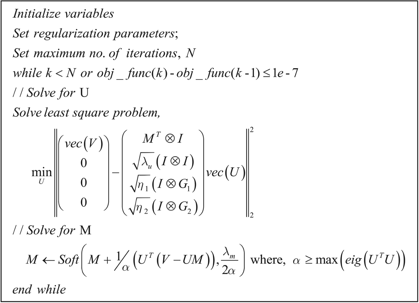
 $$\eqalign{& V=U_k M_k +\displaystyle{{1} \over {\beta}}A^T\lpar Y-A\lpar U_k M_k \rpar \rpar \cr & \mathop{\min}\limits_U \Vert V-UM \Vert _F^2 +\lambda_u \Vert U \Vert _F^2 +\eta_1 \Vert G_1 U\Vert _F^2 \cr & \quad \quad + \eta_2 \Vert G_2 U \Vert _F^2.} $$
The minimization problem in (25) can be recast as
 $$\mathop{\min}\limits_U \left\Vert \left({\matrix{vec\lpar V\rpar \cr 0 \cr 0 \cr 0 \cr }} \right)-\left({\matrix{ M^T \otimes I \cr \sqrt{\lambda_u} \lpar I \otimes I\rpar \cr \sqrt{\eta_1} \lpar I \otimes G_1\rpar \cr \sqrt{\eta_2} \lpar I \otimes G_2\rpar \cr } }\right)vec\lpar U\rpar \right\Vert _2^2\comma \; $$
which is a simple least-squares formulation having a closed-form solution.
Now, Considering sub-problem 2 (24), we use MM scheme to break it into simpler steps
 $$\eqalign {& V=U_k M_k + 1/\beta A^T\lpar Y-A\lpar U_k M_k\rpar \rpar \cr & \mathop{\min}\limits_M \Vert V-UM\Vert _F^2 +\lambda _m \Vert vec\lpar M\rpar \Vert _1} $$
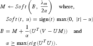
The minimization step in (27) can be solved using iterative soft thresholding [Reference Daubechies, Defrise and Mol30] as follows:
 $$\eqalign{ & M \leftarrow Soft \left(B\comma \; \displaystyle{{\lambda_m} \over {2\alpha}}\right)\quad \hbox{where}\comma \; \cr & \quad Soft\lpar t\comma \; u\rpar =\hbox{sign}\lpar t\rpar \, \max \lpar 0\comma \; \vert t \vert -u\rpar \cr & B=M+\displaystyle{{1} \over {\alpha}}\lpar U^T\lpar V-UM\rpar \rpar \quad \hbox{and} \cr & \quad \alpha \ge \max \lpar eig\lpar U^TU\rpar \rpar .} $$
Both the sub-problems are alternately solved until convergence, i.e. either the maximum number of iterations reached or reduction in objective function falls below the threshold over consecutive iterations. The complete algorithm (BCS-User-Metadata) is given in Fig. 1.

Fig. 1. Algorithm for BCS-User-Metadata.
2) Algorithm – item metadata in the BCS framework
In this section, we discuss our algorithm using MM for our formulation proposed in (18) repeated here for convenience involving item metadata.
Similar to the procedure followed above, we use ADMM to split the problem into simpler sub-problems
Sub-problem 2
First, considering sub-problem 1, using MM we can write it as iterative steps
 $$\eqalign{ & V=U_k M_k +\displaystyle{{1} \over {\beta}} A^T\lpar Y-A\lpar U_k M_k\rpar \rpar \cr & \mathop{\min}\limits_U \Vert V-UM\Vert _F^2 +\lambda_u \Vert U \Vert _F^2.} $$
Equation (32) can be recast into simple least-squares form (33) having the closed-form solution
 $$\mathop{\min}\limits_U \left\Vert \left({\matrix{ V \cr 0 \cr}}\right)-U\left({\matrix{ M \cr \sqrt{\lambda_u} I \cr }} \right)\right\Vert _2^2. $$
Now, moving to sub-problem 2, we consider each group separately, i.e. one group at a time. Applying the MM technique we can rewrite the same (for say group 1) as
 $$\eqalign{ V & = U_k M_k +\displaystyle{{1} \over {\beta}}A^T\lpar Y-A\lpar U_k M_k \rpar \rpar \cr & \quad \times \mathop{\min}\limits_M \Vert V_1 -UM_1 \Vert _F^2 +\lambda_m \Vert M_1\Vert _{2\comma 1}\comma \; } $$
where V 1 is the set of columns of V having correspondence in M 1.
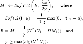
Solution to minimization problem in (34) is given by [Reference Chartrand and Wohlberg31]
 $$\eqalign{ & M_1 \leftarrow SofT\_2\left(B\comma \; \displaystyle{{\lambda_m} \over {2\gamma}}\right)\comma \; \quad \hbox{where} \cr & \quad Soft\_2 \lpar {\bf t}\comma \; u\rpar =\displaystyle{{\bf t} \over {\Vert {\bf t}\Vert _2}} \max\lpar 0\comma \; \Vert {\bf t} \Vert_2 -u\rpar \comma \; \cr & B=M_1 +\displaystyle{{1} \over {\gamma }}\lpar U^T\lpar V_1 -UM_1 \rpar \rpar \quad \hbox{and} \cr & \quad \gamma \ge \max\lpar eig\lpar U^TU\rpar \rpar .} $$
Similar procedure is repeated for all groups (formed as per genre data). The overall item's latent factor vector is computed as an average of latent factor vectors obtained from each group data. The two sub-problems are alternately solved until convergence. The complete algorithm (BCS-Item-Metadata) is given in Fig. 2.

Fig. 2. Algorithm for BCS-Item-Metadata.
IV. EXPERIMENTAL SETUP AND RESULTS
We conducted experiment on 100 K and 1 M datasets in the movielens repository (http://grouplens.org/datasets/ movielens/). These datasets from Grouplens are the most widely used publically available datasets for evaluating the performance of RSs. Both datasets contain user (demography) and item (category) metadata apart from the explicit rating data. The larger (10 million) dataset from the Movielens repository contains only the explicit rating values and no associated metadata and hence, our evaluation is restricted to 100 K and 1 M datasets. We are not aware of other datasets that provide the required metadata.
We compared our results with existing state of the art methods for MF and works incorporating similar metadata information.
A) Description of dataset
The 100 K dataset consists of 100 000 ratings (on a scale of 1–5) given by 943 users on a total of 1682 movies. The 1 M dataset has about 3900 movie ids, 6040 users, and 1 million ratings. Both the datasets are extremely sparse (<5% of ratings available) and hence an optimum candidate for illustrating the benefits of adding metadata toward improving prediction accuracy.
For incorporating user metadata (for both datasets) we consider their age–gender combination and occupational profiles. For 100 K dataset, the groups formed are Male and Female in age brackets of 1–10, 11–20, 21–30, 31–40, 41–50, 51–60, 61–70, and 71–80. Thus, we have a total of 18 groups of similar users as per their age–gender combination. We also grouped users on the basis of their occupation, wherein there are 21 different occupations and equal number of groups. In case of 1 M dataset, there are seven different age groups: 1–17, 18–24, 25–34, 35–44, 45–49, 50–55, and 56+. So, a total of 14 groups are made with age–gender (M/F) information. Similar to 100 K dataset, users are divided into 21 groups based on their occupation.
Item metadata is exploited by forming 19 groups as per the available genre information in case of both the datasets. Each movie can belong to more than one genre and hence the groups are overlapping.
B) Parameter selection and evaluation criteria
We performed fivefold cross-validation on both the datasets with 80% data forming the train set and remaining 20% used as test data. For each algorithm–test set combinations, 100 independent simulations were carried out and the results show are the mean values and standard deviation for all 100 runs. The simulations are carried out on system with i7–3770S CPU at 3.10 | GHz with 8 | GB RAM.
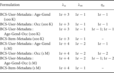
We computed the baseline offline using (3) with regularization parameter kept at 1e–3. For BCS algorithm we used the code provided by authors of [Reference Lingala and Jacob25]. The parameter selection for our formulations was done using L-curve technique [Reference Lawson and Hanson32]. The values for all the formulations namely, BCS-User-Metadata (16) for cases using only age–gender information, only occupational data and both combined together and BCS-Item-Metadata (18) are given in Table 1.
Table 1. Regularization parameter values.

The performance of the proposed approach viz-a-viz other methods is evaluated on the basis of two error measures – mean absolute error (MAE) (37) and root-mean-square error (RMSE) (38), where R contains the actual rating values, ![]() $\hat{R}$ consists of predicted ratings, and | R| is the cardinality of the rating matrix.
$\hat{R}$ consists of predicted ratings, and | R| is the cardinality of the rating matrix.
 $$\hbox{MAE} = \displaystyle{{\sum\limits_{u\comma m} R_{u\comma m}-\hat{R}_{u\comma m}} \over {\vert R \vert }}\comma \; $$
 $$\hbox{RMSE} = \sqrt{\displaystyle{{\sum\limits_{u\comma m} \lpar R_{u\comma m} -\hat{R}_{u\comma m}\rpar ^2} \over {\vert R \vert }}}. $$
In addition to these error measures, we also evaluate the performance of algorithms in terms of top-N recommendation accuracy via precision (38) and recall (39) [Reference Shani, Gunawardana, Ricci, Rokach, Shapira and Kantor33].
where t p denotes the true positive (item relevant and recommended), f p denotes the false positive (item irrelevant and recommended), and f n denotes the false negative (item relevant and not recommended). To differentiate the relevant and irrelevant items, we binarize the available ratings; marking the items rated as 4 or 5 as irrelevant, and those rated below (1–3) as irrelevant to the user. We plot the precision and recall curves for varying number of recommendations (N) for all algorithms.
C) Performance evaluation of novel MF (BCS) formulation
In this section, we highlight the improvement in prediction accuracy achieved by use of our modified MF model, i.e. BCS framework (12). We compare the performance of our formulation – BCS algorithm – against the state-of-the-art MF algorithms, namely, SGD [Reference Koren, Bell and Volinsky14], PMF [Reference Mnih, Salakhutdinov, Platt, Koller, Singer and Roweis15] and Block co-ordinate descent algorithm for non-negative matrix factorization (BCD-NMF) [Reference Xu and Yin16]. SGD algorithm involves online baseline estimation, whereas the other two work with raw (non-negative) rating data. For our formulation, BCS, baseline correction is carried out offline.
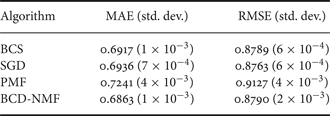
Table 2 lists the MAE and RMSE values for all the algorithms for 100 K dataset. The error values for our formulation and SGD is about 2% better than those for the other two algorithm (PMF and BCD-NMF), highlighting the importance of baseline estimation. Despite the online baseline estimation carried out in the SGD algorithm, our formulation gives an improvement of over 1% in the MAE value as compared with the former. Table 3 gives similar values for the 1 M dataset. Here also, it can be observed that the methods involving baseline estimation give superior results. For 1M dataset also, our algorithm gives the highest prediction accuracy among the algorithms compared.
Table 2. Error measures (100 K dataset).

Table 3. Error measures (1 M dataset).

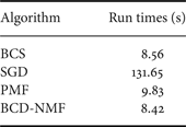
Table 4 gives the run time comparison for various algorithms compared above for 100 K dataset. It can be seen from values in the table that our novel BCS formulation performs comparable in terms of run time to existing state-of-the-art methods while providing substantial gain in terms of recovery accuracy.
Table 4. Run time comparison (100 K dataset).
Figures 3 and 4 give the precision and recall values as a function of number of recommendations for all the algorithms compared above for the 100 K dataset. Corresponding graph for 1M dataset are shown in Figs 5 and 6. Our formulation (BCS) performs better (especially for 1M dataset) or comparable with other state-of-the-art methods on this measure as well.

Fig. 3. Precision (100 K).

Fig. 4. Recall (100 K).

Fig. 5. Precision (1 M).

Fig. 6. Recall (1 M).
The above results validate our claim that our formulation promoting recovery of a dense user and sparse item latent factor matrix better models the rating data.
D) Effect of incorporating user and item metadata
In this section, we demonstrate the impact of incorporating user and item metadata to our BCS formulation. We study the impact of user metadata (age–gender, occupation, and both combined) and item metadata (genre information) on prediction accuracy. We compare the result of our formulations incorporating metadata – BCS-User-Metadata (16) and BCS-Item-Metadata (18) with those obtained using the base BCS framework.
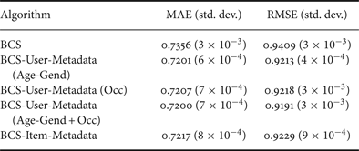
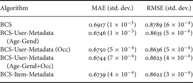
Tables 5 and 6 list the MAE and RMSE values for all the formulations for 100 K and 1 M datasets, respectively. Use of metadata to supplement the rating data using our formulation is able to bring an improvement of over 2% in prediction accuracy (in terms of MAE values) over the BCS formulation using only rating data, which is a substantial gain. Among the metadata information, grouping using user demographic data give slightly better results than the item category information. Further, age–gender-based grouping is able to capture the user similarity better and additional use of occupational profile does not introduce any substantial improvement. For the 1 M dataset, the improvement is around even more pronounced (>2.5%). This is because the rating matrix for 1 M dataset is ever sparser and hence better benefits from use of secondary data.
Table 5. Error measures (100 K dataset).

Table 6. Error measures (1 M dataset).

Figures 7 and 8 give the precision and recall values all the algorithms for 100 K dataset and Figs 9 and 10 gives similar graphs for 1M dataset. It can be observed from the figure that inclusion of metadata in the model helps improve both precision and recall considerably. For each item or user metadata, the values are almost comparable.

Fig. 7. Precision (100 K).

Fig. 8. Recall (100 K).

Fig. 9. Precision (1 M).

Fig. 10. Recall (1 M).
E) Comparison with existing methods
This section contains the comparison of our proposed formulations (BCS-User-Metadata and BCS-Item-Metadata) with existing works exploiting user/item metadata. We also show the results for combine formulation using both item and user metadata (BCS-User-Item-Metadata) (19). We compare our work with graph-regularized matrix factorization (Graph-Reg NMF) formulation proposed in [Reference Gu, Zhou and Ding20] and the neighborhood method (KNN-based) proposed in [Reference Vozalis and Margaritis18], both utilizing user's auxiliary (demographic) information. These two works are representative of the existing state-of-the-art formulation incorporating metadata information; others rely on social profiling and network information.
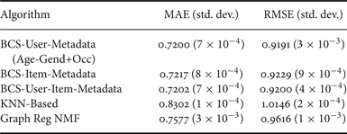
Tables 7 and 8 give the MAE and RMSE values for 100 K and 1 M datasets, respectively. The values clearly indicate the superiority of our design over the neighborhood based as well as latent factor model. The prediction accuracy is lowest for neighborhood-based methods showing the advantage of latent factor models in better modeling the rating data. Our algorithm is able to achieve about 5% better MAE than the graph-Reg NMF algorithm for the 100 K dataset.
Table 7. Error measures (100 K dataset).

Table 8. Error measures (1 M dataset).

The improvement for 1 M dataset is even higher about 7.5% for MAE values. Use of user's demographic data gives slightly better results than item category information. However, combining item information with user data does not increase the prediction accuracy further.
As can be observed from the values in Tables 5–8, that use of user or item metadata with the rating information provide considerable improvement in prediction accuracy. However, a combination of user and item metadata together with rating information is unable to surpass the performance of algorithms using either of the metadata. This observation can be explained by going back to latent factor model's assumption of interaction between users and items. As per the latent factor model, only a few factors determine a user's choice of an item. Thus, there exists correlation among users and items which is reflected in the low-rank nature of the rating matrix. The rating data is highly sparse and thus unable to capture the interaction between users and items completely. Use of either user or item metadata helps provide additional data to establish this correlation further. However, there is a practical limit to which such metadata or item–user correlation can be exploited to improve accuracy. Sufficient information is captured by rating and user or item metadata to provide further benefit of additional metadata. Also, the formulation suffer from practical implementation constraint in terms of selecting optimal regulation parameters and others which hinders further improvement in accuracy.
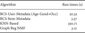
Table 9 gives the run time comparison of our formulation using user metadata and item genre information with existing works. Here also, our formulation utilizing item metadata has run times comparable with state-of-the-art methods while achieving a significant reduction in error measures. Even though our user metadata-based formulation has higher run times than the Graph-Reg method, it is still reasonable and far lesser than neighborhood-based scheme. Also, the improvement in prediction accuracy compensates for run time increase.
Table 9. Run time comparison (100 K dataset).
Figures 11 and 12 give the precision and recall values for 100 K dataset. Our algorithm outperforms the other two approaches by a wide margin on this measure. Figures 13 and 14 show the same data curves for 1 M dataset. Here also, our algorithm performs better or comparably to others. The item and user metadata based formulations based on BCS, both perform comparably.

Fig. 11. Precision (100 K).

Fig. 12. Recall (100 K).

Fig. 13. Precision (1 M).

Fig. 14. Recall (1 M).
V. CONCLUSION
In this work, we propose to improve the accuracy of rating prediction in RSs by the twofold method. Firstly, we propose a novel formulation based on latent factor model for collaborative filtering. The basic formulation remains the same, i.e. the ratings matrix can be factored into two matrices – user latent factor matrix and item latent factor matrix. However, all prior studies assumed that both these matrices are dense. We argue that this is not the case; the user latent factor matrix is dense, but the item latent factor matrix is supposed to be sparse. This is because all users are likely to have an affinity for all the different factors, but it is not possible for the items to possess all factors simultaneously. We show that our proposed formulation naturally fits into the recently proposed BCS framework.
Next we proposed a model to include user and item metadata into the BCS framework to alleviate the problem of data sparsity. Our model is based on the assumption that users sharing similar demographic profiles tend to show similar affinities toward various features (latent factors). Thus, we attempt to minimize the variance among latent factor vectors of such similar users. Also, we argue that items which belong to common genre have structurally similar latent factor vectors, i.e. they have common sparsity pattern. We exploit these beliefs to include metadata into our BCS framework. Most existing works focus on using social information which is not very readily information. We use user demographic data and item categories which are more widely and easily obtainable, making our model more feasible. As BCS is a recent framework and there are no efficient algorithms for solving the same, we also propose efficient algorithms for our formulations using MM technique.
In the future, we would like to extend our design for other RS examples as well such as books or restaurants.
Anupiya Gogna has been a Research Scholar at Indraprastha Institute of Information Technology, Delhi since July 2013. She completed her M. Tech (ECE) from Indira Gandhi Institute of Technology, Delhi in 2012. Her research interest includes signal processing, metaheuristics, compressive sensing, and sparse signal recovery with focus on matrix factorization and collaborative filtering algorithms. She has authored several research papers in reputed journals and conferences.
Angshul Majumdar has been an Assistant Professor at Indraprastha Institute of Information Technology, Delhi since October 2012. He completed his Ph.D. from the University of British Columbia in 2012. His research focuses on algorithms and applications of sparse signal recovery and low-rank matrix recovery; his works on a wide range of topics, including biomedical signal and image processing, remote sensing, data analytics, and machine learning. He has written over 100 journal and conference papers since the inception of his research career in 2007. He has recently published a book on Compressed Sensing-based MRI Reconstruction with Cambridge University Press.


