


1. Introduction
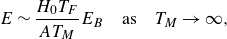
The hydrodynamic pilot-wave system (Bush Reference Bush2010), discovered in 2005 by Yves Couder and Emmanuel Fort (Couder et al. Reference Couder, Fort, Gautier and Boudaoud2005a ) has garnered considerable interest owing to its relation to quantum systems (Couder et al. Reference Couder, Protière, Fort and Boudaoud2005b ), and has provided the basis for the field of hydrodynamic quantum analogues (Bush & Oza Reference Bush and Oza2021). The system consists of a millimetric droplet bouncing on the surface of a vibrating liquid bath. The vibrational acceleration is always less than the Faraday threshold (Benjamin & Ursell Reference Benjamin and Ursell1954; Kumar & Tuckerman Reference Kumar and Tuckerman1994; Kumar Reference Kumar1996), above which Faraday waves arise even in the absence of the droplet, so the wave field navigated by the droplet is always entirely of its own making. The control parameter of the system is the bath’s vibrational acceleration, which prescribes the longevity of the waves generated by the droplet impacts, and so the ‘memory’ of the system (Eddi et al. Reference Eddi, Sultan, Moukhtar, Fort, Rossi and Couder2011). Increasing the memory progressively towards the Faraday threshold prompts the stationary bouncing droplet to destabilise into a ‘walker’, a macroscopic realisation of wave–particle duality consisting of a self-propelling droplet dressed in a quasi-monochromatic pilot-wave form (Bush Reference Bush2015; Bush & Oza Reference Bush and Oza2021). As the memory is further increased, the walking speed and spatial extent of the wave field increase, while the droplet moves downwards on its pilot wave, towards a region with higher slope (see figure 1).

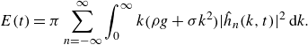
Figure 1. Stroboscopic pilot-wave fields,
 $h({\boldsymbol{x}},t)$
, generated by
$h({\boldsymbol{x}},t)$
, generated by
 $(a)$
a stationary bouncer and
$(a)$
a stationary bouncer and
 $(b,c)$
walkers for vibrational forcing (a)
$(b,c)$
walkers for vibrational forcing (a)
 $\gamma = \gamma _W$
(the walking threshold), (b)
$\gamma = \gamma _W$
(the walking threshold), (b)
 $\gamma /\gamma _F = 0.9$
and (c)
$\gamma /\gamma _F = 0.9$
and (c)
 $\gamma /\gamma _F = 0.97$
. Upper panels: overhead view of the stroboscopic wave field accompanying the droplet, with regions of elevation and depression highlighted in red and blue, respectively. Lower panels: the wave profile (in μm) along the line of droplet motion. The droplet speed and wave energy increase with the vibrational forcing, with the wave field spanning the plane in the high-memory limit. As the droplet moves faster, it moves away from the wave crest towards a region with higher slope, inducing a corresponding decrease in the local wave elevation. The plots are generated by solving the stroboscopic pilot-wave model (2.1) for walking at a constant speed (see (4.3)) with physical parameters
$\gamma /\gamma _F = 0.97$
. Upper panels: overhead view of the stroboscopic wave field accompanying the droplet, with regions of elevation and depression highlighted in red and blue, respectively. Lower panels: the wave profile (in μm) along the line of droplet motion. The droplet speed and wave energy increase with the vibrational forcing, with the wave field spanning the plane in the high-memory limit. As the droplet moves faster, it moves away from the wave crest towards a region with higher slope, inducing a corresponding decrease in the local wave elevation. The plots are generated by solving the stroboscopic pilot-wave model (2.1) for walking at a constant speed (see (4.3)) with physical parameters
 $f = 80$
Hz,
$f = 80$
Hz,
 $\rho = 950 \mbox { kg m}^{-3}$
,
$\rho = 950 \mbox { kg m}^{-3}$
,
 $\nu = 20.9$
cSt,
$\nu = 20.9$
cSt,
 $\sigma = 0.206 \mbox { N m}^{-1}$
,
$\sigma = 0.206 \mbox { N m}^{-1}$
,
 $\mathcal {H} = 4$
mm,
$\mathcal {H} = 4$
mm,
 $R =$
0.4 mm,
$R =$
0.4 mm,
 $\sin \varPhi = 0.2$
, and
$\sin \varPhi = 0.2$
, and
 $T_d = 0.0174$
s (see table 1). The walking threshold is
$T_d = 0.0174$
s (see table 1). The walking threshold is
 $\gamma _W/\gamma _F = 0.782$
, the Faraday wavelength is
$\gamma _W/\gamma _F = 0.782$
, the Faraday wavelength is
 $\lambda _F = 4.75$
mm and the maximum steady walking speed is
$\lambda _F = 4.75$
mm and the maximum steady walking speed is
 $c = 13.3 \mbox { mm s}^{-1}$
.
$c = 13.3 \mbox { mm s}^{-1}$
.
The hydrodynamic pilot-wave system is driven and dissipative (Kutz et al. Reference Kutz, Rahman, Ebers, Koch and Bramburger2022; Rahman & Kutz Reference Rahman and Kutz2023); specifically, energy is fed into the system through the bath vibration and dissipated through the action of fluid viscosity. This dissipation ultimately leads to a warming of the bath and an associated drift of the Faraday threshold (Douady Reference Douady1990; Harris et al. Reference Harris, Moukhtar, Fort, Couder and Bush2013; Ellegaard & Levinsen Reference Ellegaard and Levinsen2020). Nevertheless, a number of steady, periodic and statistically steady dynamical states may be achieved in which the driving and dissipation effectively balance over the time scales of interest (seconds or minutes), so that the global energetics need not be considered. Examples include steady walking states and orbital motion when the droplet moves in response to an external force field (Fort et al. Reference Fort, Eddi, Boudaoud, Moukhtar and Couder2010; Harris & Bush Reference Harris and Bush2014; Perrard et al. Reference Perrard, Labousse, Miskin, Fort and Couder2014b ). The existence and stability of the system’s various dynamical states change with the vibrational forcing, which in turn prescribes the spatial extent and longevity of the wave field. In the high-memory limit, the pilot-wave dynamics often appears chaotic (Tambasco et al. Reference Tambasco, Harris, Oza, Rosales and Bush2016), with the droplet motion intermittently switching between weakly unstable periodic states (Harris & Bush Reference Harris and Bush2014; Perrard et al. Reference Perrard, Labousse, Fort and Couder2014a ). A number of connections have been made between the energy of different dynamical states and their relative stability. For example, stable steady walking, orbiting and periodic states are all energetically favourable relative to unstable stationary bouncing (Durey & Milewski Reference Durey and Milewski2017; Durey et al. Reference Durey, Milewski and Bush2018; Liu et al. Reference Liu, Durey and Bush2023). Energetic considerations also arise in bound states formed from multiple droplets. For example, the wave energy of promenading pairs (Arbelaiz et al. Reference Arbelaiz, Oza and Bush2018), consisting of two coupled droplets walking in tandem, is less than that of two free walkers (Borghesi et al. Reference Borghesi, Moukhtar, Labousse, Eddi, Fort and Couder2014; Durey & Milewski Reference Durey and Milewski2017). Finally, rings of bouncing droplets destabilise and execute a number of discrete rearrangements in such a way as to minimise their net gravitational potential energy (Couchman & Bush Reference Couchman and Bush2020; Thomson et al. Reference Thomson, Durey and Rosales2020b ).
Despite the growing number of connections between energy and stability, a global account of the energy evolution of the pilot-wave system has not been forthcoming. One recent advancement, however, was made by Liu et al. (Reference Liu, Durey and Bush2023), who demonstrated that for droplets executing circular orbits, the wave energy and the droplet gravitational potential energies are both prescribed by the droplet speed. Through systematic analysis of the system energetics, we here demonstrate the generality of this result by deriving a speed-dependent energy diminution factor relating the wave energy and drop gravitational potential energy of dynamic states to those of the static bouncing state. Our results are valid for a number of canonical settings, including steady and quasi-steady dynamics, periodic and slow oscillatory dynamics and statistically steady states.
In § 2, we introduce the pilot-wave system and determine evolution equations for the wave and droplet energies. We utilise these results in § 3 to determine the dependence of energy on the droplet’s speed for canonical dynamical and statistically steady states. A number of illustrative numerical examples are presented in § 4. In § 5, we enumerate insights into pilot-wave hydrodynamics provided by our energetic analysis.
Table 1. Table of parameters defining the stroboscopic pilot-wave model (Moláček & Bush Reference Moláček and Bush2013a ,Reference Moláček and Bush b ; Oza et al. Reference Oza, Rosales and Bush2013).

2. Pilot-wave hydrodynamics
We consider a vertically vibrating liquid with periodic acceleration
 $\gamma \sin (2\pi f t)$
at time
$\gamma \sin (2\pi f t)$
at time
 $t$
. All relevant parameters are defined in table 1. For
$t$
. All relevant parameters are defined in table 1. For
 $\gamma \gt \gamma _F$
, the fluid rest state destabilises to a field of subharmonic standing or Faraday waves, with wavelength
$\gamma \gt \gamma _F$
, the fluid rest state destabilises to a field of subharmonic standing or Faraday waves, with wavelength
 $\lambda _F = 2\pi /k_F$
and period
$\lambda _F = 2\pi /k_F$
and period
 $T_F = 2/f$
. Below the Faraday threshold,
$T_F = 2/f$
. Below the Faraday threshold,
 $\gamma \lt \gamma _F$
, any waves generated at the free surface, for example by a bouncing droplet, are subcritical, decaying over a time scale,
$\gamma \lt \gamma _F$
, any waves generated at the free surface, for example by a bouncing droplet, are subcritical, decaying over a time scale,
 $T_M$
, that increases with proximity to the Faraday threshold. For the weakly viscous liquids used in experiments (Wind-Willassen et al. Reference Wind-Willassen, Moláček, Harris and Bush2013), the Faraday wavenumber,
$T_M$
, that increases with proximity to the Faraday threshold. For the weakly viscous liquids used in experiments (Wind-Willassen et al. Reference Wind-Willassen, Moláček, Harris and Bush2013), the Faraday wavenumber,
 $k_F$
, approximately satisfies the gravity–capillary dispersion relation,
$k_F$
, approximately satisfies the gravity–capillary dispersion relation,
 $(\pi f)^2 = (g k_F + \sigma k_F^3/\rho)\tanh (k_F \mathcal {H})$
(Benjamin & Ursell Reference Benjamin and Ursell1954).
$(\pi f)^2 = (g k_F + \sigma k_F^3/\rho)\tanh (k_F \mathcal {H})$
(Benjamin & Ursell Reference Benjamin and Ursell1954).
2.1. Governing equations
We model the evolution of a resonant walker bouncing with period
 $T_F$
, in perfect synchrony with its subharmonic pilot wave,
$T_F$
, in perfect synchrony with its subharmonic pilot wave,
 $\eta ({\boldsymbol{x}},t)$
. We thus assume that each drop impact arises at the same wave amplitude and phase, the basis of the stroboscopic approximation (Oza et al. Reference Oza, Rosales and Bush2013). The droplet is propelled by the wave force
$\eta ({\boldsymbol{x}},t)$
. We thus assume that each drop impact arises at the same wave amplitude and phase, the basis of the stroboscopic approximation (Oza et al. Reference Oza, Rosales and Bush2013). The droplet is propelled by the wave force
 $\boldsymbol{F\!}_w(t) = -F(t) \nabla \eta ({\boldsymbol{x}}_{{\kern-1.5pt}p},t)$
and resisted by drag, where
$\boldsymbol{F\!}_w(t) = -F(t) \nabla \eta ({\boldsymbol{x}}_{{\kern-1.5pt}p},t)$
and resisted by drag, where
 ${\boldsymbol{x}}_{{\kern-1.5pt}p}(t)$
denotes the droplet’s horizontal position at time
${\boldsymbol{x}}_{{\kern-1.5pt}p}(t)$
denotes the droplet’s horizontal position at time
 $t$
and
$t$
and
 $F(t)$
is the periodic vertical force acting on the droplet. Notably, the vertical force averaged over one bouncing period,
$F(t)$
is the periodic vertical force acting on the droplet. Notably, the vertical force averaged over one bouncing period,
 $T_F$
, is precisely equal to the droplet weight, namely
$T_F$
, is precisely equal to the droplet weight, namely
 $\overline {F(t)} = mg$
. As the time scale of the droplet’s horizontal motion greatly exceeds that of its vertical motion, we model the wave field as
$\overline {F(t)} = mg$
. As the time scale of the droplet’s horizontal motion greatly exceeds that of its vertical motion, we model the wave field as
 $\eta ({\boldsymbol{x}},t) = \cos (\pi f t) \bar \eta ({\boldsymbol{x}},t)$
, representing the superposition of a fast subharmonic oscillation modulated by a slowly varying spatial profile (Moláček & Bush Reference Moláček and Bush2013b
). Time-averaging the droplet wave force over one bouncing period thus yields
$\eta ({\boldsymbol{x}},t) = \cos (\pi f t) \bar \eta ({\boldsymbol{x}},t)$
, representing the superposition of a fast subharmonic oscillation modulated by a slowly varying spatial profile (Moláček & Bush Reference Moláček and Bush2013b
). Time-averaging the droplet wave force over one bouncing period thus yields
 $\overline {\boldsymbol{F\!}_w(t)} = -mg\nabla h({\boldsymbol{x}}_{{\kern-1.5pt}p},t)$
, where
$\overline {\boldsymbol{F\!}_w(t)} = -mg\nabla h({\boldsymbol{x}}_{{\kern-1.5pt}p},t)$
, where
 $h({\boldsymbol{x}},t) = \mathscr {C}\, \bar \eta ({\boldsymbol{x}},t)$
is the stroboscopic wave field and
$h({\boldsymbol{x}},t) = \mathscr {C}\, \bar \eta ({\boldsymbol{x}},t)$
is the stroboscopic wave field and
 $\mathscr {C} = \overline {F(t)\cos (\pi f t)}/mg$
denotes the phase of droplet impact relative to the wave-field oscillation (Moláček & Bush Reference Moláček and Bush2013b
; Couchman et al. Reference Couchman, Turton and Bush2019). The time-averaged horizontal force balance may then be written as (Moláček & Bush Reference Moláček and Bush2013b
)
$\mathscr {C} = \overline {F(t)\cos (\pi f t)}/mg$
denotes the phase of droplet impact relative to the wave-field oscillation (Moláček & Bush Reference Moláček and Bush2013b
; Couchman et al. Reference Couchman, Turton and Bush2019). The time-averaged horizontal force balance may then be written as (Moláček & Bush Reference Moláček and Bush2013b
)
 \begin{equation} m \ddot{\boldsymbol{x}}_{{\kern-1.5pt}p} + D \dot{\boldsymbol{x}}_{{\kern-1.5pt}p} = -mg \nabla h ({\boldsymbol{x}}_{{\kern-1.5pt}p}, t) + \boldsymbol{F}, \end{equation}
where
 $\boldsymbol{F}$
is an applied force and dots denote derivatives with respect to time.
$\boldsymbol{F}$
is an applied force and dots denote derivatives with respect to time.
We model the stroboscopic pilot wave by the integral
 \begin{equation} h({\boldsymbol{x}},t) = \frac {A}{T_F} \int _{-\infty }^t \mathscr {H}\ (|{\boldsymbol{x}} - {\boldsymbol{x}}_{{\kern-1.5pt}p}(s)|)\mathrm {e}^{-(t - s)/T_M}{\, \mathrm {d}s}, \end{equation}
which represents a superposition of axisymmetric quasi-monochromatic waves of amplitude
 $A$
centred along the droplet’s path and decaying over the memory time scale,
$A$
centred along the droplet’s path and decaying over the memory time scale,
 $T_M$
(Oza et al. Reference Oza, Rosales and Bush2013). Experimentally, this represents the wave form observed when the system is strobed at the Faraday frequency, and images captured at the phase of droplet impact, so that the droplet appears to surf along its pilot wave. The system (2.1) represents the stroboscopic model (Oza et al. Reference Oza, Rosales and Bush2013) of pilot-wave hydrodynamics, which has proven to be adequate in rationalising the bulk of observed walker behaviours (Oza et al. Reference Oza, Harris, Rosales and Bush2014a
; Turton et al. Reference Turton, Couchman and Bush2018). Nevertheless, it is known to have shortcomings when non-resonant effects arise (Primkulov et al. Reference Primkulov, Evans, Been and Bush2025), specifically when the walker bouncing phase varies owing to variability in the local wave form (Harris et al. Reference Harris, Moukhtar, Fort, Couder and Bush2013; Durey et al. Reference Durey, Milewski and Wang2020), which is particularly prevalent at high memory (Moláček & Bush Reference Moláček and Bush2013b
; Wind-Willassen et al. Reference Wind-Willassen, Moláček, Harris and Bush2013). Consequently, the results of our study are unlikely to be applicable in experiments close to the Faraday threshold, for which exotic and chaotic bouncing modes (Protière et al. Reference Protière, Boudaoud and Couder2006; Wind-Willassen et al. Reference Wind-Willassen, Moláček, Harris and Bush2013) are expected to significantly alter the pilot-wave energetics.
$T_M$
(Oza et al. Reference Oza, Rosales and Bush2013). Experimentally, this represents the wave form observed when the system is strobed at the Faraday frequency, and images captured at the phase of droplet impact, so that the droplet appears to surf along its pilot wave. The system (2.1) represents the stroboscopic model (Oza et al. Reference Oza, Rosales and Bush2013) of pilot-wave hydrodynamics, which has proven to be adequate in rationalising the bulk of observed walker behaviours (Oza et al. Reference Oza, Harris, Rosales and Bush2014a
; Turton et al. Reference Turton, Couchman and Bush2018). Nevertheless, it is known to have shortcomings when non-resonant effects arise (Primkulov et al. Reference Primkulov, Evans, Been and Bush2025), specifically when the walker bouncing phase varies owing to variability in the local wave form (Harris et al. Reference Harris, Moukhtar, Fort, Couder and Bush2013; Durey et al. Reference Durey, Milewski and Wang2020), which is particularly prevalent at high memory (Moláček & Bush Reference Moláček and Bush2013b
; Wind-Willassen et al. Reference Wind-Willassen, Moláček, Harris and Bush2013). Consequently, the results of our study are unlikely to be applicable in experiments close to the Faraday threshold, for which exotic and chaotic bouncing modes (Protière et al. Reference Protière, Boudaoud and Couder2006; Wind-Willassen et al. Reference Wind-Willassen, Moláček, Harris and Bush2013) are expected to significantly alter the pilot-wave energetics.
For the sake of simplicity, we proceed by focusing on the case of resonant walkers, and so neglect temporal variations in the droplet impact phase. We may thus treat the wave amplitude,
 $A$
, as a constant. We further assume that the wave kernel,
$A$
, as a constant. We further assume that the wave kernel,
 $\mathscr {H}\ (r)$
, is a differentiable function, with
$\mathscr {H}\ (r)$
, is a differentiable function, with
 $\mathscr {H}\ (0) = 1$
and
$\mathscr {H}\ (0) = 1$
and
 $\mathscr {H}\ (r) \lt 1$
for all
$\mathscr {H}\ (r) \lt 1$
for all
 $r \gt 0$
. Furthermore, we posit that the spectrum is localised about
$r \gt 0$
. Furthermore, we posit that the spectrum is localised about
 $k_F$
, giving rise to a quasi-monochromatic form with wavelength
$k_F$
, giving rise to a quasi-monochromatic form with wavelength
 $\lambda _F$
and exponential spatial decay in the farfield over the length scale
$\lambda _F$
and exponential spatial decay in the farfield over the length scale
 $l_d$
. Motivated by the results of prior studies (Tadrist et al. Reference Tadrist, Shim, Gilet and Schlagheck2018; Couchman et al. Reference Couchman, Turton and Bush2019), we assume that
$l_d$
. Motivated by the results of prior studies (Tadrist et al. Reference Tadrist, Shim, Gilet and Schlagheck2018; Couchman et al. Reference Couchman, Turton and Bush2019), we assume that
 $l_d(\gamma)$
increases with the vibrational forcing, and diverges in the high-memory limit.
$l_d(\gamma)$
increases with the vibrational forcing, and diverges in the high-memory limit.
2.2. Droplet energy evolution
We proceed by describing the evolution of the droplet’s kinetic and potential energy, where we express our results in terms of the local wave height,
 $H(t) = h({\boldsymbol{x}}_{{\kern-1.5pt}p},t)$
. We first use the chain rule to write
$H(t) = h({\boldsymbol{x}}_{{\kern-1.5pt}p},t)$
. We first use the chain rule to write
 $\dot H = \partial _t h({\boldsymbol{x}}_{{\kern-1.5pt}p},t) + \dot{\boldsymbol{x}}_{{\kern-1.5pt}p} \cdot \nabla h({\boldsymbol{x}}_{{\kern-1.5pt}p},t)$
, whereupon substitution of (2.1) yields
$\dot H = \partial _t h({\boldsymbol{x}}_{{\kern-1.5pt}p},t) + \dot{\boldsymbol{x}}_{{\kern-1.5pt}p} \cdot \nabla h({\boldsymbol{x}}_{{\kern-1.5pt}p},t)$
, whereupon substitution of (2.1) yields
 \begin{equation} \dot H = \frac {A}{T_F} - \frac {H}{T_M} + \frac {1}{mg}\dot{\boldsymbol{x}}_{{\kern-1.5pt}p} \cdot \Big (\boldsymbol{F} - m \ddot {\boldsymbol{x}}_{{\kern-1.5pt}p} - D \dot {\boldsymbol{x}}_{{\kern-1.5pt}p}\Big). \end{equation}
We then rearrange to find that the droplet’s energy evolves according to
 \begin{equation} \frac {\mathrm {d} {}}{\mathrm {d} {t}}\left (\frac {1}{2}m |\dot {\boldsymbol{x}}_{{\kern-1.5pt}p}|^2 + mgH\right) = \dot{\boldsymbol{x}}_{{\kern-1.5pt}p} \cdot \boldsymbol{F} + \frac {mgA}{T_F}\left (\gamma _D(|\dot {\boldsymbol{x}}_{{\kern-1.5pt}p}|) - \frac {H}{H_B}\right), \end{equation}
where
 $H_B = AT_M/T_F$
is the amplitude of the stroboscopic wave field for a bouncer,
$H_B = AT_M/T_F$
is the amplitude of the stroboscopic wave field for a bouncer,
 \begin{equation} \gamma _D(v) = 1 - \frac {v^2}{c^2} \end{equation}
is a speed-dependent diminution factor and
 $c = \sqrt {mgA/DT_F}$
is the maximum steady walking speed of a free walker, as arises in the high-memory limit (Oza et al. Reference Oza, Rosales and Bush2013).
$c = \sqrt {mgA/DT_F}$
is the maximum steady walking speed of a free walker, as arises in the high-memory limit (Oza et al. Reference Oza, Rosales and Bush2013).
For a droplet moving in response to the gradient of an applied potential,
 $\boldsymbol{F} = -\nabla V({\boldsymbol{x}}_{{\kern-1.5pt}p})$
, we may recast (2.3) as the work equation, as prescribes the rate of change of the droplet’s total energy:
$\boldsymbol{F} = -\nabla V({\boldsymbol{x}}_{{\kern-1.5pt}p})$
, we may recast (2.3) as the work equation, as prescribes the rate of change of the droplet’s total energy:
 \begin{equation} \dot E_p = \frac {mgA}{T_F}\left (\gamma _D(|\dot{\boldsymbol{x}}_{{\kern-1.5pt}p}|) - \frac {H}{H_B}\right), \quad \mathrm {where}\quad E_p = \frac {1}{2}m|\dot{\boldsymbol{x}}_{{\kern-1.5pt}p}|^2 + V({\boldsymbol{x}}_{{\kern-1.5pt}p}) + mg H \end{equation}
is the sum of the droplet’s dimensionless kinetic and potential energies. Evidently, the droplet energy increases when
 $H/H_B \lt \gamma _D(|\dot {\boldsymbol{x}}_{{\kern-1.5pt}p}|)$
, remains constant when
$H/H_B \lt \gamma _D(|\dot {\boldsymbol{x}}_{{\kern-1.5pt}p}|)$
, remains constant when
 $H/H_B = \gamma _D(|\dot {\boldsymbol{x}}_{{\kern-1.5pt}p}|)$
and decreases otherwise. The implications of (2.5) for the system’s energy budget are discussed in Appendix A.
$H/H_B = \gamma _D(|\dot {\boldsymbol{x}}_{{\kern-1.5pt}p}|)$
and decreases otherwise. The implications of (2.5) for the system’s energy budget are discussed in Appendix A.
2.3. Wave-field energy evolution
For near-critical vibrational forcing, the evolution of the Faraday wave field,
 $\eta ({\boldsymbol{x}},t)$
, may be regarded as quasi-inviscid, characterised by an exchange between kinetic energy and a combination of gravitational potential and surface energies. We thus define the gravitational potential and surface energies for small-amplitude waves (i.e.
$\eta ({\boldsymbol{x}},t)$
, may be regarded as quasi-inviscid, characterised by an exchange between kinetic energy and a combination of gravitational potential and surface energies. We thus define the gravitational potential and surface energies for small-amplitude waves (i.e.
 $|\nabla \eta | \ll 1$
) as (Moláček & Bush Reference Moláček and Bush2013b
)
$|\nabla \eta | \ll 1$
) as (Moláček & Bush Reference Moláček and Bush2013b
)
 \begin{equation} \mathscr {E}(t) = \iint _{\mathbb {R}^2} \frac {\rho g}{2} \eta ^2({\boldsymbol{x}},t) \, \mathrm {d}{\boldsymbol{x}} + \iint _{\mathbb {R}^2} \frac {\sigma }{2}|\nabla \eta |^2\, \mathrm {d}{\boldsymbol{x}}. \end{equation}
Owing to the assumed far-field exponential decay of the wave field, the integrals in (2.6) converge, which is not the case for the widely adopted and mathematically convenient choice
 $\mathscr {H}\ (r) = \mathrm {J}_0(k_F r)$
(Liu et al. Reference Liu, Durey and Bush2023), an account of which is given in Appendix B.
$\mathscr {H}\ (r) = \mathrm {J}_0(k_F r)$
(Liu et al. Reference Liu, Durey and Bush2023), an account of which is given in Appendix B.
By substituting the relationship
 $\eta ({\boldsymbol{x}},t) = \cos (\pi f t) h({\boldsymbol{x}},t)/\mathscr {C}$
into (2.6), we deduce that the energy of the wave field when time-averaged over one Faraday period, denoted
$\eta ({\boldsymbol{x}},t) = \cos (\pi f t) h({\boldsymbol{x}},t)/\mathscr {C}$
into (2.6), we deduce that the energy of the wave field when time-averaged over one Faraday period, denoted
 $\overline {\mathscr {E}(t)}$
, is related to the energy of the stroboscopic pilot wave,
$\overline {\mathscr {E}(t)}$
, is related to the energy of the stroboscopic pilot wave,
 \begin{equation} E(t) = \iint _{\mathbb {R}^2} \frac {\rho g}{2} h^2({\boldsymbol{x}},t) \, \mathrm {d}{\boldsymbol{x}} + \iint _{\mathbb {R}^2} \frac {\sigma }{2}|\nabla h|^2\, \mathrm {d}{\boldsymbol{x}}, \end{equation}
via
 $\overline {\mathscr {E}} = \frac {1}{2}E/\mathscr {C}\,^2$
. As
$\overline {\mathscr {E}} = \frac {1}{2}E/\mathscr {C}\,^2$
. As
 $\mathscr {C}$
typically lies in the range
$\mathscr {C}$
typically lies in the range
 $0.1 \lesssim \mathscr {C}\lesssim 0.2$
for walkers (Couchman et al. Reference Couchman, Turton and Bush2019), the time-averaged wave-field energy is at least one order of magnitude larger than the energy of the stroboscopic pilot wave. Nevertheless, we leverage this proportionality relationship to derive a simple formula governing the evolution for
$0.1 \lesssim \mathscr {C}\lesssim 0.2$
for walkers (Couchman et al. Reference Couchman, Turton and Bush2019), the time-averaged wave-field energy is at least one order of magnitude larger than the energy of the stroboscopic pilot wave. Nevertheless, we leverage this proportionality relationship to derive a simple formula governing the evolution for
 $E$
, and thus
$E$
, and thus
 $\overline {\mathscr {E}}$
.
$\overline {\mathscr {E}}$
.
To proceed, we recast the stroboscopic pilot wave as
 \begin{equation} h({\boldsymbol{x}},t) = \sum _{n = -\infty }^\infty \int _0^\infty k \hat {h}_n(k,t)\varPhi _n({\boldsymbol{x}},k)\, \mathrm {d}k, \end{equation}
where
 $\varPhi _n({\boldsymbol{x}},k) = \mathrm {J}_n(kr)\mathrm {e}^{\mathrm {i} n \theta }$
denotes an orthogonal set of functions defined in plane polar coordinates,
$\varPhi _n({\boldsymbol{x}},k) = \mathrm {J}_n(kr)\mathrm {e}^{\mathrm {i} n \theta }$
denotes an orthogonal set of functions defined in plane polar coordinates,
 ${\boldsymbol{x}} = r(\cos \theta,\sin \theta)$
,
${\boldsymbol{x}} = r(\cos \theta,\sin \theta)$
,
 $\mathrm {J}_n$
is the Bessel function of the first kind of order
$\mathrm {J}_n$
is the Bessel function of the first kind of order
 $n$
,
$n$
,
 $k$
is the wavenumber and
$k$
is the wavenumber and
 $\mathrm {i}$
denotes the imaginary unit. In terms of this basis decomposition, the stroboscopic wave energy defined in (2.7) is (Moláček & Bush Reference Moláček and Bush2013b
)
$\mathrm {i}$
denotes the imaginary unit. In terms of this basis decomposition, the stroboscopic wave energy defined in (2.7) is (Moláček & Bush Reference Moláček and Bush2013b
)
 \begin{equation} E(t) = \pi \sum _{n = -\infty }^\infty \int _0^\infty k \big (\rho g + \sigma k^2\big)|\hat {h}_n(k,t)|^2 \, \mathrm {d}k. \end{equation}
Furthermore, an application of Graf’s addition theorem (Abramowitz & Stegun Reference Abramowitz and Stegun1964, 9.1.79) to (2.1b ) determines that each wave mode evolves according to
 \begin{equation} \hat {h}_n(k,t) = \frac {\hat {h}_B(k)}{T_M}\int _{ -\infty }^t \varPhi _n^*({\boldsymbol{x}}_{{\kern-1.5pt}p}(s), k)\mathrm {e}^{-(t-s)/T_M}{\, \mathrm {d}s}, \end{equation}
where
 $*$
denotes complex conjugation and
$*$
denotes complex conjugation and
 $\hat {h}_B(k) = \int _0^\infty r h_B(r) \mathrm {J}_0(kr)\, \mathrm {d}r$
is the Hankel transform of the bouncer wave field, defined as
$\hat {h}_B(k) = \int _0^\infty r h_B(r) \mathrm {J}_0(kr)\, \mathrm {d}r$
is the Hankel transform of the bouncer wave field, defined as
 $h_B(r) = H_B\mathscr {H}\ (r)$
with
$h_B(r) = H_B\mathscr {H}\ (r)$
with
 $H_B = AT_M/T_F$
.
$H_B = AT_M/T_F$
.
We now exploit the fact that the spectrum of the bouncer wave field is sharply peaked around
 $k_F$
, with
$k_F$
, with
 $\hat {h}_B(k)$
being appreciable only when
$\hat {h}_B(k)$
being appreciable only when
 $|k - k_F|l_d = O(1)$
, to determine approximate expressions for
$|k - k_F|l_d = O(1)$
, to determine approximate expressions for
 $H(t)$
and
$H(t)$
and
 $E(t)$
valid in the high-memory limit, for which
$E(t)$
valid in the high-memory limit, for which
 $l_d k_F \gg 1$
. To facilitate this analysis, we first substitute the leading-order Taylor expansion
$l_d k_F \gg 1$
. To facilitate this analysis, we first substitute the leading-order Taylor expansion
 $\varPhi _n^*({\boldsymbol{x}}_{{\kern-1.5pt}p}, k) = \varPhi _n^*({\boldsymbol{x}}_{{\kern-1.5pt}p}, k_F) + O(\Delta k)$
(where
$\varPhi _n^*({\boldsymbol{x}}_{{\kern-1.5pt}p}, k) = \varPhi _n^*({\boldsymbol{x}}_{{\kern-1.5pt}p}, k_F) + O(\Delta k)$
(where
 $\Delta k = k/k_F - 1$
) into (2.9), giving
$\Delta k = k/k_F - 1$
) into (2.9), giving
 \begin{equation} \frac {\hat {h}_n(k,t)}{\hat {h}_B(k)} = \frac {1}{T_M}\int _{-\infty }^t \varPhi _n^*({\boldsymbol{x}}_{{\kern-1.5pt}p}(s), k_F)\mathrm {e}^{-(t-s)/T_M}{\, \mathrm {d}s} + O(\Delta k) = \frac {\hat {h}_n(k_F,t)}{\hat {h}_B(k_F)} + O(\Delta k), \end{equation}
or, equivalently,
 \begin{equation} \frac {\hat {h}_n(k,t)}{\hat {h}_n(k_F,t)} = \frac {\hat {h}_B(k)}{\hat {h}_B(k_F)} + O(\Delta k). \end{equation}
This relationship demonstrates that the spectrum close to
 $k_F$
is proportional to that of the bouncer wave field, which we exploit below to approximate the local wave height,
$k_F$
is proportional to that of the bouncer wave field, which we exploit below to approximate the local wave height,
 $H(t)$
, and stroboscopic wave energy,
$H(t)$
, and stroboscopic wave energy,
 $E(t)$
.
$E(t)$
.
To approximate the local wave height,
 $H(t) = h({\boldsymbol{x}}_{{\kern-1.5pt}p},t)$
, we substitute
$H(t) = h({\boldsymbol{x}}_{{\kern-1.5pt}p},t)$
, we substitute
 $\varPhi _n({\boldsymbol{x}}_{{\kern-1.5pt}p}, k) = \varPhi _n({\boldsymbol{x}}_{{\kern-1.5pt}p}, k_F) + O(\Delta k)$
and (2.11) into (2.8a
), and then exploit the fact that the integrand is sharply peaked about
$\varPhi _n({\boldsymbol{x}}_{{\kern-1.5pt}p}, k) = \varPhi _n({\boldsymbol{x}}_{{\kern-1.5pt}p}, k_F) + O(\Delta k)$
and (2.11) into (2.8a
), and then exploit the fact that the integrand is sharply peaked about
 $k_F$
for
$k_F$
for
 $l_d k_F \gg 1$
, giving
$l_d k_F \gg 1$
, giving
 \begin{equation} H(t) = \sum _{n=-\infty }^\infty \frac {\hat {h}_n(k_F,t)}{\hat {h}_B(k_F)} \varPhi _n({\boldsymbol{x}}_{{\kern-1.5pt}p}, k_F)\int _0^\infty k \hat {h}_B(k)\, \mathrm {d}k + O\big ((k_F l_d)^{-1}\big). \end{equation}
By noting that
 $h_B(0) = \int _0^\infty k \hat {h}_B(k)\, \mathrm {d}k$
, where
$h_B(0) = \int _0^\infty k \hat {h}_B(k)\, \mathrm {d}k$
, where
 $h_B(0) = H_B$
is the amplitude of the bouncer wave field, we deduce that
$h_B(0) = H_B$
is the amplitude of the bouncer wave field, we deduce that
 \begin{equation} H(t) = H_B \sum _{n = -\infty }^\infty \frac {\hat {h}_n(k_F, t)}{\hat {h}_B(k_F)}\varPhi _n({\boldsymbol{x}}_{{\kern-1.5pt}p}(t), k_F) + O\big ((k_F l_d)^{-1}\big), \end{equation}
thereby approximating the local wave height in terms of the system’s wave modes. Likewise, we substitute (2.11) into (2.8b ), giving
 \begin{equation} E(t) = \pi \sum _{n=-\infty }^\infty \frac {|\hat {h}_n(k_F,t)|^2}{\hat {h}_B^2(k_F)}\int _0^\infty k(\rho g + \sigma k^2) \hat {h}_B^2(k)\, \mathrm {d}k + O\big ((k_F l_d)^{-1}\big), \end{equation}
where we have used that
 $\hat {h}_B(k)$
is real. This expression may be written more concisely as
$\hat {h}_B(k)$
is real. This expression may be written more concisely as
 \begin{equation} E(t) = E_B\sum _{n=-\infty }^\infty \frac {|\hat {h}_n(k_F,t)|^2}{\hat {h}_B^2(k_F)} + O\big ((k_F l_d)^{-1}\big), \end{equation}
where
 \begin{equation} E_B = \pi \int _0^\infty k (\rho g + \sigma k^2)\hat {h}_B^2(k)\, \mathrm {d}k \end{equation}
is the energy of the bouncer wave field. We thus deduce from (2.13) that
 $H$
and
$H$
and
 $E$
deviate from their respective values for a stationary bouncing droplet, denoted
$E$
deviate from their respective values for a stationary bouncing droplet, denoted
 $H_B$
and
$H_B$
and
 $E_B$
, according to a weighted sum of the wave modes with wavenumber
$E_B$
, according to a weighted sum of the wave modes with wavenumber
 $k_F$
. These approximations form the foundation for our forthcoming analysis of the energy evolution of the stroboscopic wave field.
$k_F$
. These approximations form the foundation for our forthcoming analysis of the energy evolution of the stroboscopic wave field.
To determine the evolution of
 $E(t)$
, we first differentiate (2.9) and (2.13c
) with respect to time. By neglecting higher-order connections of size
$E(t)$
, we first differentiate (2.9) and (2.13c
) with respect to time. By neglecting higher-order connections of size
 $O ((k_F l_d)^{-1})$
in the high-memory limit, corresponding to
$O ((k_F l_d)^{-1})$
in the high-memory limit, corresponding to
 $k_F l_d \gg 1$
, we deduce that
$k_F l_d \gg 1$
, we deduce that
 \begin{equation} \frac {\partial {\hat {h}_n}}{\partial {t}} = \frac {\hat {h}_B(k)}{T_M} \varPhi _n^*({\boldsymbol{x}}_{{\kern-1.5pt}p}(t), k) - \frac {\hat {h}_n}{T_M} \quad \mathrm {and}\quad \frac {\mathrm {d} {E}}{\mathrm {d} {t}} = E_B \sum _{n = -\infty }^\infty \frac {2\mathrm {Re}[\partial _t \hat {h}_n^*(k_F,t) \hat {h}_n(k_F,t)]}{\hat {h}_B^2(k_F)}, \end{equation}
respectively, where
 $\mathrm {Re}$
denotes the real part. By eliminating
$\mathrm {Re}$
denotes the real part. By eliminating
 $\partial _t \hat {h}_n^*(k_F,t)$
from the second equation and using (2.13c
), we obtain
$\partial _t \hat {h}_n^*(k_F,t)$
from the second equation and using (2.13c
), we obtain
 \begin{equation} \frac {T_M}{2}\frac {\mathrm {d} {E}}{\mathrm {d} {t}} = E_B \sum _{n = -\infty }^\infty \frac {\hat {h}_n(k_F, t)}{\hat {h}_B(k_F)} \varPhi _n({\boldsymbol{x}}_{{\kern-1.5pt}p}(t), k_F) - E. \end{equation}
Finally, we use the approximate definition for
 $H(t)$
given in (2.13a
) to deduce the leading-order evolution equation for the wave energy:
$H(t)$
given in (2.13a
) to deduce the leading-order evolution equation for the wave energy:
 \begin{equation} \frac {\mathrm {d} {E}}{\mathrm {d} {t}} = \frac {2E_B}{T_M}\left (\frac {H(t)}{H_B} - \frac {E(t)}{E_B}\right). \end{equation}
The wave energy increases when the ratio of the wave height relative to a bouncer exceeds the corresponding ratio for wave energy, and decreases otherwise. Equation (2.17) represents a powerful formula for elucidating the evolution of wave energy in pilot-wave hydrodynamics, the implications of which for the system’s energy budget are discussed in Appendix A. We proceed by considering its application in a series of canonical dynamical regimes.
3. Energy evolution for canonical pilot-wave phenomena
Although the range of dynamics observed in experiments and predicted by the stroboscopic pilot-wave model (2.1) is vast (Bush Reference Bush2015; Bush & Oza Reference Bush and Oza2021), the qualitative behaviour may often be characterised by a small number of canonical regimes. To address the evolution of energy in these canonical regimes, we analyse the evolution formulae for the droplet and wave energy, as detailed in (2.5) and (2.17), respectively. Our results shed light on the dependence of energy on the droplet speed in a number of dynamical states.
The first canonical regime describes steady pilot-wave dynamics, for which the droplet and wave energies are conserved (Kutz et al. Reference Kutz, Rahman, Ebers, Koch and Bramburger2022; Liu et al. Reference Liu, Durey and Bush2023; Rahman & Kutz Reference Rahman and Kutz2023), as is the case for walking and orbiting at a constant speed. We thus deduce from (2.5) and (2.17) the respective relationships
 \begin{equation} H/H_B = \gamma _D(|\dot{\boldsymbol{x}}_{{\kern-1.5pt}p}|) \quad \mbox {and}\quad E/E_B = H/H_B, \end{equation}
giving rise to the following expressions for the droplet and wave energies:
 \begin{equation} E_p = \frac {1}{2}m |\dot{\boldsymbol{x}}_{{\kern-1.5pt}p}|^2 + V({\boldsymbol{x}}_{{\kern-1.5pt}p}) + mgH_B \gamma _D(|\dot {\boldsymbol{x}}_{{\kern-1.5pt}p}|) \quad \mathrm {and}\quad E = E_B \gamma _D(|\dot{\boldsymbol{x}}_{{\kern-1.5pt}p}|). \end{equation}
Notably, the wave and droplet gravitational potential energies are both maximised for a stationary droplet, and decrease as the droplet walks faster and its kinetic energy increases. We thus deduce that the wave energy of a walker is always less than the wave energy of the unstable bouncer at the same vibrational forcing, providing a theoretical rationale for the observations made by Durey & Milewski (Reference Durey and Milewski2017) based on their numerical computations.
The second canonical dynamical regime is periodic droplet motion, for which the average droplet and wave energies are conserved over one periodic cycle (Kutz et al. Reference Kutz, Rahman, Ebers, Koch and Bramburger2022; Rahman & Kutz Reference Rahman and Kutz2023), as is the case for wobbling and drifting orbital states in a rotating frame (Harris & Bush Reference Harris and Bush2014), and lemniscate and trefoil trajectories in a central force (Perrard et al. Reference Perrard, Labousse, Miskin, Fort and Couder2014b
). In order to determine the average wave height,
 $\langle H \rangle$
, and wave energy,
$\langle H \rangle$
, and wave energy,
 $\langle E \rangle$
, over one periodic cycle, we time-average (2.5) and (2.17), giving
$\langle E \rangle$
, over one periodic cycle, we time-average (2.5) and (2.17), giving
 \begin{equation} \langle H \rangle / H_B = \gamma _D(\bar v) \quad \mbox {and}\quad \langle E \rangle / E_B = \langle H \rangle / H_B, \end{equation}
where
 $\bar {v} = \sqrt {\langle |\dot{\boldsymbol{x}}_{{\kern-1.5pt}p}|^2 \rangle }$
is the time-averaged droplet speed. Consequently,
$\bar {v} = \sqrt {\langle |\dot{\boldsymbol{x}}_{{\kern-1.5pt}p}|^2 \rangle }$
is the time-averaged droplet speed. Consequently,
 \begin{equation} \langle E_p \rangle = \frac {1}{2}m\bar {v}^2 + \langle V({\boldsymbol{x}}_{{\kern-1.5pt}p}) \rangle + mg H_B \gamma _D(\bar v) \quad \mathrm {and}\quad \langle E \rangle = E_B\gamma _D(\bar v), \end{equation}
with the average droplet and wave energies both taking a form analogous to that of their steady counterparts given in (3.1).
The third canonical regime corresponds to dynamical states that modulate slowly in time. In particular, equation (3.1) approximates quasi-steady dynamics, for which the time scale over which the pilot-wave system evolves greatly exceeds the memory time, and thus one may neglect
 $\dot E_p$
and
$\dot E_p$
and
 $\dot E$
in (2.5) and (2.17). This slow variation is typical of the low-memory regime and near-critical non-oscillatory perturbations about a steady state, such as the ‘jump up’ and ‘jump down’ instabilities observed in a rotating frame, wherein the droplet shifts to an orbit with larger or smaller orbital radius, respectively (Oza et al. Reference Oza, Wind-Willassen, Harris, Rosales and Bush2014b
). Similarly, equation (3.2) approximates dynamics consisting of a fast oscillation augmented by slow drift and amplitude modulations. Specifically, the slow drift and amplitude modulations render the average droplet and wave energies over one fast cycle relatively small and thus one may neglect
$\dot E$
in (2.5) and (2.17). This slow variation is typical of the low-memory regime and near-critical non-oscillatory perturbations about a steady state, such as the ‘jump up’ and ‘jump down’ instabilities observed in a rotating frame, wherein the droplet shifts to an orbit with larger or smaller orbital radius, respectively (Oza et al. Reference Oza, Wind-Willassen, Harris, Rosales and Bush2014b
). Similarly, equation (3.2) approximates dynamics consisting of a fast oscillation augmented by slow drift and amplitude modulations. Specifically, the slow drift and amplitude modulations render the average droplet and wave energies over one fast cycle relatively small and thus one may neglect
 $\langle \dot E_p \rangle$
and
$\langle \dot E_p \rangle$
and
 $\langle \dot E \rangle$
when averaging (2.5) and (2.17), respectively. This regime characterises near-critical oscillatory perturbations about a steady state, such as the onset of wobbling of circular orbits arising when a droplet is constrained by an external force (Oza et al. Reference Oza, Wind-Willassen, Harris, Rosales and Bush2014b
).
$\langle \dot E \rangle$
when averaging (2.5) and (2.17), respectively. This regime characterises near-critical oscillatory perturbations about a steady state, such as the onset of wobbling of circular orbits arising when a droplet is constrained by an external force (Oza et al. Reference Oza, Wind-Willassen, Harris, Rosales and Bush2014b
).
The final canonical regime characterises statistically steady states, as might arise for chaotic pilot-wave dynamics in the long-path-memory limit, including the intermittent switching between weakly unstable states when the droplet moves in response to a Coriolis or central force (Harris & Bush Reference Harris and Bush2014; Perrard et al. Reference Perrard, Labousse, Miskin, Fort and Couder2014b
). Of particular note is the prevalence of wake-like statistics in the hydrodynamic pilot-wave system and their connections to quantum mechanics (Bush & Oza Reference Bush and Oza2021). We assume only that the droplet speed, local wave height and wave energy approach statistically steady states, and that
 $E_p$
and
$E_p$
and
 $E$
are bounded. By taking long-time averages of (2.5) and (2.17), we deduce relationships that are algebraically identical to (3.2), but with angled brackets now denoting long-time averages (Rahman & Kutz Reference Rahman and Kutz2023).
$E$
are bounded. By taking long-time averages of (2.5) and (2.17), we deduce relationships that are algebraically identical to (3.2), but with angled brackets now denoting long-time averages (Rahman & Kutz Reference Rahman and Kutz2023).
Equations (3.1) and (3.2) have important consequences for energy evolution in the hydrodynamic pilot-wave system. Notably, the droplet gravitational potential and wave energies both decrease when the droplet speed increases, providing a simple heuristic for distinguishing energetically favourable states. In particular, the energy of an unstable bouncer always exceeds that of a droplet moving at a constant speed (Durey & Milewski Reference Durey and Milewski2017; Liu et al. Reference Liu, Durey and Bush2023). Finally, the bound
 $E \gt 0$
imposes a droplet speed limit: specifically, (3.1) implies that
$E \gt 0$
imposes a droplet speed limit: specifically, (3.1) implies that
 $v \lt c$
for all steady states, while (3.2) implies that
$v \lt c$
for all steady states, while (3.2) implies that
 $\bar {v} \lt c$
for all periodic states.
$\bar {v} \lt c$
for all periodic states.
We proceed by demonstrating that the droplet must move at its speed limit in order to maintain a finite local wave height in the high-memory limit. We first note that the wave height of a bouncer,
 $H_B = A T_M/T_F$
, increases linearly with memory. It thus follows from (3.1) that the limit
$H_B = A T_M/T_F$
, increases linearly with memory. It thus follows from (3.1) that the limit
 $\lim _{T_M\rightarrow \infty } H = H_0$
for steady droplet motion requires that
$\lim _{T_M\rightarrow \infty } H = H_0$
for steady droplet motion requires that
 \begin{equation} \lim _{T_M\rightarrow \infty } \frac {A T_M}{T_F}\gamma _D(v) = H_0, \end{equation}
where
 $v(T_M)$
is the droplet speed and
$v(T_M)$
is the droplet speed and
 $H_0$
is the limiting wave height, which is assumed to be finite and positive. As
$H_0$
is the limiting wave height, which is assumed to be finite and positive. As
 $\gamma _D(c) = 0$
(see (2.4)), this limit can only be satisfied when
$\gamma _D(c) = 0$
(see (2.4)), this limit can only be satisfied when
 \begin{equation} v \sim c\left (1 - \frac {H_0 T_F}{2 A T_M }\right) \quad \mbox {as}\quad T_M\rightarrow \infty, \end{equation}
with a similar relationship holding for the average speed,
 $\bar {v}$
, of periodic states. Consequently, the speed bounds
$\bar {v}$
, of periodic states. Consequently, the speed bounds
 $v \lt c$
and
$v \lt c$
and
 $\bar {v} \lt c$
are necessarily achieved for all steady and periodic states that retain a finite local wave height in the vicinity of the Faraday threshold.
$\bar {v} \lt c$
are necessarily achieved for all steady and periodic states that retain a finite local wave height in the vicinity of the Faraday threshold.
Conversely, the wave energy diverges as the Faraday threshold is approached, by virtue of waves being excited across the entire bath. Specifically, we show in Appendix C that the energy of the bouncer wave field satisfies the scaling
 $E_B \sim T_M^2 l_d$
in the high-memory limit, reflecting the diverging wave amplitude and spatial decay length,
$E_B \sim T_M^2 l_d$
in the high-memory limit, reflecting the diverging wave amplitude and spatial decay length,
 $l_d(\gamma)$
, of the bouncer wave field close the Faraday threshold. For steady states with a finite wave amplitude in the high-memory limit, we combine (3.3) with the relationship
$l_d(\gamma)$
, of the bouncer wave field close the Faraday threshold. For steady states with a finite wave amplitude in the high-memory limit, we combine (3.3) with the relationship
 $E = \gamma _D(v)E_B$
to deduce that
$E = \gamma _D(v)E_B$
to deduce that
 \begin{equation} E \sim \frac {H_0 T_F}{AT_M}E_B \quad \mbox {as}\quad T_M\rightarrow \infty, \end{equation}
and likewise for periodic states. Consequently, the wave energy dominates the droplet’s kinetic and gravitational potential energies at high memory, as is evident in the energy evolution and partitioning to be considered in § 4.
4. Numerical examples
We proceed to exemplify our theoretical developments (§ 3) through a series of numerical examples. Drawing upon prior theoretical and experimental investigations (Damiano et al. Reference Damiano, Brun, Harris, Galeano-Rios and Bush2016; Couchman et al. Reference Couchman, Turton and Bush2019), we define the axisymmetric wave kernel
 \begin{equation} \mathscr {H}\,(r) = \mathrm {J}_0(k_F r)\left [(1- \mathcal {S}(k_F r)) + \frac {r}{l_d}\mathrm {K}_1(r/l_d)\mathcal {S}(k_F r)\right], \end{equation}
where
 $\mathrm {K}_1$
is the modified Bessel function of the second kind of order one. The smoothing function,
$\mathrm {K}_1$
is the modified Bessel function of the second kind of order one. The smoothing function,
 $\mathcal {S}(x) = \mathrm {e}^{-x^{-2}}$
, ensures regularity of the wave kernel near the origin, with
$\mathcal {S}(x) = \mathrm {e}^{-x^{-2}}$
, ensures regularity of the wave kernel near the origin, with
 $\mathcal {S}(x) \rightarrow 0$
as
$\mathcal {S}(x) \rightarrow 0$
as
 $x\rightarrow 0$
and
$x\rightarrow 0$
and
 $\mathcal {S}(x)\rightarrow 1$
as
$\mathcal {S}(x)\rightarrow 1$
as
 $x\rightarrow \infty$
(Couchman et al. Reference Couchman, Turton and Bush2019). The exponential far-field spatial decay is characterised by the parameter
$x\rightarrow \infty$
(Couchman et al. Reference Couchman, Turton and Bush2019). The exponential far-field spatial decay is characterised by the parameter
 $l_d = \frac {1}{2}\sqrt {T_M/\alpha }$
, which increases with proximity of the vibrational forcing to the Faraday threshold, with
$l_d = \frac {1}{2}\sqrt {T_M/\alpha }$
, which increases with proximity of the vibrational forcing to the Faraday threshold, with
 $\alpha$
defined in table 1 (Moláček & Bush Reference Moláček and Bush2013b
). We consider the regime for which stationary bouncing is unstable, namely
$\alpha$
defined in table 1 (Moláček & Bush Reference Moláček and Bush2013b
). We consider the regime for which stationary bouncing is unstable, namely
 $\gamma _W \lt \gamma \lt \gamma _F$
, where the walking threshold is (Oza et al. Reference Oza, Rosales and Bush2013)
$\gamma _W \lt \gamma \lt \gamma _F$
, where the walking threshold is (Oza et al. Reference Oza, Rosales and Bush2013)
 \begin{equation} \gamma _W = \gamma _F\left (1 - \frac {c k_F T_d}{\sqrt {2}}\right), \end{equation}
with
 $T_d$
defined in table 1. We first consider steady walking and orbital motion (§ 4.1), before considering the onset of orbital instability in a rotating frame (§ 4.2). We emphasise that the validity of our theoretical developments is not restricted to the choice of wave kernel considered here.
$T_d$
defined in table 1. We first consider steady walking and orbital motion (§ 4.1), before considering the onset of orbital instability in a rotating frame (§ 4.2). We emphasise that the validity of our theoretical developments is not restricted to the choice of wave kernel considered here.
4.1. Steady droplet motion
For steady droplet motion at speed
 $v \gt 0$
, the relationship
$v \gt 0$
, the relationship
 $H = H_B\gamma _D(v)$
and (2.1b
) determine that the corresponding memory time,
$H = H_B\gamma _D(v)$
and (2.1b
) determine that the corresponding memory time,
 $T_M$
, satisfies
$T_M$
, satisfies
 \begin{equation} 1 - \frac {v^2}{c^2} = \frac {1}{T_M} \int _0^\infty \mathscr {H}\,\big (\delta (t)\big)\mathrm {e}^{-t/T_M}\, \mathrm {d}t, \end{equation}
where
 $\delta (t)$
denotes the droplet displacement over time
$\delta (t)$
denotes the droplet displacement over time
 $t$
. For rectilinear walking,
$t$
. For rectilinear walking,
 $\delta (t) = vt$
, and for orbital motion with radius
$\delta (t) = vt$
, and for orbital motion with radius
 $r_0$
,
$r_0$
,
 $\delta (t) = 2r_0 |\sin (v t/2r_0)|$
. Notably, we parameterise orbital motion by its radius, as is the case for a droplet moving in response to a Coriolis or central force (Oza et al. Reference Oza, Harris, Rosales and Bush2014a
; Labousse et al. Reference Labousse, Oza, Perrard and Bush2016a
; Liu et al. Reference Liu, Durey and Bush2023). We solve (4.3) numerically, and then compute the energy,
$\delta (t) = 2r_0 |\sin (v t/2r_0)|$
. Notably, we parameterise orbital motion by its radius, as is the case for a droplet moving in response to a Coriolis or central force (Oza et al. Reference Oza, Harris, Rosales and Bush2014a
; Labousse et al. Reference Labousse, Oza, Perrard and Bush2016a
; Liu et al. Reference Liu, Durey and Bush2023). We solve (4.3) numerically, and then compute the energy,
 $E$
(defined in (2.7)), of the accompanying stroboscopic pilot wave using Fourier transforms on a large, doubly periodic domain of size
$E$
(defined in (2.7)), of the accompanying stroboscopic pilot wave using Fourier transforms on a large, doubly periodic domain of size
 $48\lambda _F \times 48 \lambda _F$
with
$48\lambda _F \times 48 \lambda _F$
with
 $512 \times 512$
grid points. The numerical results are insensitive to increasing the size of the computational domain and to refining the spatial discretisation.
$512 \times 512$
grid points. The numerical results are insensitive to increasing the size of the computational domain and to refining the spatial discretisation.
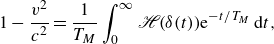
The rectilinear walking speed,
 $v_0$
, increases monotonically with the vibrational forcing, approaching the speed limit,
$v_0$
, increases monotonically with the vibrational forcing, approaching the speed limit,
 $c$
, at the Faraday threshold (see figure 2
$c$
, at the Faraday threshold (see figure 2
 $a$
). As the droplet walks faster, the local wave height,
$a$
). As the droplet walks faster, the local wave height,
 $H$
, and wave energy,
$H$
, and wave energy,
 $E$
, both decrease relative to that of a stationary bouncer, denoted
$E$
, both decrease relative to that of a stationary bouncer, denoted
 $H_B$
and
$H_B$
and
 $E_B$
, respectively (see figure 2
$E_B$
, respectively (see figure 2
 $b,\!c$
). The theoretical prediction for the local wave height,
$b,\!c$
). The theoretical prediction for the local wave height,
 $H/H_B = \gamma _D(v_0)$
(see (3.1)), where
$H/H_B = \gamma _D(v_0)$
(see (3.1)), where
 $\gamma _D(v) = 1-v^2/c^2$
is the speed-dependent diminution factor, holds exactly for all
$\gamma _D(v) = 1-v^2/c^2$
is the speed-dependent diminution factor, holds exactly for all
 $\gamma _W \lt \gamma \lt \gamma _F$
. Despite the theoretical prediction for wave energy,
$\gamma _W \lt \gamma \lt \gamma _F$
. Despite the theoretical prediction for wave energy,
 $E/E_B = \gamma _D(v_0)$
(see (3.1)), being formally valid only in the high-memory limit (for which the error in the approximation is of size
$E/E_B = \gamma _D(v_0)$
(see (3.1)), being formally valid only in the high-memory limit (for which the error in the approximation is of size
 $O((k_F l_d)^{-1})$
), our numerical results demonstrate the efficacy of this prediction both within and beyond the high-memory regime. Indeed, the discrepancy between the theoretical and numerical solutions is visually indistinguishable in figure 2
$O((k_F l_d)^{-1})$
), our numerical results demonstrate the efficacy of this prediction both within and beyond the high-memory regime. Indeed, the discrepancy between the theoretical and numerical solutions is visually indistinguishable in figure 2
 $(b,\!c)$
, with the relative error being less than 1 % for all values of
$(b,\!c)$
, with the relative error being less than 1 % for all values of
 $\gamma$
.
$\gamma$
.

Figure 2. The dependence of energy on the steady rectilinear walking speed,
 $v_0$
, computed using (4.3).
$v_0$
, computed using (4.3).
 $(a)$
The free-walking speed increases with the vibrational forcing for
$(a)$
The free-walking speed increases with the vibrational forcing for
 $\gamma _W \lt \gamma \lt \gamma _F$
, approaching the speed limit,
$\gamma _W \lt \gamma \lt \gamma _F$
, approaching the speed limit,
 $c$
, at the Faraday threshold.
$c$
, at the Faraday threshold.
 $(b, c)$
The magnitude of the local wave height,
$(b, c)$
The magnitude of the local wave height,
 $H$
(red squares), and stroboscopic wave energy,
$H$
(red squares), and stroboscopic wave energy,
 $E$
(green diamonds), relative to that of a bouncer (
$E$
(green diamonds), relative to that of a bouncer (
 $H_B$
and
$H_B$
and
 $E_B$
, respectively) as a function of
$E_B$
, respectively) as a function of
 $(b)$
vibrational acceleration,
$(b)$
vibrational acceleration,
 $\gamma$
, and
$\gamma$
, and
 $(c)$
free-walking speed,
$(c)$
free-walking speed,
 $v_0$
. The numerical results coincide with the theoretical predictions
$v_0$
. The numerical results coincide with the theoretical predictions
 $H/H_B = \gamma _D(v_0)$
and
$H/H_B = \gamma _D(v_0)$
and
 $E/E_B = \gamma _D(v_0)$
for steady droplet motion (see § 3) indicated by the black curve, where
$E/E_B = \gamma _D(v_0)$
for steady droplet motion (see § 3) indicated by the black curve, where
 $\gamma _D(v) = 1-v^2/c^2$
is the speed-dependent diminution factor (see (2.4)). The physical parameter values are the same as in figure 1.
$\gamma _D(v) = 1-v^2/c^2$
is the speed-dependent diminution factor (see (2.4)). The physical parameter values are the same as in figure 1.

Figure 3. The dependence of energy on the steady orbital speed,
 $v$
, computed using (4.3) for
$v$
, computed using (4.3) for
 $\gamma / \gamma _F$
taking values 0.9 (blue), 0.95 (green) and 0.98 (red).
$\gamma / \gamma _F$
taking values 0.9 (blue), 0.95 (green) and 0.98 (red).
 $(a)$
The orbital speed oscillates over half the Faraday wavelength as the orbital radius,
$(a)$
The orbital speed oscillates over half the Faraday wavelength as the orbital radius,
 $r_0$
, is increased, approaching the rectilinear walking speed,
$r_0$
, is increased, approaching the rectilinear walking speed,
 $v_0$
, for large radii. The variations in the orbital speed are most pronounced close to the Faraday threshold.
$v_0$
, for large radii. The variations in the orbital speed are most pronounced close to the Faraday threshold.
 $(b, c)$
The magnitude of the local wave height,
$(b, c)$
The magnitude of the local wave height,
 $H$
(squares), and stroboscopic wave energy,
$H$
(squares), and stroboscopic wave energy,
 $E$
(diamonds), relative to that of a bouncer (
$E$
(diamonds), relative to that of a bouncer (
 $H_B$
and
$H_B$
and
 $E_B$
, respectively) as a function of
$E_B$
, respectively) as a function of
 $(b)$
orbital radius,
$(b)$
orbital radius,
 $r_0$
, and
$r_0$
, and
 $(c)$
orbital speed,
$(c)$
orbital speed,
 $v$
. The numerical results coincide with the theoretical predictions
$v$
. The numerical results coincide with the theoretical predictions
 $H/H_B = \gamma _D(v)$
and
$H/H_B = \gamma _D(v)$
and
 $E/E_B = \gamma _D(v)$
for steady droplet motion (see § 3) indicated by the black curve, where
$E/E_B = \gamma _D(v)$
for steady droplet motion (see § 3) indicated by the black curve, where
 $\gamma _D(v) = 1-v^2/c^2$
is the speed-dependent diminution factor (see (2.4)). The physical parameter values are the same as in figure 1.
$\gamma _D(v) = 1-v^2/c^2$
is the speed-dependent diminution factor (see (2.4)). The physical parameter values are the same as in figure 1.
A similar physical picture emerges for orbital states. As the orbital radius,
 $r_0$
, is increased, the orbital speed,
$r_0$
, is increased, the orbital speed,
 $v$
, varies with orbital radius, oscillating over half the Faraday wavelength, before approaching the rectilinear walking speed,
$v$
, varies with orbital radius, oscillating over half the Faraday wavelength, before approaching the rectilinear walking speed,
 $v_0$
, in the large-radius limit (see figure 3
$v_0$
, in the large-radius limit (see figure 3
 $a$
). This speed modulation is a consequence of the increased influence of the droplet’s wake on its motion at high orbital memory (Oza et al. Reference Oza, Harris, Rosales and Bush2014a
), with similar variations in the local wave height,
$a$
). This speed modulation is a consequence of the increased influence of the droplet’s wake on its motion at high orbital memory (Oza et al. Reference Oza, Harris, Rosales and Bush2014a
), with similar variations in the local wave height,
 $H$
, and wave energy,
$H$
, and wave energy,
 $E$
, evident as the orbital radius is increased (see figure 3
$E$
, evident as the orbital radius is increased (see figure 3
 $b$
). Despite this more complex dependence on orbital speed, the theoretical predictions prescribed by the speed-dependent diminution factor,
$b$
). Despite this more complex dependence on orbital speed, the theoretical predictions prescribed by the speed-dependent diminution factor,
 $\gamma _D$
, are in excellent agreement with the numerical results across a wide range of memory and orbital radius. Indeed, the dependences of normalised local wave height,
$\gamma _D$
, are in excellent agreement with the numerical results across a wide range of memory and orbital radius. Indeed, the dependences of normalised local wave height,
 $H/H_B$
, and wave energy,
$H/H_B$
, and wave energy,
 $E/E_B$
, on orbital speed collapse onto the curve
$E/E_B$
, on orbital speed collapse onto the curve
 $\gamma _D(v)$
for all values of
$\gamma _D(v)$
for all values of
 $\gamma$
(see figure 3
$\gamma$
(see figure 3
 $c$
), underscoring the universal dependence of energy on speed in orbital pilot-wave dynamics.
$c$
), underscoring the universal dependence of energy on speed in orbital pilot-wave dynamics.
Of particular interest is the partitioning of energy in pilot-wave hydrodynamics, which we quantify here for steady walking and orbiting states. To do so, we define the total stroboscopic energy as
 \begin{equation} \mathcal {E} = \frac {1}{2}m|\dot{\boldsymbol{x}}_{{\kern-1.5pt}p}|^2 + mgH + E, \end{equation}
representing the sum of kinetic, gravitational potential and wave energies. For steady walking and orbiting, we apply the approximations given by (3.1) (as verified in figures 2 and 3) to deduce from (4.4) the approximate relationship
 \begin{equation} \mathcal {E} = \frac {1}{2}m|\dot{\boldsymbol{x}}_{{\kern-1.5pt}p}|^2 + \gamma _D(|\dot{\boldsymbol{x}}_{{\kern-1.5pt}p}|)\big (mg H_B + E_B\big), \end{equation}
which makes clear the dependence on the speed-dependent diminution factor,
 $\gamma _D$
, and the relative sizes of the local wave height,
$\gamma _D$
, and the relative sizes of the local wave height,
 $H_B$
, and wave energy,
$H_B$
, and wave energy,
 $E_B$
, for stationary bouncing. In particular, we see from (4.5) that the contribution of kinetic energy to the total stroboscopic energy,
$E_B$
, for stationary bouncing. In particular, we see from (4.5) that the contribution of kinetic energy to the total stroboscopic energy,
 $\mathcal {E}$
, increases with droplet speed, while the contributions of wave and gravitational potential energies both decrease.
$\mathcal {E}$
, increases with droplet speed, while the contributions of wave and gravitational potential energies both decrease.

Figure 4. The dependence of the energy partitioning on vibrational forcing for stationary bouncing (dashed curves) and steady walking at the free-walking speed,
 $v_0$
(solid curves).
$v_0$
(solid curves).
 $(a)$
The contribution to the total energy,
$(a)$
The contribution to the total energy,
 $\mathcal {E}$
(grey, see (4.4)), in terms of the stroboscopic wave energy,
$\mathcal {E}$
(grey, see (4.4)), in terms of the stroboscopic wave energy,
 $E$
(red), droplet gravitational potential energy,
$E$
(red), droplet gravitational potential energy,
 $mg H$
(blue), and droplet kinetic energy,
$mg H$
(blue), and droplet kinetic energy,
 $\frac {1}{2}m v_0^2$
(black). The total energy is normalised by that of a bouncer at the walking threshold,
$\frac {1}{2}m v_0^2$
(black). The total energy is normalised by that of a bouncer at the walking threshold,
 $\mathcal {E}(\gamma _W)$
. The wave energy diverges in the high-memory limit for both bouncing and walking. Notably, the droplet gravitational potential energy diverges at high memory for a bouncer, yet decreases towards a finite value (comparable to the kinetic energy) for a walker.
$\mathcal {E}(\gamma _W)$
. The wave energy diverges in the high-memory limit for both bouncing and walking. Notably, the droplet gravitational potential energy diverges at high memory for a bouncer, yet decreases towards a finite value (comparable to the kinetic energy) for a walker.
 $(b)$
The relative contributions of each type of energy to the total energy, with the wave energy dominating in the high-memory limit. The physical parameter values are the same as in figure 1.
$(b)$
The relative contributions of each type of energy to the total energy, with the wave energy dominating in the high-memory limit. The physical parameter values are the same as in figure 1.

Figure 5. The dependence of the energy partitioning on the orbital radius for steady orbiting at
 $\gamma /\gamma _F = 0.95$
.
$\gamma /\gamma _F = 0.95$
.
 $(a)$
The contributions to the total energy,
$(a)$
The contributions to the total energy,
 $\mathcal {E}$
(grey, see (4.4)), from the stroboscopic wave energy,
$\mathcal {E}$
(grey, see (4.4)), from the stroboscopic wave energy,
 $E$
(red), droplet gravitational potential energy,
$E$
(red), droplet gravitational potential energy,
 $mg H$
(blue), and droplet kinetic energy,
$mg H$
(blue), and droplet kinetic energy,
 $\frac {1}{2}m v^2$
(black). The total energy is normalised by that of a bouncer at the walking threshold,
$\frac {1}{2}m v^2$
(black). The total energy is normalised by that of a bouncer at the walking threshold,
 $\mathcal {E}(\gamma _W)$
.
$\mathcal {E}(\gamma _W)$
.
 $(b)$
Energy partition of
$(b)$
Energy partition of
 $\mathcal {E}$
, with minima in the wave and gravitational potential energies corresponding to maxima in the kinetic energy. The physical parameter values are the same as in figure 1.
$\mathcal {E}$
, with minima in the wave and gravitational potential energies corresponding to maxima in the kinetic energy. The physical parameter values are the same as in figure 1.
In figure 4, we present the dependence of the total stroboscopic energy on the vibrational forcing for stationary bouncing and steady walking. For both bouncing and walking, the wave energy diverges in the high-memory limit, where the wave field spans the entire plane and so is the main contributor to the total energy (see Appendix C). For steady walking, the kinetic energy increases with the vibrational forcing (consistent with the walking speed curve in figure 2
 $a$
), while the gravitational potential energy decreases, approaching a finite value in the high-memory limit. The adjustment of the droplet from its wave crest to a region with higher slope is also evident in the wave-field plots in figure 1. Finally, we note that although the gravitational potential energy of a bouncer diverges as the Faraday threshold is approached, this contribution is subdominant to the wave energy, with
$a$
), while the gravitational potential energy decreases, approaching a finite value in the high-memory limit. The adjustment of the droplet from its wave crest to a region with higher slope is also evident in the wave-field plots in figure 1. Finally, we note that although the gravitational potential energy of a bouncer diverges as the Faraday threshold is approached, this contribution is subdominant to the wave energy, with
 $mgH_B \ll E_B$
at high memory (see (4.5)).
$mgH_B \ll E_B$
at high memory (see (4.5)).
Similar trends for orbital motion are evident in figure 5. At high memory, the wave energy dominates the droplet kinetic and gravitational potential energies. We note that modulations in the droplet speed with the orbital radius lead to peaks in the partitioning of kinetic energy, and corresponding troughs in the partitioning of wave energy. While it is not easily discernible from figure 5
 $(b)$
, the droplet gravitational potential energy oscillates in a manner similar to that of the wave energy, by virtue of the relationships
$(b)$
, the droplet gravitational potential energy oscillates in a manner similar to that of the wave energy, by virtue of the relationships
 $H/H_B = E/E_B = \gamma _D(v)$
. As the vibrational forcing is progressively increased, the peaks and troughs in figure 5
$H/H_B = E/E_B = \gamma _D(v)$
. As the vibrational forcing is progressively increased, the peaks and troughs in figure 5
 $(b)$
become more pronounced, and the wave energy dominates the total energy.
$(b)$
become more pronounced, and the wave energy dominates the total energy.
4.2. Onset of unstable orbital motion
To investigate the efficacy of (3.2) for slowly varying and periodic states, we consider the onset of orbital instability in a rotating frame. A droplet walking in a rotating frame moves in response to a Coriolis force,
 $\boldsymbol{F} = -2m \boldsymbol{\Omega } \times \dot{\boldsymbol{x}}_{{\kern-1.5pt}p}$
, where the rotation vector,
$\boldsymbol{F} = -2m \boldsymbol{\Omega } \times \dot{\boldsymbol{x}}_{{\kern-1.5pt}p}$
, where the rotation vector,
 $\boldsymbol{\Omega } = \Omega \boldsymbol{e}_z$
, is orientated vertically, perpendicular to the droplet’s plane of motion (Fort et al. Reference Fort, Eddi, Boudaoud, Moukhtar and Couder2010; Harris & Bush Reference Harris and Bush2014; Oza et al. Reference Oza, Harris, Rosales and Bush2014a
). For a droplet moving at steady speed
$\boldsymbol{\Omega } = \Omega \boldsymbol{e}_z$
, is orientated vertically, perpendicular to the droplet’s plane of motion (Fort et al. Reference Fort, Eddi, Boudaoud, Moukhtar and Couder2010; Harris & Bush Reference Harris and Bush2014; Oza et al. Reference Oza, Harris, Rosales and Bush2014a
). For a droplet moving at steady speed
 $v = r_0 \omega$
along a circular orbit of radius
$v = r_0 \omega$
along a circular orbit of radius
 $r_0$
, we deduce from pilot-wave system (2.1) the radial and tangential force balances:
$r_0$
, we deduce from pilot-wave system (2.1) the radial and tangential force balances:
 \begin{align} -m r_0 \omega ^2 = -\frac {mgA}{T_F} \int _0^\infty \mathscr {H}\, \, '\left (2 r_0 \sin \left (\frac {\omega t}{2}\right)\right)\sin \left (\frac {\omega t}{2}\right)\mathrm {e}^{-t/T_M}\, \mathrm {d}t + 2m\varOmega r_0 \omega, \end{align}
 \begin{align} D r_0 \omega = -\frac {mgA}{T_F}\int _0^\infty \mathscr {H}\, \, '\left (2 r_0 \sin \left (\frac {\omega t}{2}\right)\right)\cos \left (\frac {\omega t}{2}\right)\mathrm {e}^{-t/T_M}\, \mathrm {d}t,\qquad \end{align}
where
 $\mathscr {H}\, \, '(r)$
denotes the derivative of
$\mathscr {H}\, \, '(r)$
denotes the derivative of
 $\mathscr {H}\,\,$
with respect to
$\mathscr {H}\,\,$
with respect to
 $r$
(with an odd extension so as to be defined over the real line). Notably, one may apply integration by parts to the tangential force balance (4.6b
) to deduce the equation for local wave height (4.3) (Oza et al. Reference Oza, Harris, Rosales and Bush2014a
; Liu et al. Reference Liu, Durey and Bush2023). Following Oza et al. (Reference Oza, Harris, Rosales and Bush2014a
), we parameterise the circular orbits by their orbital radius for a fixed vibrational forcing: specifically, we fix
$r$
(with an odd extension so as to be defined over the real line). Notably, one may apply integration by parts to the tangential force balance (4.6b
) to deduce the equation for local wave height (4.3) (Oza et al. Reference Oza, Harris, Rosales and Bush2014a
; Liu et al. Reference Liu, Durey and Bush2023). Following Oza et al. (Reference Oza, Harris, Rosales and Bush2014a
), we parameterise the circular orbits by their orbital radius for a fixed vibrational forcing: specifically, we fix
 $r_0$
and use (4.6b
) (or (4.3)) to solve for the orbital frequency,
$r_0$
and use (4.6b
) (or (4.3)) to solve for the orbital frequency,
 $\omega$
, and then use (4.6a
) to determine the corresponding bath rotation rate.
$\omega$
, and then use (4.6a
) to determine the corresponding bath rotation rate.
We investigate the evolution of the local wave height,
 $H(t)$
, and stroboscopic wave energy,
$H(t)$
, and stroboscopic wave energy,
 $E(t)$
, for an oscillatory instability whose corresponding perturbation grows towards a 2-wobble (Harris & Bush Reference Harris and Bush2014; Oza et al. Reference Oza, Wind-Willassen, Harris, Rosales and Bush2014b
). We thus anticipate that (3.2) (with
$E(t)$
, for an oscillatory instability whose corresponding perturbation grows towards a 2-wobble (Harris & Bush Reference Harris and Bush2014; Oza et al. Reference Oza, Wind-Willassen, Harris, Rosales and Bush2014b
). We thus anticipate that (3.2) (with
 $V = 0$
) will hold sufficiently close to the instability threshold, for which the instability time scale greatly exceeds the orbital time scale. This behaviour is evidenced in figure 6, for which the local wave height and wave energy when averaged over one speed cycle (denoted
$V = 0$
) will hold sufficiently close to the instability threshold, for which the instability time scale greatly exceeds the orbital time scale. This behaviour is evidenced in figure 6, for which the local wave height and wave energy when averaged over one speed cycle (denoted
 $\langle H \rangle /H_B$
and
$\langle H \rangle /H_B$
and
 $\langle E \rangle /E_B$
, respectively) agree closely with the theoretical predictions made by (3.2) during both the unstable transient and the periodic 2-wobble. Notably, the theoretical prediction for
$\langle E \rangle /E_B$
, respectively) agree closely with the theoretical predictions made by (3.2) during both the unstable transient and the periodic 2-wobble. Notably, the theoretical prediction for
 $\langle E \rangle / E_B$
slightly exceeds the accompanying numerical result; this discrepancy is a direct consequence of the high-memory approximation made when deriving (2.17), and so will be less significant closer to the Faraday threshold.
$\langle E \rangle / E_B$
slightly exceeds the accompanying numerical result; this discrepancy is a direct consequence of the high-memory approximation made when deriving (2.17), and so will be less significant closer to the Faraday threshold.
We further test the efficacy of our theoretical predictions by comparing in figure 7 the evolution of
 $\mathrm {d}E/\mathrm {d}t$
in the simulations with the theoretical prediction prescribed by (2.17). This investigation is based on the same simulation as in figure 6, but with the focus shifted onto the instantaneous wave energy, rather than that time-averaged over each speed cycle. For the numerical simulations,
$\mathrm {d}E/\mathrm {d}t$
in the simulations with the theoretical prediction prescribed by (2.17). This investigation is based on the same simulation as in figure 6, but with the focus shifted onto the instantaneous wave energy, rather than that time-averaged over each speed cycle. For the numerical simulations,
 $\mathrm {d}E/\mathrm {d}t$
is computed using a second-order finite-difference approximation of
$\mathrm {d}E/\mathrm {d}t$
is computed using a second-order finite-difference approximation of
 $E(t)$
, as defined by (2.7). For the theoretical prediction, the numerically computed values of
$E(t)$
, as defined by (2.7). For the theoretical prediction, the numerically computed values of
 $E(t)$
and
$E(t)$
and
 $H(t)$
are substituted into the right-hand side of (2.17). Akin to figure 6
$H(t)$
are substituted into the right-hand side of (2.17). Akin to figure 6
 $(d)$
, the theoretical prediction for
$(d)$
, the theoretical prediction for
 $\mathrm {d}E/\mathrm {d}t$
is typically slightly larger than its numerical counterpart, as is most apparent in the unstable transient (see figure 7
$\mathrm {d}E/\mathrm {d}t$
is typically slightly larger than its numerical counterpart, as is most apparent in the unstable transient (see figure 7
 $a$
). Nevertheless, there is excellent agreement when the droplet executes the periodic 2-wobble, as demonstrated in figure 7
$a$
). Nevertheless, there is excellent agreement when the droplet executes the periodic 2-wobble, as demonstrated in figure 7
 $(b)$
for the final two orbital periods. Our findings verify that (2.17) may be reliably used to investigate the evolution of energy in pilot-wave hydrodynamics, forming a platform on which to base future investigations of unsteady systems.
$(b)$
for the final two orbital periods. Our findings verify that (2.17) may be reliably used to investigate the evolution of energy in pilot-wave hydrodynamics, forming a platform on which to base future investigations of unsteady systems.

Figure 6. Wobbling motion of an inertial orbit in a frame rotating at
 $\varOmega = -2.78 \mbox { rad s}^{-1}$
and vibrating with
$\varOmega = -2.78 \mbox { rad s}^{-1}$
and vibrating with
 $\gamma /\gamma _F = 0.96$
.
$\gamma /\gamma _F = 0.96$
.
 $(a)$
Droplet trajectory following a small perturbation from an anticlockwise circular orbit of radius
$(a)$
Droplet trajectory following a small perturbation from an anticlockwise circular orbit of radius
 $r_0/\lambda _F = 0.8$
. After an initial transient, the trajectory approaches a 2-wobble (grey curve, with the final orbital period denoted in blue).
$r_0/\lambda _F = 0.8$
. After an initial transient, the trajectory approaches a 2-wobble (grey curve, with the final orbital period denoted in blue).
 $(b)$
Evolution of the droplet speed (black curve). The red diamonds denote the maxima of each speed cycle, over which the average speed,
$(b)$
Evolution of the droplet speed (black curve). The red diamonds denote the maxima of each speed cycle, over which the average speed,
 $\bar v = \langle |\dot{\boldsymbol{x}}_{{\kern-1.5pt}p}|^2 \rangle ^{1/2}$
, is computed (see § 3).
$\bar v = \langle |\dot{\boldsymbol{x}}_{{\kern-1.5pt}p}|^2 \rangle ^{1/2}$
, is computed (see § 3).
 $(c,d)$
The black curves denote the evolution of
$(c,d)$
The black curves denote the evolution of
 $(c)$
the local wave height,
$(c)$
the local wave height,
 $H/H_B$
, and
$H/H_B$
, and
 $(d)$
the wave energy,
$(d)$
the wave energy,
 $E/E_B$
, each normalised by that of a stationary bouncer at the same memory. Time is scaled by the orbital period,
$E/E_B$
, each normalised by that of a stationary bouncer at the same memory. Time is scaled by the orbital period,
 $T_O = 2\pi /\omega$
, of the initial circular orbit. The red circles denote the average values of
$T_O = 2\pi /\omega$
, of the initial circular orbit. The red circles denote the average values of
 $H/H_B$
and
$H/H_B$
and
 $E/E_B$
over each speed cycle, and the blue curve denotes the corresponding theoretical prediction given by
$E/E_B$
over each speed cycle, and the blue curve denotes the corresponding theoretical prediction given by
 $\langle H \rangle /H_B = \langle E \rangle /E_B = \gamma _D(\bar {v})$
(see (3.2)). The physical parameter values are the same as in figure 1.
$\langle H \rangle /H_B = \langle E \rangle /E_B = \gamma _D(\bar {v})$
(see (3.2)). The physical parameter values are the same as in figure 1.

Figure 7. The rate of change of wave energy for a droplet executing the same wobbling trajectory as in figure 6.
 $(a)$
The black curve denotes
$(a)$
The black curve denotes
 $\mathrm {d}E/\mathrm {d}t$
computed from the simulation, and the blue curve denotes
$\mathrm {d}E/\mathrm {d}t$
computed from the simulation, and the blue curve denotes
 $\mathrm {d}E/\mathrm {d}t$
as computed from the theoretical prediction (2.17). Time is scaled by the orbital period,
$\mathrm {d}E/\mathrm {d}t$
as computed from the theoretical prediction (2.17). Time is scaled by the orbital period,
 $T_O$
, of the initial unstable orbit, and wave energy is normalised by that of a stationary bouncer,
$T_O$
, of the initial unstable orbit, and wave energy is normalised by that of a stationary bouncer,
 $E_B$
, at the same memory.
$E_B$
, at the same memory.
 $(b)$
Zoom-in of
$(b)$
Zoom-in of
 $(a)$
underscores the efficacy of the theoretical prediction when the droplet executes a 2-wobble.
$(a)$
underscores the efficacy of the theoretical prediction when the droplet executes a 2-wobble.
5. Discussion
Our study has yielded several new insights into the energetics of pilot-wave hydrodynamics. The walking droplet system is damped and driven, with energy input from the bath vibration and energy dissipated through the action of viscosity. We have paid particular attention to the cases in which these energy inputs and outputs balance, specifically steady and periodic dynamical states, slowly varying states and statistically steady states. For such states, our study illustrates how the partitioning of energy between droplet kinetic energy, droplet gravitational energy and wave energy depends on the system memory. It further illustrates how this partitioning evolves with time for unsteady states. Specifically, the rate of change of droplet energy (2.5) is prescribed by the local wave amplitude relative to that of a bouncer and the diminution factor,
 $\gamma _D(|\dot{\boldsymbol{x}}_{{\kern-1.5pt}p}|)$
, which decreases with the droplet’s speed. The rate of change of wave energy (2.17) also depends on the instantaneous wave energy relative to that of a bouncer, and thus the diminution factor,
$\gamma _D(|\dot{\boldsymbol{x}}_{{\kern-1.5pt}p}|)$
, which decreases with the droplet’s speed. The rate of change of wave energy (2.17) also depends on the instantaneous wave energy relative to that of a bouncer, and thus the diminution factor,
 $\gamma _D$
. Notably, the walker’s wave-induced added mass,
$\gamma _D$
. Notably, the walker’s wave-induced added mass,
 $m\gamma _B(|\dot{\boldsymbol{x}}_{{\kern-1.5pt}p}|)$
, also decreases with its speed (Bush et al. Reference Bush, Oza and Moláček2014). A comparison between
$m\gamma _B(|\dot{\boldsymbol{x}}_{{\kern-1.5pt}p}|)$
, also decreases with its speed (Bush et al. Reference Bush, Oza and Moláček2014). A comparison between
 $\gamma _B$
and the energy diminution factor,
$\gamma _B$
and the energy diminution factor,
 $\gamma _D$
, is presented in Appendix D.
$\gamma _D$
, is presented in Appendix D.
Our theoretical developments may be extended in a straightforward fashion in order to treat the energetics of
 $N$
interacting droplets with constant impact phase, as outlined in Appendix E. In particular, insight into multiple-droplet systems (e.g. lattices or rings) may be gained through consideration of the wave energy,
$N$
interacting droplets with constant impact phase, as outlined in Appendix E. In particular, insight into multiple-droplet systems (e.g. lattices or rings) may be gained through consideration of the wave energy,
 $E(t)$
, which evolves according to (E7). For quasi-steady droplet motion, the correspondence
$E(t)$
, which evolves according to (E7). For quasi-steady droplet motion, the correspondence
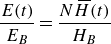 \begin{equation} \frac {E(t)}{E_B} = \frac {N\,\overline{\!H}(t)}{H_B} \end{equation}
holds, where
 $\,\overline{\!H}$
is the average height of the wave field beneath the droplets, which incorporates wave-mediated inter-droplet spatio-temporal correlations (see (E8)). Consequently, the evolution of the mean lattice wave height may be used as a proxy for that of wave energy for slowly evolving lattices. The decrease in average droplet height between discrete rearrangements of unstable ring structures noted by Couchman & Bush (Reference Couchman and Bush2020) was thus accompanied by a decrease in the energy of the global pilot-wave field, and so reflects the tendency of multiple-droplet systems to minimise their total energy. We note, however, that (5.1) does not account for dynamic or spatial variations in the droplets’ impact phase, and so is not necessarily applicable to irregular or unsteady lattice structures.
$\,\overline{\!H}$
is the average height of the wave field beneath the droplets, which incorporates wave-mediated inter-droplet spatio-temporal correlations (see (E8)). Consequently, the evolution of the mean lattice wave height may be used as a proxy for that of wave energy for slowly evolving lattices. The decrease in average droplet height between discrete rearrangements of unstable ring structures noted by Couchman & Bush (Reference Couchman and Bush2020) was thus accompanied by a decrease in the energy of the global pilot-wave field, and so reflects the tendency of multiple-droplet systems to minimise their total energy. We note, however, that (5.1) does not account for dynamic or spatial variations in the droplets’ impact phase, and so is not necessarily applicable to irregular or unsteady lattice structures.
It is worth emphasising the generality of our results, but also noting their limitations. In our theoretical developments, we have assumed only that the axisymmetric wave kernel oscillates over the Faraday wavelength and decays exponentially at infinity, with the spatial decay length increasing with proximity to the Faraday threshold. Our results thus apply not only to the particular wave kernel considered in our numerical examples (§ 4) but to any such pilot-wave form. As a caveat, we note that our results have been deduced from the stroboscopic model, which is based on the assumption of resonance between the droplet and its guiding wave. The role of impact phase is somewhat obscured in the stroboscopic formulation, but becomes clear when one recalls that all of our energetic formulations have been made in terms of the stroboscopic wave height,
 $h({\boldsymbol{x}},t)$
, rather than the temporally oscillating wave field,
$h({\boldsymbol{x}},t)$
, rather than the temporally oscillating wave field,
 $\eta ({\boldsymbol{x}},t) = h({\boldsymbol{x}},t) \cos (\pi ft)/\mathscr {C}$
. Notably, the energy of the stroboscopic wave field,
$\eta ({\boldsymbol{x}},t) = h({\boldsymbol{x}},t) \cos (\pi ft)/\mathscr {C}$
. Notably, the energy of the stroboscopic wave field,
 $E$
, is related to the energy of the temporally oscillating wave field averaged over one Faraday period,
$E$
, is related to the energy of the temporally oscillating wave field averaged over one Faraday period,
 $\overline {\mathscr {E}}$
, via
$\overline {\mathscr {E}}$
, via
 $\overline {\mathscr {E}} = ({1}/{2})E/\mathscr {C}\ ^2$
, so the two energies are proportional. As the memory is increased, the phase of drop impact relative to the wave oscillation,
$\overline {\mathscr {E}} = ({1}/{2})E/\mathscr {C}\ ^2$
, so the two energies are proportional. As the memory is increased, the phase of drop impact relative to the wave oscillation,
 $\mathscr {C}$
, also changes, and with it the relative magnitudes of the wave and droplet energies. This dependence is not captured with the stroboscopic model, which assumes that the impact phase is independent of memory. Nevertheless, our results may be applied given the value of
$\mathscr {C}$
, also changes, and with it the relative magnitudes of the wave and droplet energies. This dependence is not captured with the stroboscopic model, which assumes that the impact phase is independent of memory. Nevertheless, our results may be applied given the value of
 $\mathscr {C}$
at a particular memory, as may be measured experimentally.
$\mathscr {C}$
at a particular memory, as may be measured experimentally.
While the stroboscopic model has been successful in rationalising a number of phenomena in pilot-wave hydrodynamics, it is known to have shortcomings in situations where the droplet’s impact phase varies owing to its interaction with a time-varying wave field, as may arise at high memory (Wind-Willassen et al. Reference Wind-Willassen, Moláček, Harris and Bush2013) and in closed settings (Harris et al. Reference Harris, Moukhtar, Fort, Couder and Bush2013; Durey et al. Reference Durey, Milewski and Wang2020; Abraham et al. Reference Abraham, Malkov, Ljubetic, Durey and Sáenz2024). Relaxation of the stroboscopic approximation requires consideration of the droplet’s vertical dynamics (Moláček & Bush Reference Moláček and Bush2013a ; Couchman et al. Reference Couchman, Turton and Bush2019; Primkulov et al. Reference Primkulov, Evans, Been and Bush2025). Consideration of the energetics in this more general setting will yield insight into the myriad complex periodic, aperiodic and chaotic walking states arising at high memory (Moláček & Bush Reference Moláček and Bush2013b ; Wind-Willassen et al. Reference Wind-Willassen, Moláček, Harris and Bush2013) and will be the subject of future work.
Acknowledgements.
The authors thank N. Liu for valuable discussions and D. M. Harris for the photo used in our graphical abstract.
Funding.
J.W.M.B. gratefully acknowledges the generous financial support of the NSF through grant CMMI-2154151, and the Office of Naval Research through grant N000014-24-1-2232.
Declaration of interests.
The authors report no conflict of interest.
Data availability statement.
Data sharing not applicable – no new data generated.
Appendix A. Energy budget
In contrast to the majority of studies on the spontaneous formation of waves above the Faraday threshold (Kumar & Tuckerman Reference Kumar and Tuckerman1994; Kumar Reference Kumar1996), the Faraday waves in the walking-droplet system are subcritical, yet sustained by repeated impacts of the droplet on the bath. The energy budget is complex: the energy injection depends on the interference of the waves generated by the moving droplet, and the bath vibration serves to increase the longevity of the waves generated at each impact. These two sources of energy injection may be distinguished by recasting the droplet (2.5) and wave (2.17) energy evolution equations as
 \begin{align} \frac {\mathrm {d} {E_p}}{\mathrm {d} {t}} + D|\dot{\boldsymbol{x}}_{{\kern-1.5pt}p}|^2 + \frac {mgH(t)}{T_d} = \frac {mgA}{T_F} + \left (\frac {1}{T_d} - \frac {1}{T_M}\right)mgH(t), \end{align}
 \begin{align} \frac {1}{2}\frac {\mathrm {d}E}{\mathrm {d}t} + \frac {E(t)}{T_d} = \frac {E_B H(t)}{T_M H_B} + \left (\frac {1}{T_d} - \frac {1}{T_M}\right)E(t).\qquad\quad \end{align}
In both energy equations, the terms on the right-hand side correspond to energy injection through wave creation and bath vibration, respectively. The left-hand side thus describes the energy dissipation, as governed by work done on the droplet by drag (in (A1a
) only) and dissipation of the wave field over
 $T_d$
, the viscous decay time in the absence of vibration.
$T_d$
, the viscous decay time in the absence of vibration.
We proceed to more closely examine the energy injection in (A1). We first note that the energy injection from the bath vibration may be characterised in terms of the effective growth rate
 \begin{equation} \frac {1}{T_d} - \frac {1}{T_M} = \frac {\gamma /\gamma _F}{T_d}, \end{equation}
which describes the decrease in the wave decay rate resulting from bath vibration (Benjamin & Ursell Reference Benjamin and Ursell1954). The energy injection via wave creation is more subtle. The droplet energy injection rate,
 $mgA/T_F$
in (A1a
), is constant, a consequence of the waves generated along the droplet’s path being of equal amplitude. In contrast, the wave energy injection rate,
$mgA/T_F$
in (A1a
), is constant, a consequence of the waves generated along the droplet’s path being of equal amplitude. In contrast, the wave energy injection rate,
 $E_B H(t)/T_M H_B$
in (A1b
), depends on the local wave height,
$E_B H(t)/T_M H_B$
in (A1b
), depends on the local wave height,
 $H(t)$
, which can vary substantially as the droplet navigates its pilot wave. As the droplet’s dynamics and the constants
$H(t)$
, which can vary substantially as the droplet navigates its pilot wave. As the droplet’s dynamics and the constants
 $A$
,
$A$
,
 $T_M$
,
$T_M$
,
 $H_B$
and
$H_B$
and
 $E_B$
appearing in (A1) depend on the proximity of the vibrational acceleration,
$E_B$
appearing in (A1) depend on the proximity of the vibrational acceleration,
 $\gamma$
, to the Faraday threshold,
$\gamma$
, to the Faraday threshold,
 $\gamma _F$
, we conclude that
$\gamma _F$
, we conclude that
 $\gamma /\gamma _F$
is the primary factor controlling both forms of energy injection. A more detailed investigation of the system’s energy budget will be the subject of future work.
$\gamma /\gamma _F$
is the primary factor controlling both forms of energy injection. A more detailed investigation of the system’s energy budget will be the subject of future work.
Appendix B. Energy evolution for the
 $\mathrm {J}_0(k_F r)$
wave kernel
$\mathrm {J}_0(k_F r)$
wave kernel

For the dynamics of a single droplet, the exponential spatial decay of the wave field is relatively unimportant (Bush Reference Bush2015; Bush & Oza Reference Bush and Oza2021), with investigators thus considering the algebraically tractable wave kernel
 $\mathscr {H}\ (r) = \mathrm {J}_0(k_F r)$
(Oza et al. Reference Oza, Rosales and Bush2013). In this case, the notion of wave energy is somewhat nebulous, with the defining integrals (2.7) of the wave field over the plane being divergent. To circumnavigate this issue, Labousse et al. (Reference Labousse, Perrard, Couder and Fort2016b
) and Hubert et al. (Reference Hubert, Perrard, Vandewalle and Labousse2022) defined a corresponding wave intensity, denoted
$\mathscr {H}\ (r) = \mathrm {J}_0(k_F r)$
(Oza et al. Reference Oza, Rosales and Bush2013). In this case, the notion of wave energy is somewhat nebulous, with the defining integrals (2.7) of the wave field over the plane being divergent. To circumnavigate this issue, Labousse et al. (Reference Labousse, Perrard, Couder and Fort2016b
) and Hubert et al. (Reference Hubert, Perrard, Vandewalle and Labousse2022) defined a corresponding wave intensity, denoted
 $I(t)$
, that retained the key features of wave energy whilst being non-divergent. When accounting for the influence of gravitational potential and surface energies for a linear stroboscopic wave field, the wave intensity is defined as (Liu et al. Reference Liu, Durey and Bush2023)
$I(t)$
, that retained the key features of wave energy whilst being non-divergent. When accounting for the influence of gravitational potential and surface energies for a linear stroboscopic wave field, the wave intensity is defined as (Liu et al. Reference Liu, Durey and Bush2023)
 \begin{equation} I(t) = \lim _{R_0\rightarrow \infty } \frac {1}{2R_0} \left [\iint _{|{\boldsymbol{x}}|\lt R_0} \Big (\rho g h^2({\boldsymbol{x}},t) + \sigma |\nabla h|^2\Big)\,\mathrm {d}{\boldsymbol{x}}\right], \end{equation}
with
 $h({\boldsymbol{x}},t)$
defined by (2.1b
) for
$h({\boldsymbol{x}},t)$
defined by (2.1b
) for
 $\mathscr {H}\ (r) = \mathrm {J}_0(k_F r)$
. Notably, the wave intensity defined in (B1) has units of energy per unit length. Owing to the monochromatic form of the pilot wave, one may equivalently express the wave intensity as (Liu et al. Reference Liu, Durey and Bush2023)
$\mathscr {H}\ (r) = \mathrm {J}_0(k_F r)$
. Notably, the wave intensity defined in (B1) has units of energy per unit length. Owing to the monochromatic form of the pilot wave, one may equivalently express the wave intensity as (Liu et al. Reference Liu, Durey and Bush2023)
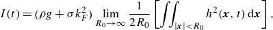 \begin{equation} I(t) = \Big (\rho g + \sigma k_F^2\Big) \lim _{R_0\rightarrow \infty } \frac {1}{2R_0} \left [\iint _{|{\boldsymbol{x}}|\lt R_0} h^2({\boldsymbol{x}},t)\,\mathrm {d}{\boldsymbol{x}}\right], \end{equation}
which forms the basis for our analysis.
Wave intensity defined in this limiting sense may be better understood by projecting the monochromatic wave field onto the orthogonal eigenfunctions
 $\varPhi _n({\boldsymbol{x}}, k_F) = \mathrm {J}_n(k_F r) \mathrm {e}^{\mathrm {i} n \theta }$
, in a manner similar to § 2.3. Specifically, by expressing
$\varPhi _n({\boldsymbol{x}}, k_F) = \mathrm {J}_n(k_F r) \mathrm {e}^{\mathrm {i} n \theta }$
, in a manner similar to § 2.3. Specifically, by expressing
 \begin{equation} h({\boldsymbol{x}},t) = \sum _{n=-\infty }^\infty a_n(t) \varPhi _n({\boldsymbol{x}},k_F), \mbox { where } a_n(t) = \frac {H_B}{T_M} \int _{-\infty }^t \varPhi _n^*({\boldsymbol{x}}_{{\kern-1.5pt}p}(s), k_F) \mathrm {e}^{-(t-s)/T_M} {\, \mathrm {d}s} \end{equation}
and
 $H_B = AT_M/T_F$
is the amplitude of the bouncer wave field, it follows from an application of Parseval’s theorem that (Labousse et al. Reference Labousse, Perrard, Couder and Fort2016b
; Hubert et al. Reference Hubert, Perrard, Vandewalle and Labousse2022; Liu et al. Reference Liu, Durey and Bush2023)
$H_B = AT_M/T_F$
is the amplitude of the bouncer wave field, it follows from an application of Parseval’s theorem that (Labousse et al. Reference Labousse, Perrard, Couder and Fort2016b
; Hubert et al. Reference Hubert, Perrard, Vandewalle and Labousse2022; Liu et al. Reference Liu, Durey and Bush2023)
 \begin{equation} I(t) = I_B\sum _{n=-\infty }^{\infty } \frac {|a_n(t)|^2}{H_B^2}, \end{equation}
where
 \begin{equation} I_B = \Big (\rho g + \sigma k_F^2\Big) \lim _{R_0\rightarrow \infty } \frac {1}{2R_0} \left [\iint _{|{\boldsymbol{x}}|\lt R_0} \big [H_B \mathrm {J}_0(k_F|{\boldsymbol{x}}|)\big]^2\,\mathrm {d}{\boldsymbol{x}}\right] = \Big (\rho g + \sigma k_F^2\Big) \frac {H_B^2}{k_F} \end{equation}
is the wave intensity of a bouncer.
Notably, (B4) has the same algebraic form as (2.13c
), but without the
 $O ((k_F^2 l_d)^{-1})$
correction valid in the high-memory limit; indeed, no approximations have been made when deriving (B4) from (B1). We may thus exploit this correspondence to perform a series of algebraic steps identical to those presented in § 2.3 to derive, without approximation, the evolution of wave intensity:
$O ((k_F^2 l_d)^{-1})$
correction valid in the high-memory limit; indeed, no approximations have been made when deriving (B4) from (B1). We may thus exploit this correspondence to perform a series of algebraic steps identical to those presented in § 2.3 to derive, without approximation, the evolution of wave intensity:
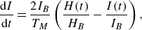 \begin{equation} \frac {\mathrm {d} {I}}{\mathrm {d} {t}} = \frac {2I_B}{T_M}\left (\frac {H(t)}{H_B} - \frac {I(t)}{I_B}\right), \end{equation}
where
 $H(t) = h({\boldsymbol{x}}_{{\kern-1.5pt}p},t)$
is the local wave height. Notably, (B6) is the analogue of the wave energy evolution equation (2.17), thereby demonstrating the generality of the evolution of energy-like wave quantities in terms of the local wave height,
$H(t) = h({\boldsymbol{x}}_{{\kern-1.5pt}p},t)$
is the local wave height. Notably, (B6) is the analogue of the wave energy evolution equation (2.17), thereby demonstrating the generality of the evolution of energy-like wave quantities in terms of the local wave height,
 $H(t)$
. Furthermore, one recovers the relationship
$H(t)$
. Furthermore, one recovers the relationship
 $I/I_B = H/H_B$
for steady motion, as derived by Liu et al. (Reference Liu, Durey and Bush2023) for circular orbits. Following a procedure similar to that of § 4, we verified numerically that the approximations to (B6) for canonical pilot-wave dynamics (see § 3) also hold for the wave intensity defined here when considering the wave kernel
$I/I_B = H/H_B$
for steady motion, as derived by Liu et al. (Reference Liu, Durey and Bush2023) for circular orbits. Following a procedure similar to that of § 4, we verified numerically that the approximations to (B6) for canonical pilot-wave dynamics (see § 3) also hold for the wave intensity defined here when considering the wave kernel
 $\mathrm {J}_0(k_F r)$
.
$\mathrm {J}_0(k_F r)$
.
Appendix C. Energy of the bouncer wave field
We proceed to determine asymptotic approximations for the energy of the bouncer wave field,
 $E_B$
(as defined in (2.14)), valid in the high-memory limit. We first derive an asymptotic approximation for an arbitrary wave kernel (Appendix C.1), before seeking a closed-form approximation for
$E_B$
(as defined in (2.14)), valid in the high-memory limit. We first derive an asymptotic approximation for an arbitrary wave kernel (Appendix C.1), before seeking a closed-form approximation for
 $E_B$
when the wave kernel is that used in § 4 (Appendix C.2).
$E_B$
when the wave kernel is that used in § 4 (Appendix C.2).
C.1. Asymptotic approximation
In the high-memory limit, the exponential spatial decay length,
 $l_d$
, of the wave kernel is assumed to diverge. As such, the spectrum of the bouncer wave field is sharply peaked around the Faraday wavenumber,
$l_d$
, of the wave kernel is assumed to diverge. As such, the spectrum of the bouncer wave field is sharply peaked around the Faraday wavenumber,
 $k_F$
. By taking a Laplace-type approximation of (2.14) for the term related to surface energy, we deduce the high-memory approximation (Borghesi et al. Reference Borghesi, Moukhtar, Labousse, Eddi, Fort and Couder2014)
$k_F$
. By taking a Laplace-type approximation of (2.14) for the term related to surface energy, we deduce the high-memory approximation (Borghesi et al. Reference Borghesi, Moukhtar, Labousse, Eddi, Fort and Couder2014)
 \begin{equation} E_B = \pi \Big(\rho g + \sigma k_F^2\Big) \int _0^\infty k \hat {h}_B^2(k)\, \mathrm {d}k. \end{equation}
By applying the Plancherel theorem and using that the bouncer wave field,
 $h_B(r)$
, is related to the wave kernel,
$h_B(r)$
, is related to the wave kernel,
 $\mathscr {H}\ (r)$
, via
$\mathscr {H}\ (r)$
, via
 $h_B(r) = H_B\mathscr {H}\ (r)$
, we deduce that
$h_B(r) = H_B\mathscr {H}\ (r)$
, we deduce that
 \begin{equation} E_B = \pi \Big(\rho g + \sigma k_F^2\Big) H_B^2 \int _0^\infty r \mathscr {H}\ \, ^2(r)\, \mathrm {d}r. \end{equation}
Notably,
 $H_B = AT_M/T_F$
scales linearly with the memory time,
$H_B = AT_M/T_F$
scales linearly with the memory time,
 $T_M$
, and so diverges in the high-memory limit. Furthermore, as the exponential spatial decay length,
$T_M$
, and so diverges in the high-memory limit. Furthermore, as the exponential spatial decay length,
 $l_d$
, of the wave kernel diverges in the high-memory limit, we posit the scaling
$l_d$
, of the wave kernel diverges in the high-memory limit, we posit the scaling
 $\int _0^\infty r \mathscr {H}\, \,^2(r)\, \mathrm {d}r \sim l_d$
as
$\int _0^\infty r \mathscr {H}\, \,^2(r)\, \mathrm {d}r \sim l_d$
as
 $T_M \rightarrow \infty$
. We thus deduce the scaling
$T_M \rightarrow \infty$
. We thus deduce the scaling
 $E_B \sim l_d T_M^2$
in the high-memory limit, where the precise dependence of
$E_B \sim l_d T_M^2$
in the high-memory limit, where the precise dependence of
 $l_d$
on
$l_d$
on
 $T_M$
depends on the specific choice of wave kernel.
$T_M$
depends on the specific choice of wave kernel.
C.2. Wave kernel used for numerical examples
We proceed by determining an approximate expression for
 $E_B$
in the high-memory limit for the wave kernel used in § 4, as defined in (4.1). As the function
$E_B$
in the high-memory limit for the wave kernel used in § 4, as defined in (4.1). As the function
 $\mathcal {S}(k_F r)$
primarily controls the smoothness of the wave kernel near the origin and the dominant contribution of the energy at high memory comes from the slow far-field decay, we set
$\mathcal {S}(k_F r)$
primarily controls the smoothness of the wave kernel near the origin and the dominant contribution of the energy at high memory comes from the slow far-field decay, we set
 $\mathcal {S} = 1$
in (4.1) for the calculation of the wave energy. Consequently, we consider from (C2) the integral
$\mathcal {S} = 1$
in (4.1) for the calculation of the wave energy. Consequently, we consider from (C2) the integral
 \begin{equation} \int _0^\infty r \mathscr {H}\, \,^2(r)\, \mathrm {d}r = \int _0^\infty r \left [\frac {r}{l_d}\mathrm {K}_1(r/l_d)\mathrm {J}_0(k_F r)\right]^2\, \mathrm {d}r, \end{equation}
where the integral may be evaluated using Mathematica to give
 \begin{equation} \int _0^\infty r \mathscr {H}\, \,^2(r)\, \mathrm {d}r = \frac {1}{16 k_F^2}\left [3 - \frac {4}{(1 + k_F^2l_d^2)^2} + \left (\frac {1}{k_Fl_d} + 3 k_F l_d\right)\mathrm {arctan}(k_Fl_d)\right]. \end{equation}
We note that
 \begin{equation} \int _0^\infty r \mathscr {H}\, \,^2(r)\, \mathrm {d}r \sim \frac {3\pi l_d}{32 k_F} \quad \mbox {for}\quad k_F l_d \gg 1, \end{equation}
consistent with the asymptotic scaling posited in Appendix C.1. We thus conclude from (C2) that the energy of the bouncer wave field for the wave kernel used in § 4 has leading-order behaviour:
 \begin{equation} E_B \sim \frac {3\pi ^2}{32}\Big(\rho g + \sigma k_F^2\Big) \frac {A^2 T_M^2 l_d }{T_F^2 k_F} \quad \mbox {as}\quad T_M\rightarrow \infty, \end{equation}
where
 $l_d = ({1}/{2})\sqrt {T_M/\alpha }$
.
$l_d = ({1}/{2})\sqrt {T_M/\alpha }$
.
Appendix D. Comparison with the hydrodynamic boost factor
Our investigation into pilot-wave energetics has demonstrated that both the wave energy and droplet gravitational potential energy depend on the droplet’s speed,
 $v$
, specifically the diminution factor,
$v$
, specifically the diminution factor,
 $\gamma _D(v)$
. It is valuable to note that the droplet’s speed also determines its wave-induced added mass; in particular, a droplet executing a slowly accelerating trajectory would appear to have mass
$\gamma _D(v)$
. It is valuable to note that the droplet’s speed also determines its wave-induced added mass; in particular, a droplet executing a slowly accelerating trajectory would appear to have mass
 $m\gamma _B(v)$
when viewed with no knowledge of the wave field, where
$m\gamma _B(v)$
when viewed with no knowledge of the wave field, where
 $\gamma _B(v) \gt 1$
is the ‘hydrodynamic boost factor’ (Bush et al. Reference Bush, Oza and Moláček2014). When the distance,
$\gamma _B(v) \gt 1$
is the ‘hydrodynamic boost factor’ (Bush et al. Reference Bush, Oza and Moláček2014). When the distance,
 $vT_M$
, travelled by the droplet over one memory time is short relative to the spatial decay length,
$vT_M$
, travelled by the droplet over one memory time is short relative to the spatial decay length,
 $l_d$
, the droplet’s trajectory may be adequately described by replacing the wave kernel,
$l_d$
, the droplet’s trajectory may be adequately described by replacing the wave kernel,
 $\mathscr {H}\,(r)$
, by
$\mathscr {H}\,(r)$
, by
 $\mathrm {J}_0(k_F r)$
in (2.1b
) (Oza et al. Reference Oza, Rosales and Bush2013; Couchman et al. Reference Couchman, Turton and Bush2019). In this case, the hydrodynamic boost factor is defined as (Bush et al. Reference Bush, Oza and Moláček2014)
$\mathrm {J}_0(k_F r)$
in (2.1b
) (Oza et al. Reference Oza, Rosales and Bush2013; Couchman et al. Reference Couchman, Turton and Bush2019). In this case, the hydrodynamic boost factor is defined as (Bush et al. Reference Bush, Oza and Moláček2014)
 \begin{equation} \gamma _B(v) = 1 + \frac {gAk_F^2T_M^3}{2T_F \big (1 + (k_F T_M v)^2\big)^{3/2}}. \end{equation}
Evaluating the integral in (4.3) reveals that the diminution factor evaluated at the free-walking speed,
 $v_0(T_M)$
, may be expressed as
$v_0(T_M)$
, may be expressed as
 \begin{equation} \gamma _D(v_0) = \frac {1}{\big (1 + (k_F T_M v_0)^2\big)^{1/2}}. \end{equation}
We note in figure 8 that
 $\gamma _B(v_0)$
decreases with the free-walking speed,
$\gamma _B(v_0)$
decreases with the free-walking speed,
 $v_0(T_M)$
, with a parabolic-like profile similar to that of
$v_0(T_M)$
, with a parabolic-like profile similar to that of
 $\gamma _D(v_0) = 1 - v_0^2/c^2$
. This qualitative comparison can be made more explicit by eliminating
$\gamma _D(v_0) = 1 - v_0^2/c^2$
. This qualitative comparison can be made more explicit by eliminating
 $T_M$
from (D1), yielding
$T_M$
from (D1), yielding
 \begin{equation} \gamma _B(v_0) = 1 + \frac {gA}{2T_F k_F c^3}\big (1 + \gamma _D(v_0)\big)^{3/2}. \end{equation}
The hydrodynamic boost factor,
 $\gamma _B(v_0)$
, thus also depends on the ratio of the droplet’s free-walking speed,
$\gamma _B(v_0)$
, thus also depends on the ratio of the droplet’s free-walking speed,
 $v_0$
, to its speed limit,
$v_0$
, to its speed limit,
 $c$
, and so may be defined in terms of the energy diminution factor,
$c$
, and so may be defined in terms of the energy diminution factor,
 $\gamma _D(v_0) = 1 - v_0^2/c^2$
. A deeper discussion of this correlation between
$\gamma _D(v_0) = 1 - v_0^2/c^2$
. A deeper discussion of this correlation between
 $\gamma _B(v_0)$
and
$\gamma _B(v_0)$
and
 $\gamma _D(v_0)$
will appear elsewhere.
$\gamma _D(v_0)$
will appear elsewhere.

Figure 8. Comparison of the hydrodynamic boost factor,
 $\gamma _B(v_0)$
(left axis, solid blue curve), and the energy diminution factor,
$\gamma _B(v_0)$
(left axis, solid blue curve), and the energy diminution factor,
 $\gamma _D(v_0)$
(right axis, dashed red curve), evaluated at the free-walking speed,
$\gamma _D(v_0)$
(right axis, dashed red curve), evaluated at the free-walking speed,
 $v_0(T_M)$
, for the wave kernel
$v_0(T_M)$
, for the wave kernel
 $\mathscr {H}\ (r) = \mathrm {J}_0(k_F r)$
. Both
$\mathscr {H}\ (r) = \mathrm {J}_0(k_F r)$
. Both
 $\gamma _B(v_0)$
and
$\gamma _B(v_0)$
and
 $\gamma _D(v_0)$
decrease as the walking speed increases, with the relationship between the two defined in (D2). The physical parameter values are the same as in figure 1.
$\gamma _D(v_0)$
decrease as the walking speed increases, with the relationship between the two defined in (D2). The physical parameter values are the same as in figure 1.
Appendix E. Energy evolution for interacting droplets
We proceed by considering the energetics of
 $N$
identical interacting droplets, each with position
$N$
identical interacting droplets, each with position
 $\boldsymbol{x}_{\kern-1pt i}(t)$
(for
$\boldsymbol{x}_{\kern-1pt i}(t)$
(for
 $i = 1,\ldots,N$
). We assume that the droplets bounce in resonance with the Faraday wave field, which is subharmonic relative to the bath vibration. Thus, droplet impacts occur in one of two successive cycles of the bath vibration, and droplet pairs may be either in phase or out of phase relative to each other. We thus introduce the parameters
$i = 1,\ldots,N$
). We assume that the droplets bounce in resonance with the Faraday wave field, which is subharmonic relative to the bath vibration. Thus, droplet impacts occur in one of two successive cycles of the bath vibration, and droplet pairs may be either in phase or out of phase relative to each other. We thus introduce the parameters
 $\sigma _i = \pm 1$
to denote the relative bouncing phase of each droplet, with
$\sigma _i = \pm 1$
to denote the relative bouncing phase of each droplet, with
 $\sigma _i\sigma _j = 1$
for two droplets bouncing in phase and
$\sigma _i\sigma _j = 1$
for two droplets bouncing in phase and
 $\sigma _i\sigma _j = -1$
for out-of-phase bouncing (Couchman et al. Reference Couchman, Turton and Bush2019). The stroboscopic approximation rests on the assumption that temporal variations in the impact phase of each droplet (and thus the wave amplitude,
$\sigma _i\sigma _j = -1$
for out-of-phase bouncing (Couchman et al. Reference Couchman, Turton and Bush2019). The stroboscopic approximation rests on the assumption that temporal variations in the impact phase of each droplet (and thus the wave amplitude,
 $A$
) are negligible, in which case the stroboscopic model (2.1) takes the form (Couchman et al. Reference Couchman, Turton and Bush2019)
$A$
) are negligible, in which case the stroboscopic model (2.1) takes the form (Couchman et al. Reference Couchman, Turton and Bush2019)
 \begin{align} m \ddot{\boldsymbol{x}}_{\kern-1pt i} + D \dot{\boldsymbol{x}}_{\kern-1pt i} = -mg \sigma _i \nabla h (\boldsymbol{x}_{\kern-1pt i}, t) + \boldsymbol{F}_i \quad \mbox {for}\quad i = 1,\ldots,N, \end{align}
 \begin{align} h({\boldsymbol{x}},t) = \frac {A}{T_F} \sum _{j = 1}^N \sigma _j \int _{-\infty }^t \mathscr {H}\,(|{\boldsymbol{x}} - {\boldsymbol{x\!}}_j(s)|)\mathrm {e}^{-(t - s)/T_M}{\, \mathrm {d}s}.\quad \end{align}
By modifying the framework developed in § 2, we now establish evolution equations for the droplet and wave energies.
Following an approach similar to that detailed in § 2.2, we define the local wave height beneath each droplet as
 $H_i(t) = \sigma _i h(\boldsymbol{x}_{\kern-1pt i},t)$
, where the factor of
$H_i(t) = \sigma _i h(\boldsymbol{x}_{\kern-1pt i},t)$
, where the factor of
 $\sigma _i$
accounts for the different wave heights encountered during the different bouncing phases. By performing a calculation similar to that followed for a single droplet, we deduce that
$\sigma _i$
accounts for the different wave heights encountered during the different bouncing phases. By performing a calculation similar to that followed for a single droplet, we deduce that
 \begin{equation} \frac {\mathrm {d} {}}{\mathrm {d} {t}}\left (\frac {1}{2}m |\dot{\boldsymbol{x}}_{\kern-1pt i}|^2 + mgH_i\right) = \dot {\boldsymbol{x}}_{\kern-1pt i} \cdot \boldsymbol{F\!}_i + \frac {mgA}{T_F}\left (\sum _{j=1}^N \sigma _i\sigma _j \mathscr {H}\,(|\boldsymbol{x}_{\kern-1pt i} - {\boldsymbol{x}}_{\kern-2pt j}|) - \frac {|\dot{\boldsymbol{x}}_{\kern-1pt i}|^2}{c^2} - \frac {H_i}{H_B}\right) \end{equation}
for
 $i = 1,\ldots, N$
, which represents the multiple-droplet extension of (2.3). Notably, the sum in (E2) may be decomposed into the terms for which
$i = 1,\ldots, N$
, which represents the multiple-droplet extension of (2.3). Notably, the sum in (E2) may be decomposed into the terms for which
 $j = i$
and
$j = i$
and
 $j \neq i$
, from which the speed-dependent diminution factor,
$j \neq i$
, from which the speed-dependent diminution factor,
 $\gamma _D$
, appears naturally within our framework. In the case when the droplets respond to an external potential,
$\gamma _D$
, appears naturally within our framework. In the case when the droplets respond to an external potential,
 $\boldsymbol{F\!}_i = -\nabla V(\boldsymbol{x}_{\kern-1pt i})$
, the energy of each droplet, defined by
$\boldsymbol{F\!}_i = -\nabla V(\boldsymbol{x}_{\kern-1pt i})$
, the energy of each droplet, defined by
 \begin{equation} E_i = \frac {1}{2}m |\dot{\boldsymbol{x}}_{\kern-1pt i}|^2 + mgH_i + V(\boldsymbol{x}_{\kern-1pt i}), \end{equation}
evolves according to
 \begin{equation} \frac {\mathrm {d} {E_i}}{\mathrm {d} {t}} = \frac {mgA}{T_F}\bigg ( \gamma _D(|\dot{\boldsymbol{x}}_{\kern-1pt i}|) - \frac {H_i}{H_B} + \sum _{j \neq i} \sigma _i\sigma _j \mathscr {H}\,(|\boldsymbol{x}_{\kern-1pt i} - {\boldsymbol{x\!}}_j|)\bigg) \quad \mbox {for}\quad i = 1,\ldots,N. \end{equation}
The final term of the right-hand side of (E4) accounts for the change in energy induced by wave-mediated interactions with other droplets. When the droplets are sufficiently distant (specifically, when
 $|\boldsymbol{x}_{\kern-1pt i} - {\boldsymbol{x\!}}_j| \gg l_d$
for all
$|\boldsymbol{x}_{\kern-1pt i} - {\boldsymbol{x\!}}_j| \gg l_d$
for all
 $i \neq j$
, where
$i \neq j$
, where
 $l_d$
is the exponential spatial decay length of the wave kernel), this interaction term may be neglected, in which case (E4) reduces to the energy evolution equation for a single droplet, as prescribed by (2.5).
$l_d$
is the exponential spatial decay length of the wave kernel), this interaction term may be neglected, in which case (E4) reduces to the energy evolution equation for a single droplet, as prescribed by (2.5).
Following the framework developed in § 2.3, we now determine an evolution equation for the wave energy,
 $E$
(defined in (2.7)), valid in the high-memory limit. By decomposing the wave field into the orthogonal basis functions
$E$
(defined in (2.7)), valid in the high-memory limit. By decomposing the wave field into the orthogonal basis functions
 $\varPhi _n({\boldsymbol{x}},k)$
with wave mode amplitudes
$\varPhi _n({\boldsymbol{x}},k)$
with wave mode amplitudes
 \begin{equation} \hat {h}_n(k,t) = \frac {\hat {h}_B(k)}{T_M} \sum _{j = 1}^N \sigma _j \int _{ -\infty }^t \varPhi _n^*({\boldsymbol{x\!}}_j(s), k)\mathrm {e}^{-(t-s)/T_M}{\, \mathrm {d}s}, \end{equation}
we find that (2.11) and (2.13c ) still hold for the case of multiple droplets, while (2.13a ) becomes
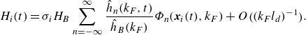 \begin{equation} H_i(t) = \sigma _iH_B \sum _{n = -\infty }^\infty \frac {\hat {h}_n(k_F, t)}{\hat {h}_B(k_F)}\varPhi _n(\boldsymbol{x}_{\kern-1pt i}(t), k_F) + O\big ((k_F l_d)^{-1}\big). \end{equation}
Finally, by differentiating (2.13c ) with respect to time and using (E5) and (E6), we deduce the leading-order wave energy evolution equation:
 \begin{equation} \frac {\mathrm {d} {E}}{\mathrm {d} {t}} = \frac {2E_B}{T_M}\left (\sum _{j = 1}^N\frac {H_j(t)}{H_B} - \frac {E(t)}{E_B}\right), \end{equation}
which is the multiple-droplet analogue of (2.17), valid in the high-memory limit.
For steady and slowly varying configurations, such as lattices (Eddi et al. Reference Eddi, Decelle, Fort and Couder2009; Couchman et al. Reference Couchman and Bush2022), rings (Couchman & Bush Reference Couchman and Bush2020; Thomson et al. Reference Thomson, Couchman and Bush2020a ) or orbiting pairs (Protière et al. Reference Protière, Boudaoud and Couder2006; Oza et al. Reference Oza, Siéfert, Harris, Moláček and Bush2017), we deduce from (E4) that the local wave height satisfies
 \begin{equation} H_i = H_B\bigg(\gamma _D(|\dot {\boldsymbol{x}}_{\kern-1pt i}|) + \sum _{j \neq i} \sigma _i\sigma _j \mathscr {H}\,(|\boldsymbol{x}_{\kern-1pt i} - {\boldsymbol{x\!}}_j|)\bigg), \end{equation}
and so depends on both the droplet speed (via the diminution factor,
 $\gamma _D$
) and the interaction potential, as is mediated by the accompanying Faraday wave field. Furthermore, it follows from (E7) that the wave energy is proportional to the mean wave height beneath the droplets, as expressed in (5.1), which represents the extension of (3.1) to multiple droplets. We thus deduce that the mean gravitational potential energy of droplets in a slowly evolving lattice may be treated as a proxy for wave energy. Finally, similar deductions may be made for periodic and quasi-periodic dynamical states of multiple droplets, including promenading pairs (Borghesi et al. Reference Borghesi, Moukhtar, Labousse, Eddi, Fort and Couder2014; Arbelaiz et al. Reference Arbelaiz, Oza and Bush2018), wobbling orbiting pairs (Oza et al. Reference Oza, Siéfert, Harris, Moláček and Bush2017) or various ring oscillations (Couchman & Bush Reference Couchman and Bush2020; Thomson et al. Reference Thomson, Couchman and Bush2020a
, Reference Thomson, Durey and Rosales2021), on the basis of results akin to those derived in § 3.
$\gamma _D$
) and the interaction potential, as is mediated by the accompanying Faraday wave field. Furthermore, it follows from (E7) that the wave energy is proportional to the mean wave height beneath the droplets, as expressed in (5.1), which represents the extension of (3.1) to multiple droplets. We thus deduce that the mean gravitational potential energy of droplets in a slowly evolving lattice may be treated as a proxy for wave energy. Finally, similar deductions may be made for periodic and quasi-periodic dynamical states of multiple droplets, including promenading pairs (Borghesi et al. Reference Borghesi, Moukhtar, Labousse, Eddi, Fort and Couder2014; Arbelaiz et al. Reference Arbelaiz, Oza and Bush2018), wobbling orbiting pairs (Oza et al. Reference Oza, Siéfert, Harris, Moláček and Bush2017) or various ring oscillations (Couchman & Bush Reference Couchman and Bush2020; Thomson et al. Reference Thomson, Couchman and Bush2020a
, Reference Thomson, Durey and Rosales2021), on the basis of results akin to those derived in § 3.


 Open access