1. Introduction
In recent years, more and more industrial robots have been applied to modern manufacturing systems. They are now fast and smooth with increased precision. However, in order to ensure high productivity and quality, they should be devised even more precisely. For this, trajectory planning for industrial robots is aimed to generate a desired smooth motion with high speed and precision under kinematical and geometrical constraints. In particular, smoothness in motion is essentially required in the delicate industrial setting such as spot-welding or precise assembly, where it is important that the planned trajectories should be continuous within the capability of actuators [Reference Macfarlane and Croft1, Reference Zhao, Gao and Zhang2]. Also, the residual vibration is an important issue for high-speed and precise motions [Reference Huaizhong Li, Gong and Lin3, Reference Ghariblu and Korayem4]. A method based on jerk constraints was efficient for smooth trajectory planning, providing an indirect means to restrict the variation rate of the actuator torques [Reference Gasparetto and Zanotto5]. Jerk constraints are especially significant in reducing machine abrasion, position error and residual vibration [Reference Kyriakopoulos and Saridis6, Reference Zanotto, Gasparetto, Lanzutti, Boscariol and Vidoni7]. The snap as the derivative of jerk is also the important factor in controlling the trade-off between efficiency and smoothness [Reference Fang, Hu, Liu, Shao, Qi and Peng8]. The higher snap constraints result in a shorter execution time, while the smoothness is decreased. In contrast with this, the smaller snap constraints result in a longer execution time, while the smoothness is increased. Therefore, the jerk and snap constraints have to be reasonably chosen in due consideration of the state of the machinery, product precision, productivity and so on.
The planning methods with high-order polynomial are being used for the smooth jerk-limited trajectory planning. Acceleration profiles with high-order polynomial under velocity, acceleration and jerk limits were used for the trajectory planning of several mechanisms [Reference Boryga9, Reference Xiao, Du and Dong10]. Cubic NURBS curves were extensively used to define the trajectory [Reference Saravanan, Ramabalan and Balamurugan11, Reference Zhao and Guo12]. Huang et al. improved the smoothness of trajectory planning of robotic manipulator by using the 5th order B-spline [Reference Huang, Hu, Wu and Zeng13]. The third-order spline in the Cartesian space was combined with the septuple B-spline in the joint space to generate time-optimal and jerk-continuous trajectories [Reference Lie, Lai and Wu14]. The time-optimal Acc/Dec method for multiple segments was applied to five-axis machining in ref. [Reference Kornmaneesang and Chen15], where a quintic B-spline corner smoothing method was utilized to smoothen sharp corners in the toolpath. Boryga et al. proposed the planning method of trajectory motions for the 6 DOF manipulator, in which the acceleration profile with higher-order polynomial was determined by one coefficient [Reference Boryga and Graboś16]. Yue et al. achieved the point-to-point trajectory planning of flexible redundant robotic manipulators by using the quadrinomial and quantic polynomials [Reference Yue, Henrich, Xu and Tso17]. Wang et al. planned a near time-optimal trajectory by the fourth-order polynomial with the property of root multiplicity, in which the polynomial curve was determined by only one coefficient [Reference Wang, Wang, Huang, Zhao and Quan18]. Lee et al. proposed an optimization process for polynomial-function-based motion profiles to achieve fast movement with low vibration, where the higher-order continuous trajectory was realized by increasing the degree of the polynomial model [Reference Lee and Ha19]. Generally, all the displacement, velocity, acceleration, jerk trajectories made by higher-order polynomial or spline were continuous, but many coefficients should be determined to generate trajectories.
S-curve trajectory planning is widely introduced for generating jerk-constrained motions. An S-curve model ensures reduction of residual vibration and impulse and the smoothness of the trajectory by determining time periods reasonably. Biagiotti et al. presented a new optimization algorithm that assures the minimum possible duration of generalized S-curve trajectories compliant with kinematic limitations and capable of suppressing residual vibrations [Reference Biagiotti and Melchiorri20]. Jose et al. developed an S-curve velocity profile which presents an acceleration and deceleration stage smoother than the trapezoidal velocity profile [Reference García-Martínez, Rodríguez-Reséndiz and Cruz-Miguel21]. Ni et al. proposed a novel bidirectional adaptive feedrate scheduling method based on S-shaped acceleration/deceleration algorithm [Reference Ni, Zhang, Ji, Hu, Chen, Liu and Wnag22]. The third-order polynomial S-curve trajectories for point-to-point motions were proposed, which became one of the widely used models [Reference Mu, Zhou, Yan and Han23, Reference Lu and Chen24]. Hassan et al. generated time-optimal pick-and-throw S-curve trajectories, which was based on a third-order polynomial model [Reference Hassan, Gouttefarde, Chemori, Herve, Rafei, Francis and Salle25]. The fourth-order polynomial S-curve model was proposed to eliminate the effect of harmful jerk such as impulse and residual vibration [Reference Chen, Wei, Sun, Liu and Wang26, Reference Song, Yu, Chen and Sun27]. Li et al. proposed the S-curve trajectory for which Acc/Dec profile was derived from the sinusoidal jerk function [Reference Huaizhong Li and Wei Lin28]. Also, Fang et al. proposed a methodology to generate online smooth joint trajectories of robots based on an improved sinusoidal jerk model [Reference Fang, Qi, Hu, Wang and Peng29]. Perumaal et al. generated the trigonometric S-curve trajectory with jerk constraint for the 6 DOF manipulator [Reference Perumaal and Jawahar30]. Fang et al. proposed the smooth and time-optimal trajectory planning, in which the piecewise sigmoid function was used for generating the jerk profile [Reference Fang, Hu, Liu, Shao, Qi and Peng8]. A symmetric S-curve trajectory has symmetric acceleration and deceleration stages. Therefore, the smaller jerk and the longer travelling time are needed to reduce the residual vibration effectively in the deceleration stage as well as in the acceleration stage. Therefore, the longer travelling time is needed to generate the smoother motion profile. To meet the requirement of the moving distance and travelling time simultaneously, the asymmetric profile was adopted [Reference Zou, Qu, Wang and Xu31, Reference Li, Liu and Sun32].
Recently, asymmetric trajectories have been presented in several papers to reduce the residual vibration and the settling time. In the asymmetric model, the requirements such as the time optimality and the reduction of the residual vibration can be achieved by making trajectories more aggressive in the acceleration stage and smoother in the deceleration stage. Bai et al. proposed a method for planning an asymmetric S-curve trajectory to reduce the residual vibration [Reference Bai, Chen, Sun and Yang33]. Li et al. proposed the time-optimal general asymmetric S-curve profile, which was capable of reducing the residual vibration more significantly than the traditional symmetric S-curve [Reference Li, Gao, Xiao, Cheng, Zhang and Hao34]. The asymmetric S-curve trajectory derived from the trigonometric jerk function was presented [Reference Li35]. Xin and Le proposed a method for planning an asymmetric S-type model using the dichotomy iteration and demonstrated that the asymmetric curve had considerable advantages over the symmetric S-curve model [Reference Li and Chen36]. Wu et al. improved the motion efficiency of industrial robots using a point-to-point trajectory planning based on a locally asymmetrical jerk profile, where the jerk motion profile was derived from the sinus function [Reference Wu, Chen, Bao, Wang, Zhang and Xu37]. Liu et al. presented the method planning the time-optimal asymmetric S-curve trajectory of redundant manipulators under kinematic constraints to design an end-effector motion profile along a specified path [Reference Liu, Cui, Li, Gao, Zhu and Chen38]. Most asymmetric models are based on the conventional symmetric S-curve profile [Reference Li, Gao, Xiao, Cheng, Zhang and Hao34, Reference Chettibi, Lehtihet, Haddad and Hanchi39].
In this paper, the symmetric S-curve model proposed in ref. [Reference Fang, Hu, Liu, Shao, Qi and Peng8] is expanded to an asymmetric one, which will make it possible to minimize the execution time as well as to achieve the smoother trajectory generation in the deceleration stage by decreasing the jerk in the deceleration stage and selecting the asymmetric parameter properly. The aim of this research is to develop a method of planning a new asymmetric S-curve trajectory for improving the smoothness and effectiveness of the motion. To do this, we generate a new asymmetric jerk profile by introducing an asymmetric parameter in the piecewise sigmoid function in the deceleration stage. Then, two analytic algorithms are presented, where one is to decide the time intervals of trajectory satisfying the time optimality under the kinematic constraints and the other is to select the asymmetric parameter for achieving the minimum execution time of motion.
The rest of this paper is presented as follows: Section 2 gives a trajectory planning method based on the improved jerk profile. The simulations of the 3 DOF and 6 DOF robotic manipulators are given in Section 3. The conclusion is drawn in Section 4.
2. Asymmetric S-Curve Trajectory Planning
2.1. Improved jerk profile model
A symmetric jerk profile was proposed by Fang et al. to reduce the complexity of calculation caused by the conventional high-order polynomial models and achieve more effective smoothness than trigonometric models [Reference Fang, Hu, Liu, Shao, Qi and Peng8]. Fig. 1 shows the kinematic profiles for the normal case of the model proposed in ref. [Reference Fang, Hu, Liu, Shao, Qi and Peng8].
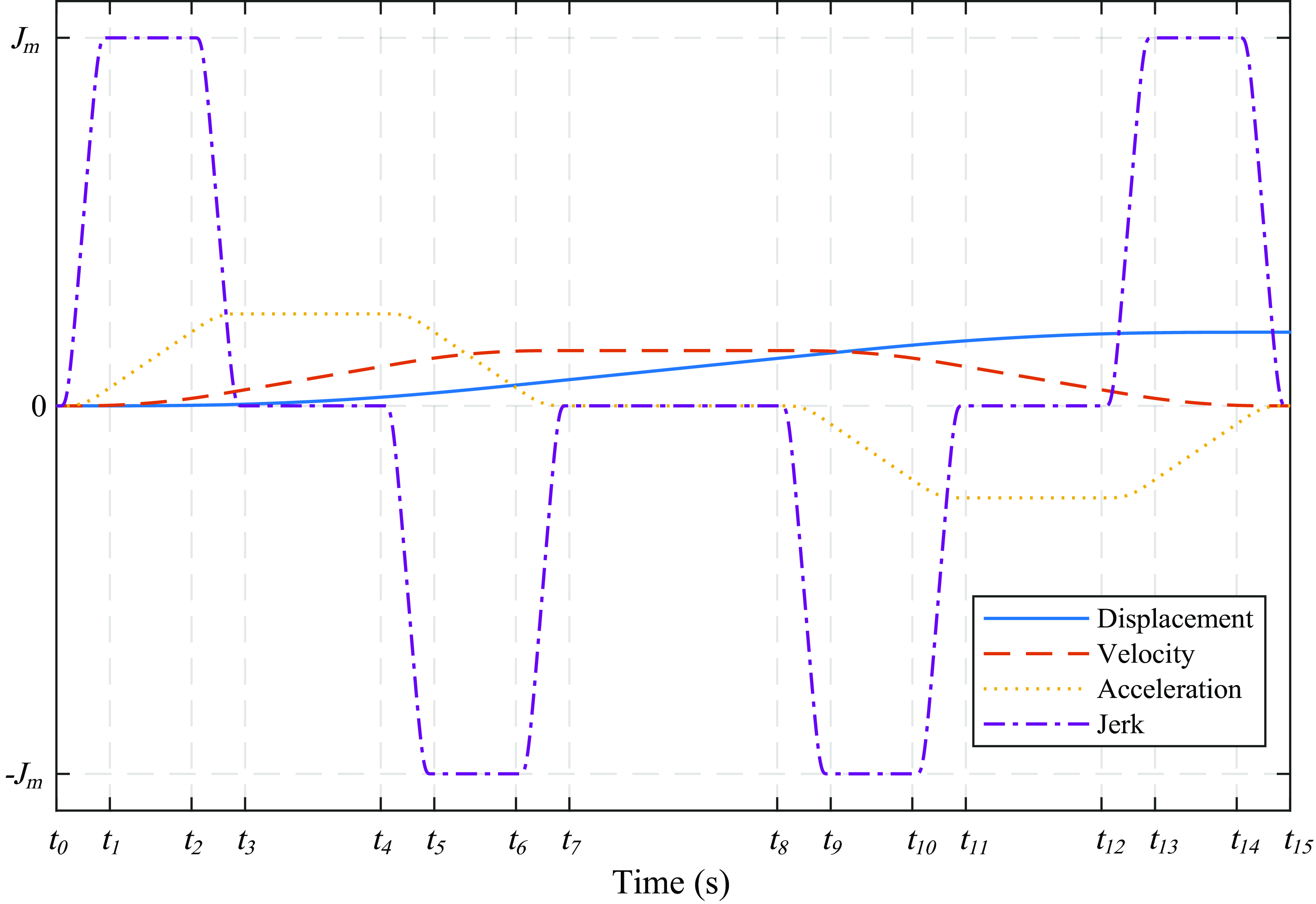
Figure 1. Kinematic profiles for the normal case of piecewise sigmoid S-curve model [Reference Fang, Hu, Liu, Shao, Qi and Peng8].
The jerk profile was defined as follows:
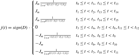 \begin{equation} j\!\left(t\right)=sign\!\left(D\right)\cdot \left\{\begin{array}{l@{\quad}l} J_{m}\frac{1}{1+e^{-\xi \!\left(1/\left(1-{\beta _{i}}\right)-1/{\beta _{i}}\right)}} & t_{0}\leq t\lt t_{1},\,t_{12}\leq t\lt t_{13}\\[5pt] J_{m} & t_{1}\leq t\lt t_{2},\,t_{13}\leq t\lt t_{14}\\[5pt] J_{m}\frac{1}{1+e^{\xi \left(1/\left(1-{\beta _{i}}\right)-1/{\beta _{i}}\right)}} & t_{2}\leq t\lt t_{3},\,t_{14}\leq t\lt t_{15}\\[5pt] 0 & t_{3}\leq t\lt t_{4},\,t_{7}\leq t\lt t_{8},t_{11}\leq t\lt t_{12}\\[5pt] -J_{m}\frac{1}{1+e^{-\xi \left(1/\left(1-{\beta _{i}}\right)-1/{\beta _{i}}\right)}} & t_{4}\leq t\lt t_{5},\,t_{8}\leq t\lt t_{9}\\[5pt] -J_{m} & t_{5}\leq t\lt t_{6},\,t_{9}\leq t\lt t_{10}\\[5pt] -J_{m}\frac{1}{1+e^{\xi \left(1/\left(1-{\beta _{i}}\right)-1/{\beta _{i}}\right)}} & t_{6}\leq t\lt t_{7},\,t_{10}\leq t\lt t_{11} \end{array}\right. \end{equation}
where
![]() $t_{i}\,(i=0,1,2,\cdots,15)$
is the initial time instant of the corresponding segment;
$t_{i}\,(i=0,1,2,\cdots,15)$
is the initial time instant of the corresponding segment;
![]() $\beta _{i}=(t-t_{i-1})/(t_{i}-t_{i-1})(i=1,3,5,\,\cdots,15)$
is the normalized variable in time period of
$\beta _{i}=(t-t_{i-1})/(t_{i}-t_{i-1})(i=1,3,5,\,\cdots,15)$
is the normalized variable in time period of
![]() $[t_{i-1},t_{i}];\;\xi$
is the positive constant corresponding to the variation rate and
$[t_{i-1},t_{i}];\;\xi$
is the positive constant corresponding to the variation rate and
![]() $D$
is the relative displacement from the initial position that can be either positive or negative.
$D$
is the relative displacement from the initial position that can be either positive or negative.
As shown in Fig. 1, the kinematic profiles for velocity, acceleration and jerk in the acceleration and deceleration stages exhibit the symmetry for the point-to-point motion. They are continuous and infinitely differentiable under the kinematic constraints. For point-to-point trajectory planning, it is important to effectively reduce the residual vibration in the vicinity of the target point in the minimum execution time. To this end, the trajectories in the acceleration stage can be more aggressive, while those in the deceleration stage can be smoother. From this point of view, we expanded the symmetric jerk profile in ref. [Reference Fang, Hu, Liu, Shao, Qi and Peng8] to an asymmetric profile. The asymmetric jerk profile is defined as follows:
 \begin{equation} j\!\left(t\right)=sign\!\left(D\right)\cdot \left\{\begin{array}{l@{\quad}l} J_{m}\frac{1}{1+e^{-\xi \left(1/\left(1-{\beta _{1}}\right)-1/{\beta _{1}}\right)}} & t_{0}\leq t\lt t_{1}\\[5pt] J_{m} & t_{1}\leq t\lt t_{2}\\[5pt] J_{m}\frac{1}{1+e^{\xi \left(1/\left(1-{\beta _{3}}\right)-1/{\beta _{3}}\right)}} & t_{2}\leq t\lt t_{3}\\[5pt] 0 & t_{3}\leq t\lt t_{4}\\[5pt] -J_{m}\frac{1}{1+e^{-\xi \left(1/\left(1-{\beta _{5}}\right)-1/{\beta _{5}}\right)}} & t_{4}\leq t\lt t_{5}\\[5pt] -J_{m} & t_{5}\leq t\lt t_{6}\\[5pt] -J_{m}\frac{1}{1+e^{\xi \left(1/\left(1-{\beta _{7}}\right)-1/{\beta _{7}}\right)}} & t_{6}\leq t\lt t_{7}\\[5pt] 0 & t_{7}\leq t\lt t_{8}\\[5pt] -J_{m}\frac{\lambda }{1+e^{-\xi \left(1/\left(1-{\beta _{9}}\right)-1/{\beta _{9}}\right)}} & t_{8}\leq t\lt t_{9}\\[5pt] -\lambda J_{m} & t_{9}\leq t\lt t_{10}\\[5pt] -J_{m}\frac{\lambda }{1+e^{\xi \left(1/\left(1-{\beta _{11}}\right)-1/{\beta _{11}}\right)}} & t_{10}\leq t\lt t_{11}\\[5pt] 0 & t_{11}\leq t\lt t_{12}\\[5pt] J_{m}\frac{\lambda }{1+e^{-\xi \left(1/\left(1-{\beta _{13}}\right)-1/{\beta _{13}}\right)}} & t_{12}\leq t\lt t_{13}\\[5pt] \lambda J_{m} & t_{13}\leq t\lt t_{14}\\[5pt] J_{m}\frac{\lambda }{1+e^{\xi \left(1/\left(1-{\beta _{15}}\right)-1/{\beta _{15}}\right)}} & t_{14}\leq t\lt t_{15} \end{array}\right. \end{equation}
where
![]() $J_{m}$
is the maximum jerk in the acceleration stage;
$J_{m}$
is the maximum jerk in the acceleration stage;
![]() $\lambda$
is the asymmetric parameter (
$\lambda$
is the asymmetric parameter (
![]() $0\lt \lambda \leq 1$
);
$0\lt \lambda \leq 1$
);
![]() $\xi$
is the positive coefficient; and
$\xi$
is the positive coefficient; and
![]() $\beta _{i}=(t-t_{i-1})/(t_{i}-t_{i-1})$
. The kinematic profiles for the normal case are illustrated in Fig. 2, where
$\beta _{i}=(t-t_{i-1})/(t_{i}-t_{i-1})$
. The kinematic profiles for the normal case are illustrated in Fig. 2, where
![]() $V_{m},\, A_{m}$
and
$V_{m},\, A_{m}$
and
![]() $J_{m}$
denote the maximum allowable velocity, acceleration and jerk, respectively.
$J_{m}$
denote the maximum allowable velocity, acceleration and jerk, respectively.
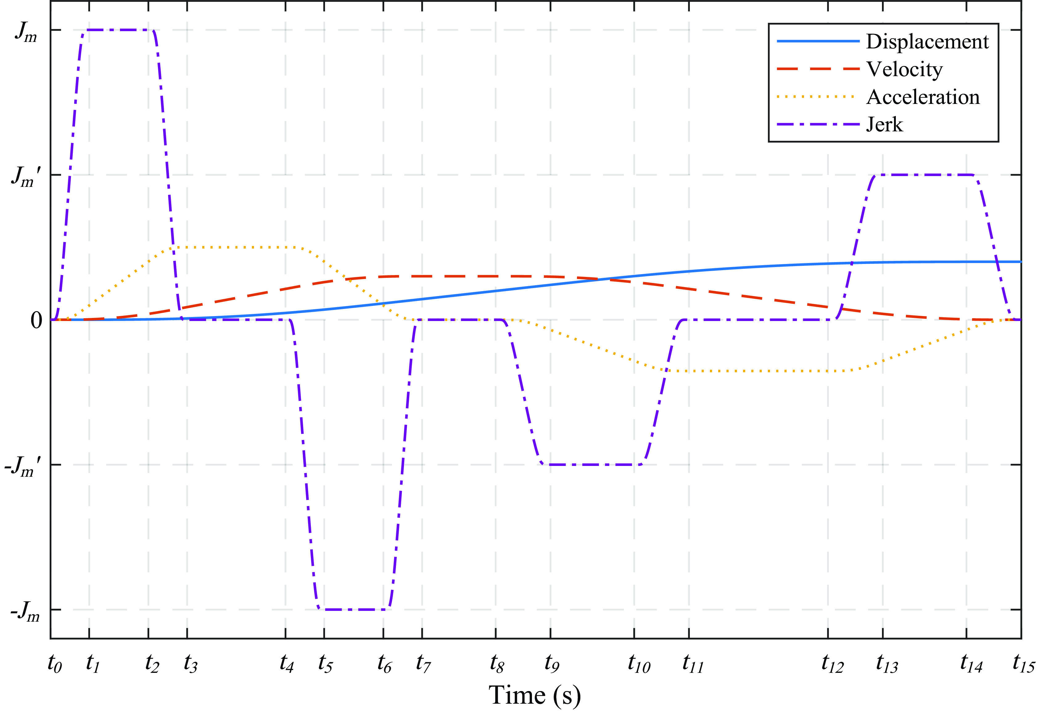
Figure 2. Kinematic profiles for the normal case of the proposed asymmetric S-curve models.
Eq. (2) allows the jerk to vary smoothly between 0 and the maximum allowable value so that the generated trajectories can be infinitely differentiable. The trajectory consists of fifteen segments, whose time interval is denoted as
![]() $I_{i}=t_{i}-t_{i-1}(i=1,2,\,\cdots,15)$
.
$I_{i}=t_{i}-t_{i-1}(i=1,2,\,\cdots,15)$
.
As shown in Fig. 2, the idea of the asymmetric profile is to decrease as much as possible the maximum allowable jerk in the deceleration stage without affecting the acceleration stage. Thus, the maximum allowable jerk in the acceleration stage is determined by the maximum capability of the actuator, while the maximum allowable jerk in the deceleration stage can be defined manually, or with the purpose of satisfying the minimum execution time.
![]() $I_{1}=I_{3}=I_{5}=I_{7}$
and
$I_{1}=I_{3}=I_{5}=I_{7}$
and
![]() $I_{2}=I_{6}$
are set for the acceleration stage
$I_{2}=I_{6}$
are set for the acceleration stage
![]() $[t_{0,}t_{7}]$
to have the null acceleration at the time instant of
$[t_{0,}t_{7}]$
to have the null acceleration at the time instant of
![]() $t_{7}$
. Correspondingly, the deceleration stage
$t_{7}$
. Correspondingly, the deceleration stage
![]() $[t_{8,}t_{15}]$
has
$[t_{8,}t_{15}]$
has
![]() $I_{9}=I_{11}=I_{13}=I_{15}$
and
$I_{9}=I_{11}=I_{13}=I_{15}$
and
![]() $I_{10}=I_{14}$
. The shape of trajectory depends on the actual maximum jerks in the acceleration and deceleration stages. Moreover, it also depends on seven time intervals, which are composed of the varying jerk intervals
$I_{10}=I_{14}$
. The shape of trajectory depends on the actual maximum jerks in the acceleration and deceleration stages. Moreover, it also depends on seven time intervals, which are composed of the varying jerk intervals
![]() $I_{s}$
and
$I_{s}$
and
![]() $I^{\prime}_{s}$
, the constant jerk intervals
$I^{\prime}_{s}$
, the constant jerk intervals
![]() $I_{j}$
and
$I_{j}$
and
![]() $I^{\prime}_{j}$
, the constant acceleration intervals
$I^{\prime}_{j}$
, the constant acceleration intervals
![]() $I_{a}$
and
$I_{a}$
and
![]() $I^{\prime}_{a}$
, and the constant velocity interval
$I^{\prime}_{a}$
, and the constant velocity interval
![]() $I_{v}$
. Then, the total execution time
$I_{v}$
. Then, the total execution time
![]() $I_{\textit{total}}$
is the sum of the time intervals of all the fifteen phases:
$I_{\textit{total}}$
is the sum of the time intervals of all the fifteen phases:
![]() $I_{\textit{total}}=\sum _{i=1}^{15}I_{i}=4(I_{s}+I^{\prime}_{s})+2(I_{j}+I^{\prime}_{j})+I_{a}+I^{\prime}_{a}+I_{v}$
.
$I_{\textit{total}}=\sum _{i=1}^{15}I_{i}=4(I_{s}+I^{\prime}_{s})+2(I_{j}+I^{\prime}_{j})+I_{a}+I^{\prime}_{a}+I_{v}$
.
The objective of the asymmetric S-curve trajectory planning is to calculate the time intervals
![]() $I_{s},\,I^{\prime}_{s},\,I_{j},\,I^{\prime}_{j},\,I_{a},\,I^{\prime}_{a}$
and
$I_{s},\,I^{\prime}_{s},\,I_{j},\,I^{\prime}_{j},\,I_{a},\,I^{\prime}_{a}$
and
![]() $I_{v}$
to optimize the total execution time under the given kinematic constraints. Acceleration
$I_{v}$
to optimize the total execution time under the given kinematic constraints. Acceleration
![]() $a(t)$
, velocity
$a(t)$
, velocity
![]() $v(t)$
and displacement functions
$v(t)$
and displacement functions
![]() $d(t)$
cannot be given analytically, for it is impossible to integrate this jerk function. However, the values of these kinematic variables at every connection time instant can be numerically calculated as the area values under the curve of their derivatives. When the trajectory consists of fifteen segments as shown in Fig. 2, the following relationships between the kinematic values and time intervals hold:
$d(t)$
cannot be given analytically, for it is impossible to integrate this jerk function. However, the values of these kinematic variables at every connection time instant can be numerically calculated as the area values under the curve of their derivatives. When the trajectory consists of fifteen segments as shown in Fig. 2, the following relationships between the kinematic values and time intervals hold:
 \begin{equation} \left\{\begin{array}{l} A_{m}=a\!\left(t_{3}\right)=a\!\left(t_{4}\right)=J_{m}\!\left(I_{s}+I_{j}\right)\\[5pt] A^{\prime}_{m}=a\!\left(t_{11}\right)=a\!\left(t_{12}\right)=J^{\prime}_{m}\!\left(I^{\prime}_{s}+I^{\prime}_{j}\right)\\[5pt] V_{m}=v\!\left(t_{7}\right)=v\!\left(t_{8}\right)=A_{m}\!\left(2I_{s}+I_{j}+I_{a}\right)=A^{\prime}_{m}\!\left(2I^{\prime}_{s}+I^{\prime}_{j}+I^{\prime}_{a}\right)\\[5pt] \left| D\right| =\left| d\!\left(15\right)\right| =V_{m}\!\left[2\!\left(I_{s}+I^{\prime}_{s}\right)+I_{j}+I^{\prime}_{j}+\frac{1}{2}\!\left(I_{a}+I^{\prime}_{a}\right)+I_{v}\right] \end{array}\right. \end{equation}
where
![]() $V_{m},\,A_{m}$
and
$V_{m},\,A_{m}$
and
![]() $J_{m}$
are the maximum allowable values within the capability of the actuator,
$J_{m}$
are the maximum allowable values within the capability of the actuator,
![]() $A^{\prime}_{m}$
and
$A^{\prime}_{m}$
and
![]() $J^{\prime}_{m}$
are the maximum allowable acceleration and jerk in the deceleration stage, and
$J^{\prime}_{m}$
are the maximum allowable acceleration and jerk in the deceleration stage, and
![]() $D$
is the travelling distance, representing the displacement relative to the initial and the final position that can be either positive or negative.
$D$
is the travelling distance, representing the displacement relative to the initial and the final position that can be either positive or negative.
The maximum allowable jerk in the deceleration stage is given as follows:
Considering the smoothness of deceleration stage,
![]() $\lambda$
is set to be less than 1. In order to achieve the complete closed-form solutions for this asymmetric trajectory, let us assume the relationships between the corresponding time intervals of the acceleration and deceleration stages as follows:
$\lambda$
is set to be less than 1. In order to achieve the complete closed-form solutions for this asymmetric trajectory, let us assume the relationships between the corresponding time intervals of the acceleration and deceleration stages as follows:
By substituting Eq. (4) and Eq. (5) into Eq. (3), the following equation is derived:
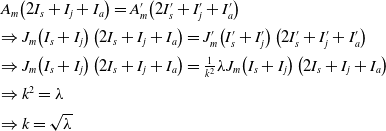 \begin{equation} \begin{array}{l} A_{m}\!\left(2I_{s}+I_{j}+I_{a}\right)=A^{\prime}_{m}\!\left(2I^{\prime}_{s}+I^{\prime}_{j}+I^{\prime}_{a}\right)\\[5pt] \Rightarrow J_{m}\!\left(I_{s}+I_{j}\right)\left(2I_{s}+I_{j}+I_{a}\right)=J^{\prime}_{m}\!\left(I^{\prime}_{s}+I^{\prime}_{j}\right)\left(2I^{\prime}_{s}+I^{\prime}_{j}+I^{\prime}_{a}\right)\\[5pt] \Rightarrow J_{m}\!\left(I_{s}+I_{j}\right)\left(2I_{s}+I_{j}+I_{a}\right)=\frac{1}{k^{2}}\lambda J_{m}\!\left(I_{s}+I_{j}\right)\left(2I_{s}+I_{j}+I_{a}\right)\\[5pt] \Rightarrow k^{2}=\lambda \\[5pt] \Rightarrow k=\sqrt{\lambda } \end{array} \end{equation}
If the above result is substituted into Eq. (5), then
 \begin{equation} \left\{\begin{array}{l} I^{\prime}_{s}=\frac{I_{s}}{\sqrt{\lambda }}\\[5pt] I^{\prime}_{j}=\frac{I_{j}}{\sqrt{\lambda }}\\[5pt] I^{\prime}_{a}=\frac{I_{a}}{\sqrt{\lambda }} \end{array}\right. \end{equation}
Fang et al. [Reference Fang, Hu, Liu, Shao, Qi and Peng8] decided
![]() $\xi =\sqrt{3}/2$
in Eq. (1) under the assumption that the maximum snap should be as small as possible when the execution time and jerk constraints are constant. In the proposed method,
$\xi =\sqrt{3}/2$
in Eq. (1) under the assumption that the maximum snap should be as small as possible when the execution time and jerk constraints are constant. In the proposed method,
![]() $\xi =\sqrt{3}/2$
is used. Then, in the case that the maximum snap in the acceleration stage is constrained by the given
$\xi =\sqrt{3}/2$
is used. Then, in the case that the maximum snap in the acceleration stage is constrained by the given
![]() $S_{m}$
, the relationship between
$S_{m}$
, the relationship between
![]() $S_{m}$
and the actual maximum jerk is defined as:
$S_{m}$
and the actual maximum jerk is defined as:
Similarly, it is also defined as
![]() $j^{\prime}_{m}=S^{\prime}_{m}I^{\prime}_{s}/\sqrt{3}$
in the deceleration stage.
$j^{\prime}_{m}=S^{\prime}_{m}I^{\prime}_{s}/\sqrt{3}$
in the deceleration stage.
Because the snap has the direct interrelation with the jerk varying period, then the trade-off between the time optimality and the smoothness can be controlled by
![]() $S_{m}$
.
$S_{m}$
.
 \begin{equation} \begin{array}{l} \lambda =\frac{j^{\prime}_{m}}{j_{m}}=\frac{\frac{S^{\prime}_{m}I^{\prime}_{s}}{\sqrt{3}}}{\frac{S_{m}I_{s}}{\sqrt{3}}}=\frac{S^{\prime}_{m}I^{\prime}_{s}}{S_{m}I_{s}}=\frac{S^{\prime}_{m}}{kS_{m}}=\frac{S^{\prime}_{m}}{\sqrt{\lambda }S_{m}}\\[9pt] \Rightarrow S^{\prime}_{m}=\lambda ^{\frac{3}{2}}S_{m} \end{array} \end{equation}
The other actual maximum kinematic values can be written as:
 \begin{equation} \left\{\begin{array}{l} a_{m}=\frac{S_{m}I_{s}}{\sqrt{3}}\left(I_{s}+I_{j}\right)\\[5pt] a^{\prime}_{m}=\frac{S^{\prime}_{m}I^{\prime}_{s}}{\sqrt{3}}\left(I^{\prime}_{s}+I^{\prime}_{j}\right)\\[5pt] v_{m}=\frac{S_{m}I_{s}}{\sqrt{3}}\left(I_{s}+I_{j}\right)\left(2I_{s}+I_{j}+I_{a}\right)=\frac{S^{\prime}_{m}I^{\prime}_{s}}{\sqrt{3}}\left(I^{\prime}_{s}+I^{\prime}_{j}\right)\left(2I^{\prime}_{s}+I^{\prime}_{j}+I^{\prime}_{a}\right)\\[5pt] d_{m}=\frac{S_{m}I_{s}}{\sqrt{3}}\left(I_{s}+I_{j}\right)\left(2I_{s}+I_{j}+I_{a}\right)\left[2\!\left(I_{s}+I^{\prime}_{s}\right)+I_{j}+I^{\prime}_{j}+\frac{1}{2}\left(I_{a}+I^{\prime}_{a}\right)+I_{v}\right] \end{array}\right. \end{equation}
Substituting Eq. (7) into Eq. (10), Eq. (11) is obtained.
 \begin{equation} \left\{\begin{array}{l} a_{m}=\frac{S_{m}I_{s}}{\sqrt{3}}\left(I_{s}+I_{j}\right)\\[5pt] a^{\prime}_{m}=\sqrt{\frac{\lambda }{3}}S_{m}I_{s}\!\left(I_{s}+I_{j}\right)\\[5pt] v_{m}=\frac{S_{m}I_{s}}{\sqrt{3}}\left(I_{s}+I_{j}\right)\left(2I_{s}+I_{j}+I_{a}\right)\\[5pt] d_{m}=\frac{S_{m}I_{s}}{\sqrt{3}}\left(I_{s}+I_{j}\right)\left(2I_{s}+I_{j}+I_{a}\right)\left[\left(1+\frac{1}{\sqrt{\lambda }}\right)\left(2I_{s}+I_{j}+\frac{1}{2}I_{a}\right)+I_{v}\right] \end{array}\right. \end{equation}
Once the time intervals in the acceleration stage are determined, the corresponding values of the deceleration stage are obtained by them from Eq. (8), Eq. (10) and Eq. (11). Hence, in the following subsection, the time intervals in the acceleration stage are calculated to obtain the optimal execution time of the motion.
2.2. Calculation of time intervals
There exists no systematic method to find a time-optimal value for S-curve trajectory planning under the kinematic constraints. In the practical applications, the time intervals
![]() $I_{j}, I_{a}$
and
$I_{j}, I_{a}$
and
![]() $I_{v}$
may exist or not for achieving the optimal execution time under the target displacement and the kinematic limits. Only the jerk varying interval
$I_{v}$
may exist or not for achieving the optimal execution time under the target displacement and the kinematic limits. Only the jerk varying interval
![]() $I_{s}$
exists in generating the trajectory. All possible cases can be divided into eight types. In order to obtain the case with optimal execution time out of eight cases, four steps are set below. Figs. 3-4 show the flowchart of algorithm and all the possible jerk profiles.
$I_{s}$
exists in generating the trajectory. All possible cases can be divided into eight types. In order to obtain the case with optimal execution time out of eight cases, four steps are set below. Figs. 3-4 show the flowchart of algorithm and all the possible jerk profiles.
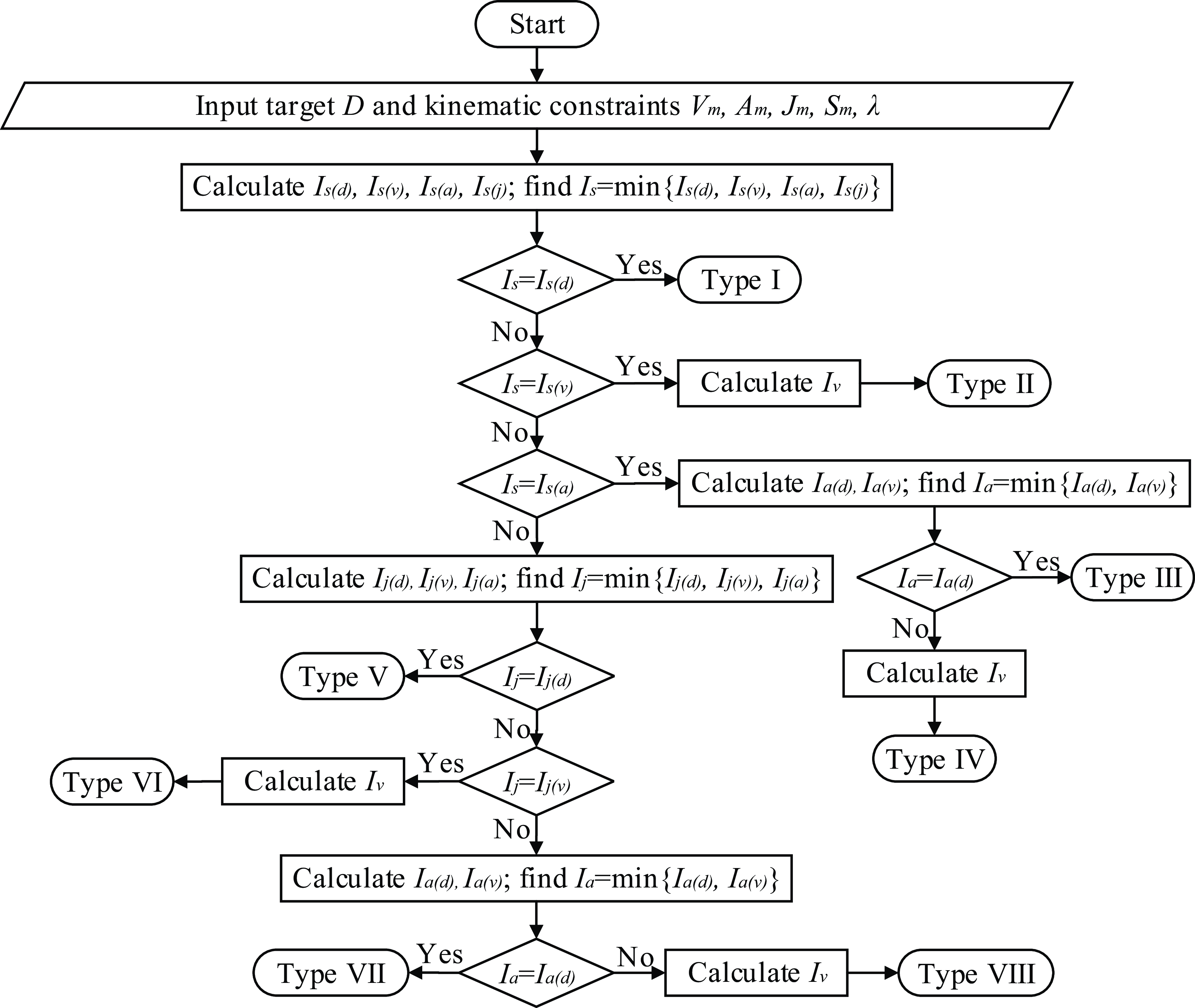
Figure 3. Calculation flowchart of algorithm.
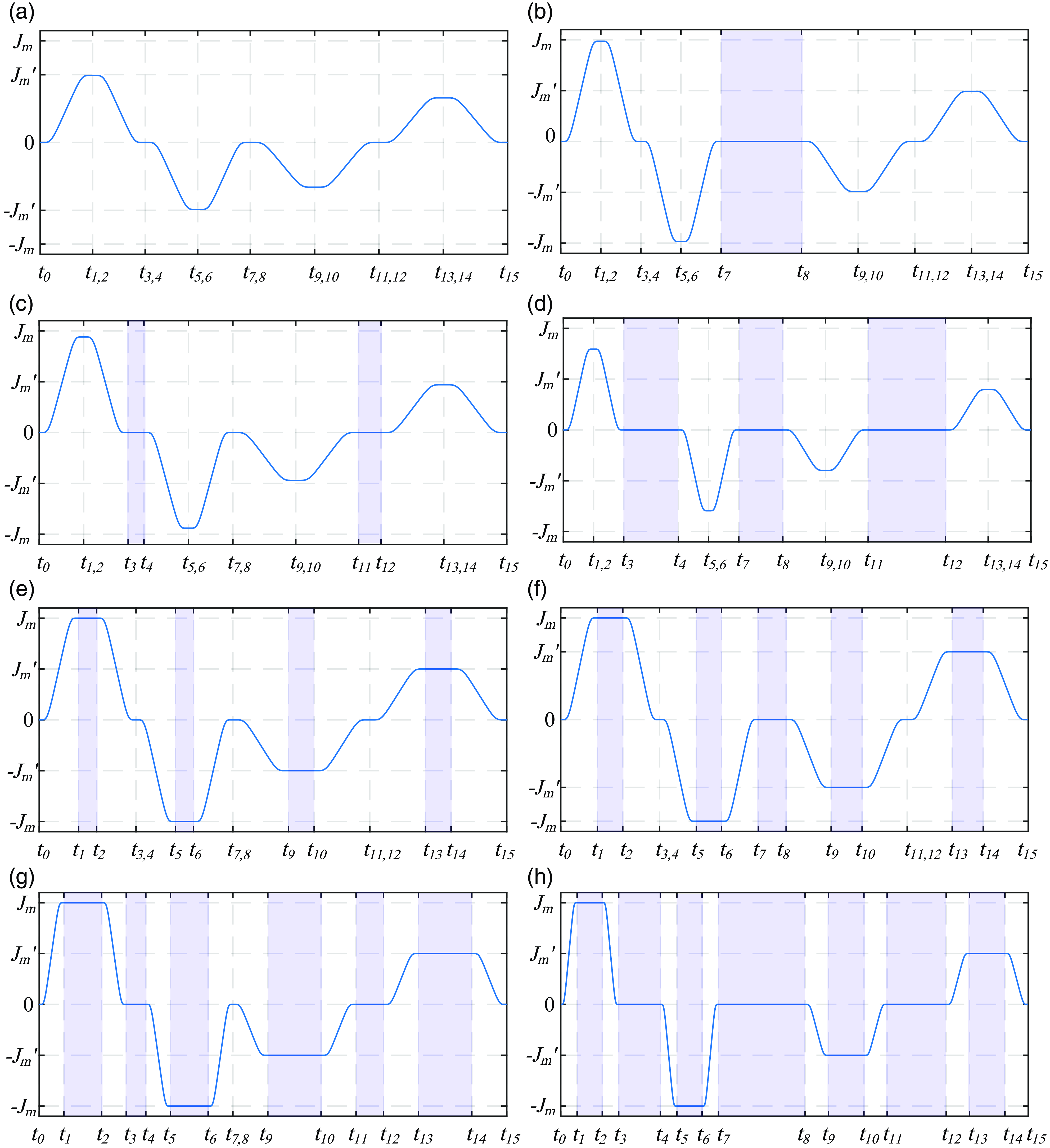
Figure 4. Jerk profile models: (a) Type I; (b) Type II; (c) Type III; (d) Type IV; (e) Type V; (f) Type VI; (g) Type VII; (h) Type VIII.
Step 1: Determination of the varying jerk interval
![]() $I_{s}$
$I_{s}$
(I) Firstly, the relationship between the target distance
![]() $d(t_{15})$
with the specific limit of snap,
$d(t_{15})$
with the specific limit of snap,
![]() $S_{m}$
and the time interval
$S_{m}$
and the time interval
![]() $I_{s}$
is established from Eq. (13) under the assumption without exceeding the constraints of jerk, acceleration and velocity.
$I_{s}$
is established from Eq. (13) under the assumption without exceeding the constraints of jerk, acceleration and velocity.
This includes that
![]() $I_{j}, I_{a}$
and
$I_{j}, I_{a}$
and
![]() $I_{v}$
don’t exist.
$I_{v}$
don’t exist.
 \begin{equation} d_{m}=\left| d\!\left(t_{15}|I_{j}=I_{a}=I_{v}=0\right)\right| =\frac{4\!\left(1+\frac{1}{\sqrt{\lambda }}\right)S_{m}I_{s}^{4}}{\sqrt{3}} \end{equation}
To obtain the target distance, the left side is set to be
![]() $D$
and the additional subscript is added to distinguish the values of
$D$
and the additional subscript is added to distinguish the values of
![]() $I_{s}$
calculated with the different constraints below. Then
$I_{s}$
calculated with the different constraints below. Then
![]() $I_{s}$
decided by the displacement is as follows:
$I_{s}$
decided by the displacement is as follows:
 \begin{equation} I_{s\left(d\right)}=\sqrt[4]{\frac{\sqrt{3}\left| D\right| }{4\!\left(1+\frac{1}{\sqrt{\lambda }}\right)S_{m}}} \end{equation}
This value can be broken by the given kinematic constraints and so it is essential to confirm the upper bound of
![]() $I_{s}$
related with them.
$I_{s}$
related with them.
(II) Then, the maximum velocity limit is introduced. It is clear that the maximum velocity is achieved at the time
![]() $t_{7}$
. That is,
$t_{7}$
. That is,
![]() $v_{m}$
should not be larger than the velocity constraint
$v_{m}$
should not be larger than the velocity constraint
![]() $V_{m}$
of the actuator and the limit of corresponding period
$V_{m}$
of the actuator and the limit of corresponding period
![]() $I_{s}$
is obtained as
$I_{s}$
is obtained as
 \begin{equation} I_{s\left(v\right)}=\sqrt[3]{\frac{\sqrt{3}V_{m}}{2S_{m}}} \end{equation}
(III) Next, the constraint of maximum acceleration should be considered. The acceleration reaches the maximum at the time
![]() $I_{s}$
.
$I_{s}$
.
Considering the acceleration constraint,
![]() $a_{m}$
sets to be
$a_{m}$
sets to be
![]() $A_{m}$
. Thus,
$A_{m}$
. Thus,
![]() $I_{s}$
is calculated as follows:
$I_{s}$
is calculated as follows:
 \begin{equation} I_{s\left(a\right)}=\sqrt{\frac{\sqrt{3}A_{m}}{S_{m}}} \end{equation}
(IV) Finally,
![]() $I_{s}$
constrained by jerk bound can be derived directly from Eq. (8).
$I_{s}$
constrained by jerk bound can be derived directly from Eq. (8).
![]() $I_{s}$
from Eq. (19) satisfies all constraints and is used in the rest steps.
$I_{s}$
from Eq. (19) satisfies all constraints and is used in the rest steps.
Then there exist four possible values for
![]() $I_{s}$
.
$I_{s}$
.
Case 1: If
![]() $I_{s(d)}=\min \{I_{s(d)},I_{s(v)},I_{s(a)},I_{s(j)}\}$
, the time interval existing during the motion is only the varying jerk interval and
$I_{s(d)}=\min \{I_{s(d)},I_{s(v)},I_{s(a)},I_{s(j)}\}$
, the time interval existing during the motion is only the varying jerk interval and
![]() $I_{j}=I_{a}=I_{v}=0$
. Then, the actual maximum velocity, acceleration, jerk and the total execution time are as Eq. (20) and complete to calculate.
$I_{j}=I_{a}=I_{v}=0$
. Then, the actual maximum velocity, acceleration, jerk and the total execution time are as Eq. (20) and complete to calculate.
Case 2: If
![]() $I_{s(v)}=\min \{I_{s(d)},I_{s(v)},I_{s(a)},I_{s(j)}\}$
, the actual maximum velocity is reached while the maximum acceleration and jerk aren’t reached. Thus
$I_{s(v)}=\min \{I_{s(d)},I_{s(v)},I_{s(a)},I_{s(j)}\}$
, the actual maximum velocity is reached while the maximum acceleration and jerk aren’t reached. Thus
![]() $I_{j}=I_{a}=0$
and the actual maximum jerk is calculated by Eq. (21). Go to step 4.
$I_{j}=I_{a}=0$
and the actual maximum jerk is calculated by Eq. (21). Go to step 4.
Case 3: If
![]() $I_{s(a)}=\min \{I_{s(d)},I_{s(v)},I_{s(a)},I_{s(j)}\}, I_{j}=0$
. The constant jerk interval disappears by the acceleration constraint. Then, the actual maximum jerk is calculated by Eq. (22). Go to step 3.
$I_{s(a)}=\min \{I_{s(d)},I_{s(v)},I_{s(a)},I_{s(j)}\}, I_{j}=0$
. The constant jerk interval disappears by the acceleration constraint. Then, the actual maximum jerk is calculated by Eq. (22). Go to step 3.
Case 4: If
![]() $I_{s(j)}=\min \{I_{s(d)},I_{s(v)},I_{s(a)},I_{s(j)}\}$
, the actual maximum jerk is equal to the maximum allowable jerk, that is
$I_{s(j)}=\min \{I_{s(d)},I_{s(v)},I_{s(a)},I_{s(j)}\}$
, the actual maximum jerk is equal to the maximum allowable jerk, that is
![]() $j_{m}=J_{m}$
. Then go to step 2.
$j_{m}=J_{m}$
. Then go to step 2.
Step 2: Determination of the constant jerk interval
![]() $I_{j}$
$I_{j}$
(I) Supposing that the acceleration and velocity constraints are satisfied, we start to calculate
![]() $I_{j}$
with the relationship between the final displacement and
$I_{j}$
with the relationship between the final displacement and
![]() $I_{j}$
.
$I_{j}$
.
 \begin{equation} \begin{array}{l} \left| d\!\left(t_{15}|I_{a}=I_{v}=0\right)\right| =\left| D\right| =j_{m}\!\left(4I_{s}^{3}+8I_{s}^{2}I_{j}+5I_{s}I_{j}^{2}+I_{j}^{3}\right)\left(1+\frac{1}{\sqrt{\lambda }}\right)\\[5pt] \Rightarrow I_{j\left(d\right)}=\sqrt[3]{\frac{I_{s}^{3}}{27}+\frac{\left| D\right| }{2\left(1+\frac{1}{\sqrt{\lambda }}\right)j_{m}}+\sqrt{\frac{\left| D\right| }{27\left(1+\frac{1}{\sqrt{\lambda }}\right)j_{m}}+\frac{D^{2}}{4\!\left(1+\frac{1}{\sqrt{\lambda }}\right)^{2}j_{m}^{2}}}}\\[5pt] +\sqrt[3]{\frac{I_{s}^{3}}{27}+\frac{\left| D\right| }{2\left(1+\frac{1}{\sqrt{\lambda }}\right)j_{m}}-\sqrt{\frac{\left| D\right| }{27\left(1+\frac{1}{\sqrt{\lambda }}\right)j_{m}}+\frac{D^{2}}{4\!\left(1+\frac{1}{\sqrt{\lambda }}\right)^{2}j_{m}^{2}}}}-\frac{5I_{s}}{3} \end{array} \end{equation}
Since
![]() $I_{s}$
and
$I_{s}$
and
![]() $j_{m}$
were decided in Step 1, from now on, we use
$j_{m}$
were decided in Step 1, from now on, we use
![]() $j_{m}$
instead of
$j_{m}$
instead of
![]() $S_{m}I_{s}/\sqrt{3}$
in Eq. (11).
$S_{m}I_{s}/\sqrt{3}$
in Eq. (11).
(II)
![]() $I_{j}$
under the velocity constraint is obtained as:
$I_{j}$
under the velocity constraint is obtained as:
 \begin{equation} \begin{array}{l} v\!\left(t_{7}|I_{a}=0\right)=V_{m}=j_{m}\!\left(2I_{s}^{2}+3I_{s}I_{j}+I_{j}^{2}\right)\\[5pt] \Rightarrow I_{j\left(v\right)}=-\frac{3I_{s}}{2}+\sqrt{\frac{I_{s}^{2}}{4}+\frac{V_{m}}{j_{m}}} \end{array} \end{equation}
(III)
![]() $I_{j}$
under the acceleration constraint is calculated as follows:
$I_{j}$
under the acceleration constraint is calculated as follows:
 \begin{equation} \begin{array}{l} a\!\left(t_{3}\right)=A_{m}=j_{m}\!\left(I_{j}+I_{s}\right)\\[5pt] \Rightarrow I_{j\left(a\right)}=-\frac{A_{m}}{j_{m}}-I_{s} \end{array} \end{equation}
Then, the constant jerk interval
![]() $I_{j}$
is selected by Eq. (26) and
$I_{j}$
is selected by Eq. (26) and
Then, there exists three possible values for
![]() $I_{j}$
.
$I_{j}$
.
Case 1: If
![]() $I_{j(d)}=\min \{I_{j(d)},\,I_{j(v)},\,I_{j(a)}\}, I_{a}=I_{v}=0$
. Then, the actual maximum velocity, acceleration and the total execution time are as Eq. (27) and complete to calculate.
$I_{j(d)}=\min \{I_{j(d)},\,I_{j(v)},\,I_{j(a)}\}, I_{a}=I_{v}=0$
. Then, the actual maximum velocity, acceleration and the total execution time are as Eq. (27) and complete to calculate.
 \begin{equation} \left\{\begin{array}{l} a_{m}=j_{m}\!\left(I_{s}+I_{j\left(d\right)}\right)\\[5pt] v_{m}=j_{m}\!\left(I_{s}+I_{j\left(d\right)}\right)\left(2I_{s}+I_{j\left(d\right)}\right)\\[5pt] I_{\textit{total}}=\left(4I_{s}+2I_{j\left(d\right)}\right)\left(1+1/\sqrt{\lambda }\right) \end{array}\right. \end{equation}
Case 2: If
![]() $I_{j(v)}=\min \{I_{j(d)},\,I_{j(v)},\,I_{j(a)}\}$
, then
$I_{j(v)}=\min \{I_{j(d)},\,I_{j(v)},\,I_{j(a)}\}$
, then
![]() $I_{a}=0$
. Therefore, the acceleration does not need to reach its maximum for achieving the maximum allowable velocity. Then, the actual maximum velocity and acceleration are given as Eq. (28) and go to Step 4.
$I_{a}=0$
. Therefore, the acceleration does not need to reach its maximum for achieving the maximum allowable velocity. Then, the actual maximum velocity and acceleration are given as Eq. (28) and go to Step 4.
 \begin{equation} \left\{\begin{array}{l} a_{m}=j_{m}\!\left(I_{s}+I_{j\left(v\right)}\right)\\[5pt] v_{m}=j_{m}\!\left(I_{s}+I_{j\left(v\right)}\right)\left(2I_{s}+I_{j\left(v\right)}\right) \end{array}\right. \end{equation}
Case 3: If
![]() $I_{j(a)}=\min \{I_{j(d)},\,I_{j(v)},\,I_{j(a)}\}, a_{m}=A_{m}$
. Go to Step 3.
$I_{j(a)}=\min \{I_{j(d)},\,I_{j(v)},\,I_{j(a)}\}, a_{m}=A_{m}$
. Go to Step 3.
Step 3: Determination of the constant acceleration interval
![]() $I_{a}$
$I_{a}$
(I) Supposing that the velocity constraint satisfies, the interval
![]() $I_{a}$
is calculated by the following Eq. (29).
$I_{a}$
is calculated by the following Eq. (29).
 \begin{equation} \begin{array}{l} \left| d\!\left(t_{15}|I_{v}=0\right)\right| =\left| D\right| =\frac{1+\frac{1}{\sqrt{\lambda }}}{2}a_{m}\!\left(I_{a}^{2}+3I_{j}I_{a}+6I_{s}I_{a}+8I_{s}^{2}+2I_{j}^{2}+8I_{s}I_{j}\right)\\[5pt] \Rightarrow I_{a\left(d\right)}=\frac{-\left(6I_{s}+3I_{j}\right)+\sqrt{\left(2I_{s}+I_{j}\right)^{2}+\frac{8\left| D\right| }{\left(1+\frac{1}{\sqrt{\lambda }}\right)a_{m}}}}{2} \end{array} \end{equation}
(II) Then, we calculate
![]() $I_{a}$
by the velocity constraint.
$I_{a}$
by the velocity constraint.
 \begin{equation} \begin{array}{l} v\left(t_{7}\right)=V_{m}=a_{m}\!\left(I_{a}+2I_{s}+I_{j}\right)\\[5pt] \Rightarrow I_{a\left(v\right)}=\frac{V_{m}}{a_{m}}-2I_{s}-I_{j} \end{array} \end{equation}
Then, we decide the minimum
![]() $I_{a}$
from the Eq. (31).
$I_{a}$
from the Eq. (31).
Then, there exists two possible values for
![]() $I_{a}$
.
$I_{a}$
.
Case 1: If
![]() $I_{a(d)}=\min \{I_{a(d)},\,I_{a(v)}\}, I_{v}=0$
and the trajectory type is decided. The interval in which the velocity is the maximum allowable value is disappeared. The actual velocity
$I_{a(d)}=\min \{I_{a(d)},\,I_{a(v)}\}, I_{v}=0$
and the trajectory type is decided. The interval in which the velocity is the maximum allowable value is disappeared. The actual velocity
![]() $v_{m}$
and the total execution time are calculated as:
$v_{m}$
and the total execution time are calculated as:
 \begin{equation} \left\{\begin{array}{l} v_{m}=a_{m}\!\left(2I_{s}+I_{j}+I_{a\left(d\right)}\right)\\[5pt] I_{\textit{total}}=\left(4I_{s}+2I_{j}+I_{a\left(d\right)}\right)\left(1+\sqrt{\lambda }\right) \end{array}\right. \end{equation}
Case 2: If
![]() $I_{a(v)}=\min \{I_{a(d)},\,I_{a(v)}\}, v_{m}=V_{m}$
. Go to the step 4.
$I_{a(v)}=\min \{I_{a(d)},\,I_{a(v)}\}, v_{m}=V_{m}$
. Go to the step 4.
Step 4: Determination of the constant velocity interval
![]() $I_{v}$
$I_{v}$
The constant velocity interval,
![]() $I_{v}$
is calculated in Eq. (33) on the basis of the target distance and the already calculated time intervals.
$I_{v}$
is calculated in Eq. (33) on the basis of the target distance and the already calculated time intervals.
According to Steps 1-4, the time intervals
![]() $I_{s},\,I_{j},\,I_{a}$
and
$I_{s},\,I_{j},\,I_{a}$
and
![]() $I_{v}$
have the complete closed-form solutions to decide the S-curve trajectory. This algorithm not only covers all the possible profile types but also calculates the optimal execution time subject to the different kinematic constraints.
$I_{v}$
have the complete closed-form solutions to decide the S-curve trajectory. This algorithm not only covers all the possible profile types but also calculates the optimal execution time subject to the different kinematic constraints.
2.3. Estimation of an asymmetric parameter
 $\lambda$
The execution time varies under the identical kinematic constraints according to the values of the asymmetric parameter
![]() $\lambda$
and the specific snap (the maximum snap of the acceleration or deceleration stage). According to Eq. (7), Eq. (9) and
$\lambda$
and the specific snap (the maximum snap of the acceleration or deceleration stage). According to Eq. (7), Eq. (9) and
![]() $0\lt \lambda \leq 1$
, the maximum snap of the deceleration stage is not always larger than one of the acceleration stage and the execution time of the deceleration stage is always more lengthened than one of the acceleration stage. Fig. 5 illustrates the variation of the execution time according to
$0\lt \lambda \leq 1$
, the maximum snap of the deceleration stage is not always larger than one of the acceleration stage and the execution time of the deceleration stage is always more lengthened than one of the acceleration stage. Fig. 5 illustrates the variation of the execution time according to
![]() $\lambda$
when the maximum snap of the acceleration and deceleration stage is specified respectively. Here,
$\lambda$
when the maximum snap of the acceleration and deceleration stage is specified respectively. Here,
![]() $T$
is the total execution time of the symmetric profile (
$T$
is the total execution time of the symmetric profile (
![]() $\lambda =1$
).
$\lambda =1$
).

Figure 5.
Variation curve of execution time according to
![]() $\lambda$
when the maximum snap of the acceleration and deceleration stage is specified.
$\lambda$
when the maximum snap of the acceleration and deceleration stage is specified.
If the maximum snap of the acceleration stage sets up to be a specified value, the motion time of the acceleration stage is always fixed and the motion time of the deceleration stage is lengthened than the one of the acceleration stage according to
![]() $0\lt \lambda \leq 1$
. Then, the total execution time is increased as
$0\lt \lambda \leq 1$
. Then, the total execution time is increased as
![]() $\lambda$
is decreased, while it is decreased as
$\lambda$
is decreased, while it is decreased as
![]() $\lambda$
is increased. Thus, the total execution time is more lengthened than one of the symmetric profile (
$\lambda$
is increased. Thus, the total execution time is more lengthened than one of the symmetric profile (
![]() $\lambda$
= 1) by Eq. (20), Eq. (27), Eq. (32) and Eq. (33) while the maximum snap of the acceleration stage is the same and the maximum stage of the deceleration stage is shorter. Therefore, the smoother profile is always generated in the asymmetric trajectory. The blue line in Fig. 5 shows the result of the execution time according to
$\lambda$
= 1) by Eq. (20), Eq. (27), Eq. (32) and Eq. (33) while the maximum snap of the acceleration stage is the same and the maximum stage of the deceleration stage is shorter. Therefore, the smoother profile is always generated in the asymmetric trajectory. The blue line in Fig. 5 shows the result of the execution time according to
![]() $\lambda$
in the case of specifying the maximum snap of the acceleration stage.
$\lambda$
in the case of specifying the maximum snap of the acceleration stage.
If the maximum snap of the deceleration stage sets up as a specified value, the maximum snap of the acceleration stage is larger than one of the deceleration stage. Then, the cases that the total execution time is smaller than one with
![]() $\lambda =1$
may exist according to
$\lambda =1$
may exist according to
![]() $\lambda$
. Since the maximum snap of the acceleration stage is increased as
$\lambda$
. Since the maximum snap of the acceleration stage is increased as
![]() $\lambda$
is decreased, the execution time of the acceleration stage is much smaller and therefore the total execution time could be smaller than the symmetric profile according to the execution time of the acceleration stage and
$\lambda$
is decreased, the execution time of the acceleration stage is much smaller and therefore the total execution time could be smaller than the symmetric profile according to the execution time of the acceleration stage and
![]() $\lambda$
by Eq. (7) and Eq. (9).
$\lambda$
by Eq. (7) and Eq. (9).
Let us see the relationship between
![]() $\lambda$
and the execution time according to the displacement and snap when giving the kinematic constraints. For example, under the kinematic constraints (V
m
=10 rad/s, A
m
=12 rad/s2, J
m
=40 rad/s3 and S
dm
=150 rad/s4), the variation curve between
$\lambda$
and the execution time according to the displacement and snap when giving the kinematic constraints. For example, under the kinematic constraints (V
m
=10 rad/s, A
m
=12 rad/s2, J
m
=40 rad/s3 and S
dm
=150 rad/s4), the variation curve between
![]() $\lambda$
and the execution time according to the displacement is shown in Fig. 6 below.
$\lambda$
and the execution time according to the displacement is shown in Fig. 6 below.
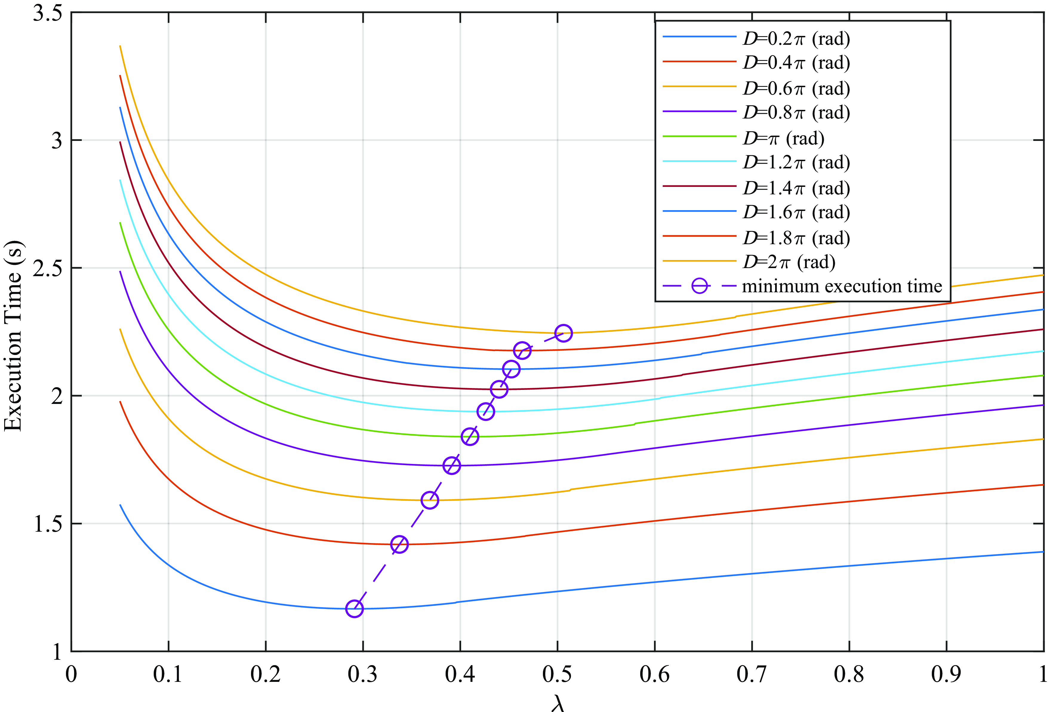
Figure 6.
Variation curve between the asymmetric parameter
![]() $\lambda$
and the execution time according to the displacement (V
m
=10 rad/s, A
m
=12 rad/s2, J
m
=40 rad/s3, S
dm
=150 rad/s4).
$\lambda$
and the execution time according to the displacement (V
m
=10 rad/s, A
m
=12 rad/s2, J
m
=40 rad/s3, S
dm
=150 rad/s4).
As shown in Fig. 6, when the displacement isn’t so large,
![]() $\lambda$
of achieving the minimum execution time is close to zero and increases gradually as the displacement is lengthened. But even though the displacement is very large, it might be impossible to achieve the minimum execution time for
$\lambda$
of achieving the minimum execution time is close to zero and increases gradually as the displacement is lengthened. But even though the displacement is very large, it might be impossible to achieve the minimum execution time for
![]() $\lambda$
= 1 due to the relationship between the kinematic constraints (velocity, acceleration and jerk). Fig. 7 shows the relationship between
$\lambda$
= 1 due to the relationship between the kinematic constraints (velocity, acceleration and jerk). Fig. 7 shows the relationship between
![]() $\lambda$
and the execution time according to the maximum snap of the deceleration stage when giving the kinematic constraints (displacement, velocity, acceleration and jerk). As illustrated in Fig. 7,
$\lambda$
and the execution time according to the maximum snap of the deceleration stage when giving the kinematic constraints (displacement, velocity, acceleration and jerk). As illustrated in Fig. 7,
![]() $\lambda$
achieving the minimum execution time is small as the maximum snap of the deceleration stage is decreased and inversely
$\lambda$
achieving the minimum execution time is small as the maximum snap of the deceleration stage is decreased and inversely
![]() $\lambda$
is approaching 1 as the snap is increased. If the maximum snap of the deceleration stage is larger than a certain value, the required
$\lambda$
is approaching 1 as the snap is increased. If the maximum snap of the deceleration stage is larger than a certain value, the required
![]() $\lambda$
is equal to 1.
$\lambda$
is equal to 1.

Figure 7.
Variation curve of the execution time versus the asymmetric parameter
![]() $\lambda$
according to the maximum snap of the deceleration stage (D =πrad, V
m
=10rad/s, A
m
=12 rad/s2, J
m
=40 rad/s3, S
dm
=150 rad/s4).
$\lambda$
according to the maximum snap of the deceleration stage (D =πrad, V
m
=10rad/s, A
m
=12 rad/s2, J
m
=40 rad/s3, S
dm
=150 rad/s4).
Hence, the minimum execution time is generated in the same model as the symmetric profile. But the large threshold of snap is not prerequisite, because the purpose of this article is to enhance the effectiveness of the motion more in the operation of attaching importance to the smoothness of the motion. As the kinematic indices (velocity, acceleration and jerk) reached their limits, the efficiency is more increased but the smoothness of the motion is more decreased, if the bounded value of snap is very large.
It is difficult to calculate the asymmetric parameter
![]() $\lambda$
analytically. This article presents an algorithm to get the asymmetric parameter
$\lambda$
analytically. This article presents an algorithm to get the asymmetric parameter
![]() $\lambda$
for achieving the minimum execution time under the kinematic constraints when restricting the maximum snap of the deceleration stage.
$\lambda$
for achieving the minimum execution time under the kinematic constraints when restricting the maximum snap of the deceleration stage.
Algorithm 1: Decision of
![]() $\lambda$
satisfying the minimum execution time
$\lambda$
satisfying the minimum execution time

Algorithm 2: Calculation procedure for time-scaled synchronized trajectory generation

As shown in Fig. 6, we decide the asymmetric parameter
![]() $\lambda$
according to the previously given displacement using the algorithm and may use the values effectively in the online control.
$\lambda$
according to the previously given displacement using the algorithm and may use the values effectively in the online control.
2.4. Synchronization of multi-axis motions
When
![]() $\lambda$
is given the certain value, the time-scaled synchronization and velocity synchronization method presented in ref. [Reference Fang, Hu, Liu, Shao, Qi and Peng8] can be applied to this trajectory planning method for synchronization of multi-axis motions. As above-mentioned, when limiting the maximum snap of the deceleration stage, not only the smoother profile is generated than the symmetric profile in the deceleration stage, but the motion time can be more decreased. Algorithm 2 presents the calculation procedure for generating a time-scaled synchronized trajectory using algorithm 1.
$\lambda$
is given the certain value, the time-scaled synchronization and velocity synchronization method presented in ref. [Reference Fang, Hu, Liu, Shao, Qi and Peng8] can be applied to this trajectory planning method for synchronization of multi-axis motions. As above-mentioned, when limiting the maximum snap of the deceleration stage, not only the smoother profile is generated than the symmetric profile in the deceleration stage, but the motion time can be more decreased. Algorithm 2 presents the calculation procedure for generating a time-scaled synchronized trajectory using algorithm 1.
3. Results and discussion
3.1. 3 DOF robotic manipulator: trajectory planning on a straight line motion of the end-effector in the task space
Firstly, we consider 3 DOF robotic manipulator as the typical case, where we generate a straight line motion of the end-effector in the task space. The coordinates and displacements of the initial and end points of the end-effector are given in Table I.
Table I. End-effector coordinates at the initial and end points and corresponding displacements.

The diagram of this robotic manipulator and rectilinear motion trajectory in the Cartesian coordinate are shown in Fig. 8.
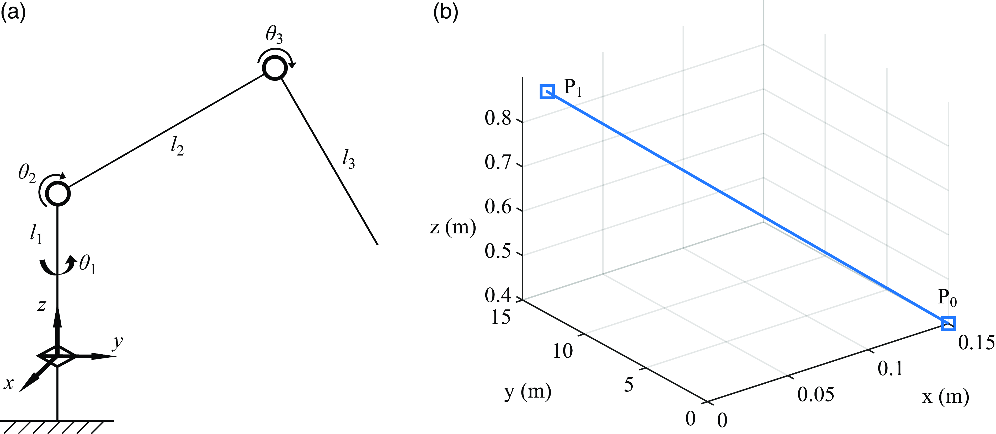
Figure 8. (a) Diagram of 3 DOF robotic manipulator; (b) rectilinear motion trajectory in the Cartesian coordinate (P 0-initial point, P 1-end point).
Xiao et al. and Fang et al. already performed the trajectory planning with the task data [Reference Fang, Hu, Liu, Shao, Qi and Peng8, Reference Xiao, Du and Dong10]. Based on this, we generate the trajectories with the constraints shown in Table II to illustrate the asymmetric S-curve trajectories under the different kinematic constraints. Then, for asymmetry, the jerks given in Table II are set to be the maximum allowable jerks in the acceleration stage and the maximum allowable jerks in the deceleration stage equal to the halves of jerks in the acceleration stage. The maximum allowable snap of the acceleration stage is set to be
![]() $275.22m/s^{4},125.10m/s^{4}$
and
$275.22m/s^{4},125.10m/s^{4}$
and
![]() $41.70m/s^{4}$
in the three constraint sets, respectively. Then, the allowable maximum snaps of the deceleration stage are obtained from Eq. (4) and Eq. (9) directly.
$41.70m/s^{4}$
in the three constraint sets, respectively. Then, the allowable maximum snaps of the deceleration stage are obtained from Eq. (4) and Eq. (9) directly.
Figs. 9-13 illustrate the trajectories of displacements, velocities, accelerations, jerks and snaps of the end-effector about every axis and angle position trajectories of every joint are shown in Fig. 14.
Since the displacement, velocity, acceleration and jerk trajectories of end-effector are continuous and zero at the initial moment and final moment of motion as illustrated in Figs. 9-14, the end-effector moves smoothly under the given constraints.
Therefore, impulses can be avoided and it is favourable to the exact control of the joints.
3.2. 6 DOF robotic manipulator: the synchronized trajectory planning in the joint space
We apply the proposed method to the trajectory planning of the 6 DOF robotic manipulator. Then, the trajectory is generated in the joint space. The simulation data is set to be identical to the data in refs. [Reference Fang, Hu, Liu, Shao, Qi and Peng8, Reference Perumaal and Jawahar30, Reference Chettibi, Lehtihet, Haddad and Hanchi39]. Table III shows the kinematic constraints and positions of joints.
Table II. Kinematic constraints of the robot along every axis in the task space.

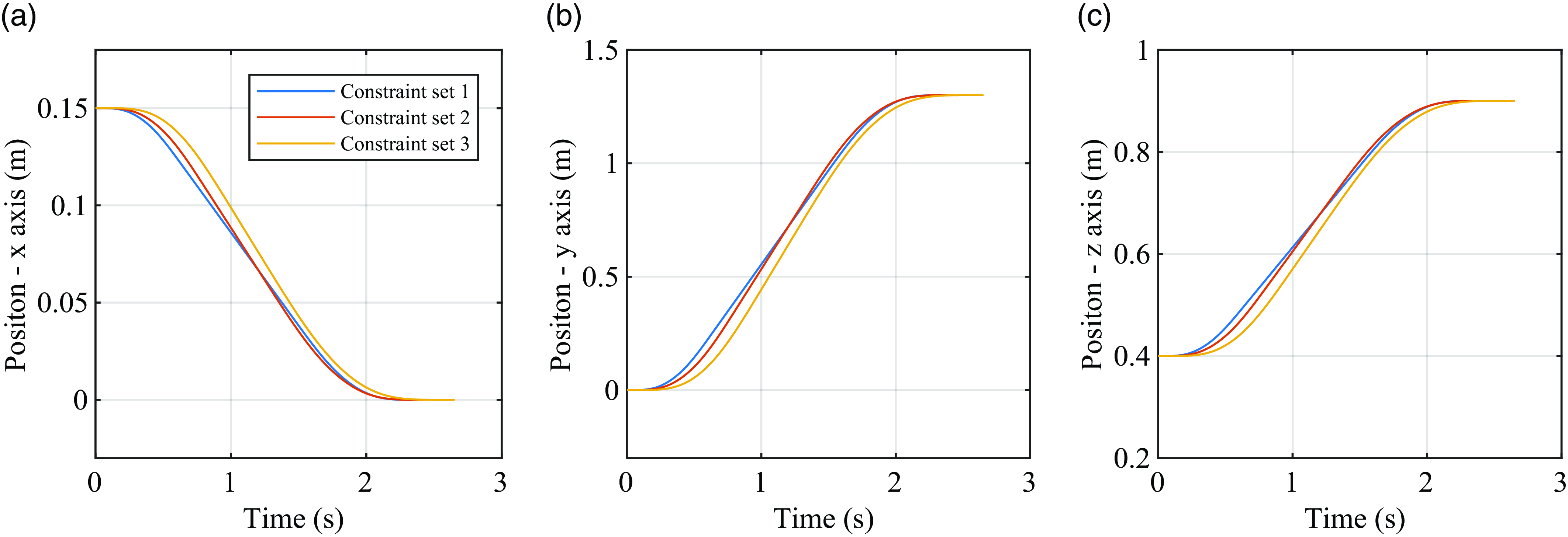
Figure 9. End-effector displacement trajectories about (a) x-axis; (b) y-axis; and (c) z-axis.
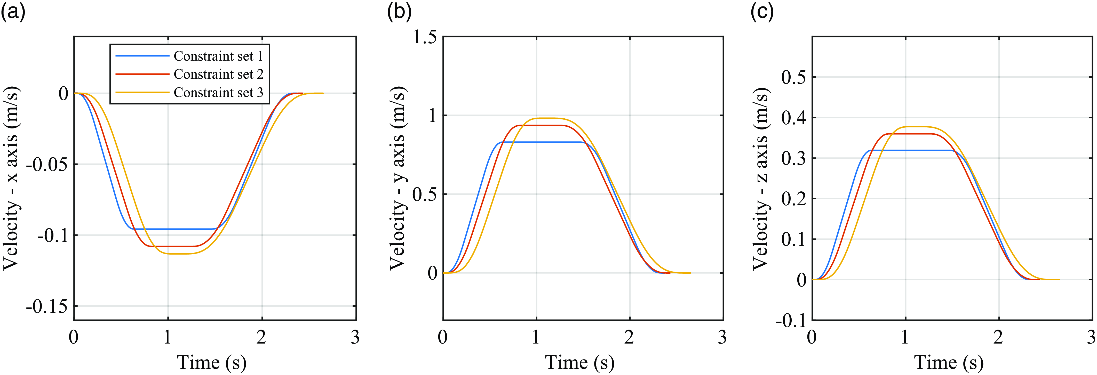
Figure 10. End-effector velocity trajectories about (a) x-axis; (b) y-axis; and (c) z-axis.

Figure 11. End-effector acceleration trajectories about (a) x-axis; (b) y-axis; and (c) z-axis.
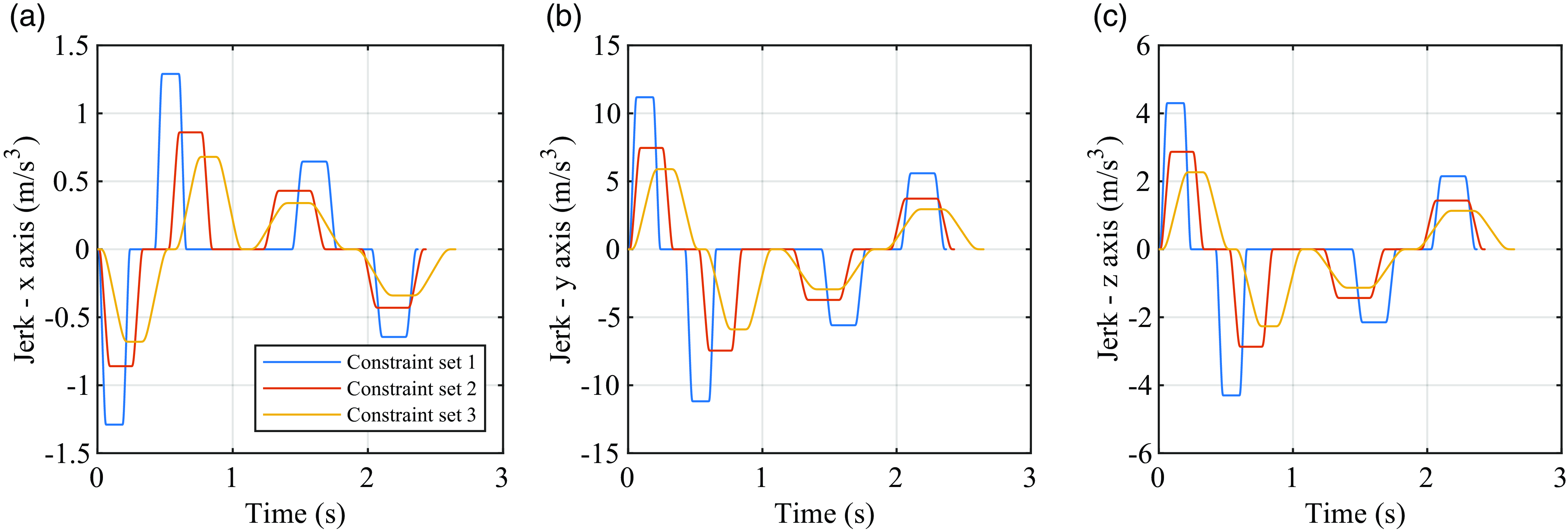
Figure 12. End-effector jerk trajectories about (a) x-axis; (b) y-axis; and (c) z-axis.
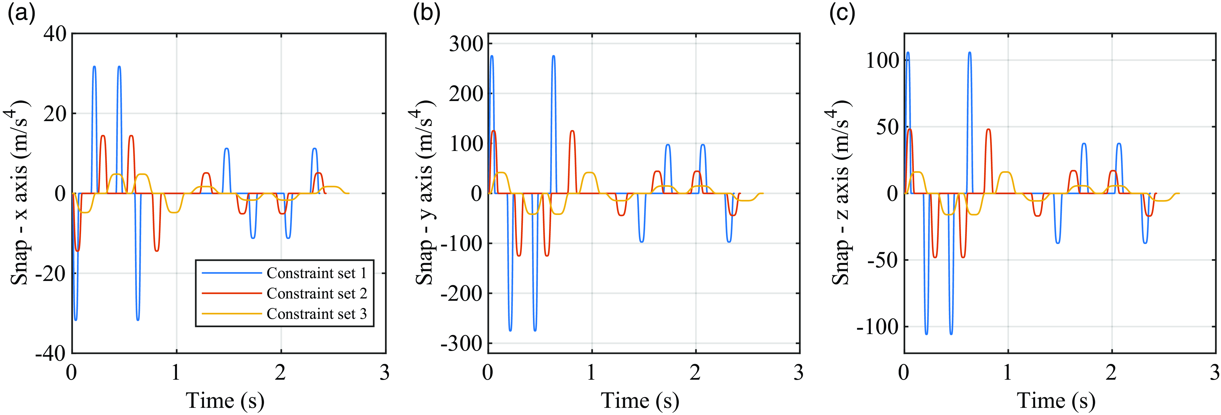
Figure 13. End-effector snap trajectories about (a) x-axis; (b) y-axis; and (c) z-axis.
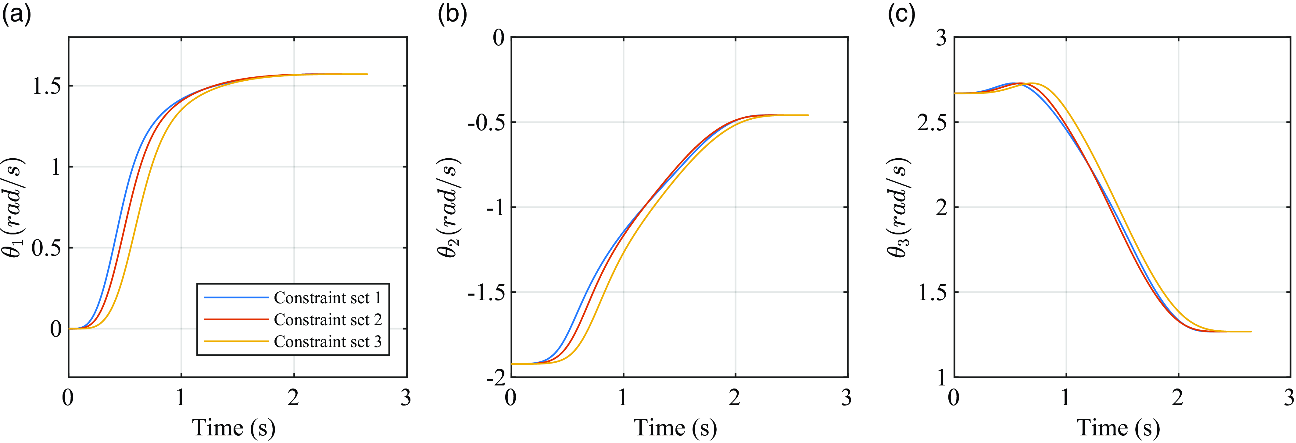
Figure 14. Angle position trajectories of (a) joint 1; (b) joint 2; and (c) joint 3.
The maximum allowable jerk in the acceleration stage is equal to the data given in Table III. Also, the snap constraints in the deceleration stage are set to be 150 rad/s4. Then, the snap constraints in the acceleration stage are determined by Eq. (9) and
![]() $\lambda$
obtained using the algorithm 1. Table IV shows the comparative results of the execution time with the real maximum jerk of joints in the unsynchronized case in ref. [Reference Fang, Hu, Liu, Shao, Qi and Peng8]. As can be shown in Table IV, the execution times of all joints are smaller and the real maximum jerks are shortened about 30% lower than that of the trajectories presented in ref. [Reference Fang, Hu, Liu, Shao, Qi and Peng8].
$\lambda$
obtained using the algorithm 1. Table IV shows the comparative results of the execution time with the real maximum jerk of joints in the unsynchronized case in ref. [Reference Fang, Hu, Liu, Shao, Qi and Peng8]. As can be shown in Table IV, the execution times of all joints are smaller and the real maximum jerks are shortened about 30% lower than that of the trajectories presented in ref. [Reference Fang, Hu, Liu, Shao, Qi and Peng8].
Table V illustrates the comparative results of the real maximum jerk and snap of joints in the time-scaled synchronized case with respect to that in ref. [Reference Fang, Hu, Liu, Shao, Qi and Peng8]. As shown in Table V, it can be seen that the real maximum jerk and snap of all joints in the deceleration stage are much smaller.
Fig. 15 shows the results given by the time-scaled synchronization method proposed in this paper.
Table III. Positions and kinematic constraints of the robot joints.

Table IV. Comparative results of the execution time and the jerk of joints in the unsynchronized case.

Table V. Comparative results of the jerk and snap of joints calculated by the time-scaled synchronization.

The position, velocity, acceleration and jerk of all the joints satisfy the kinematical constraints in Table III, and the trajectories are smooth and continuous during the whole motion. And Fig. 16 shows the end-effector trajectories of the UR5 robot manipulator (position, velocity, acceleration and jerk trajectories) in the task space when every joint is moved along the trajectories shown in Fig. 15.
As shown in Fig. 16, since the displacement, velocity, acceleration and jerk trajectories of end-effector are continuous and zero at the initial and final point of motion, the end-effector moves smoothly. Thus, it can be seen that the smooth starting and ending of trajectory could also be ensured.
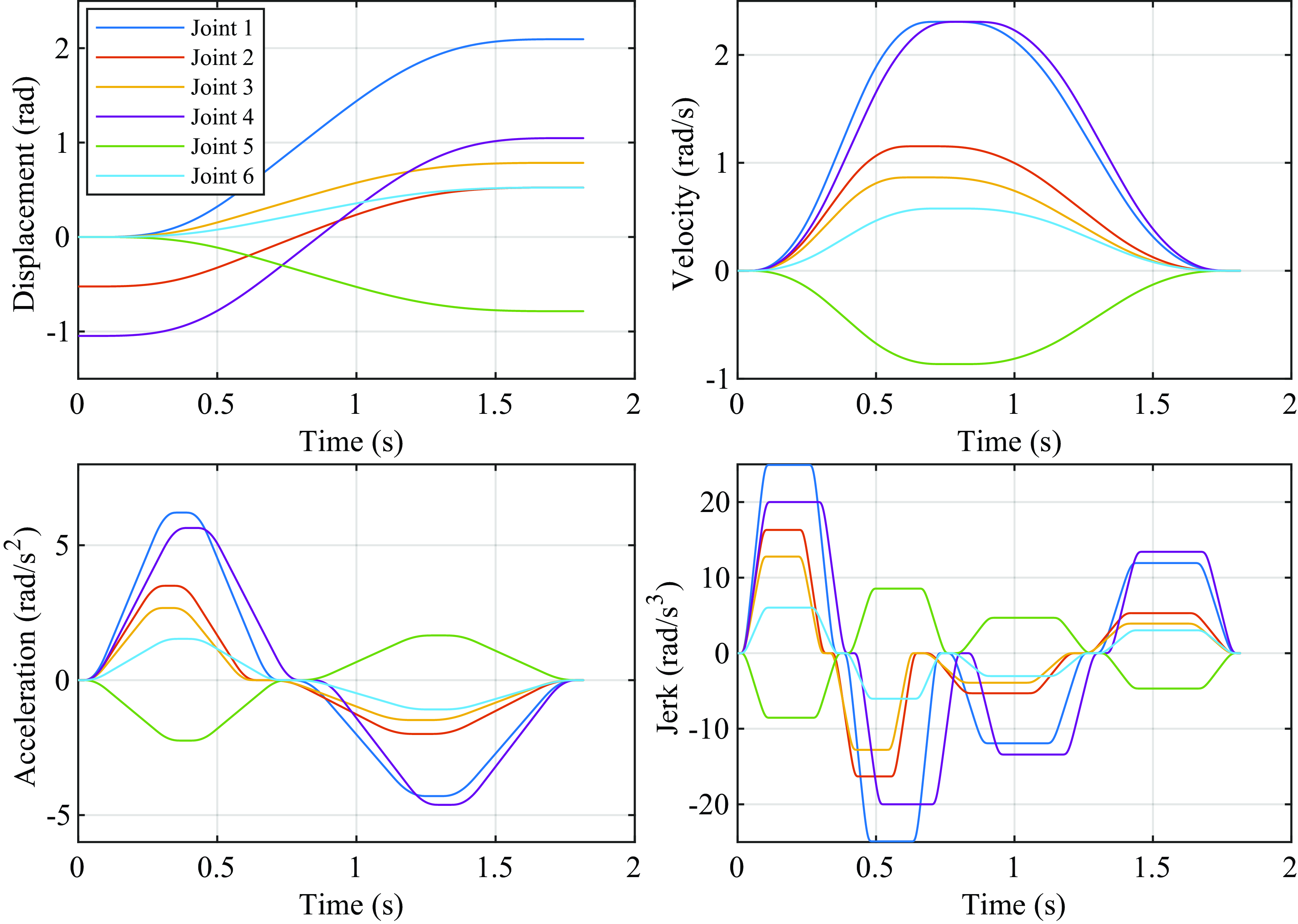
Figure 15. Asymmetric S-curve profiles generated by new time-scaled synchronization.
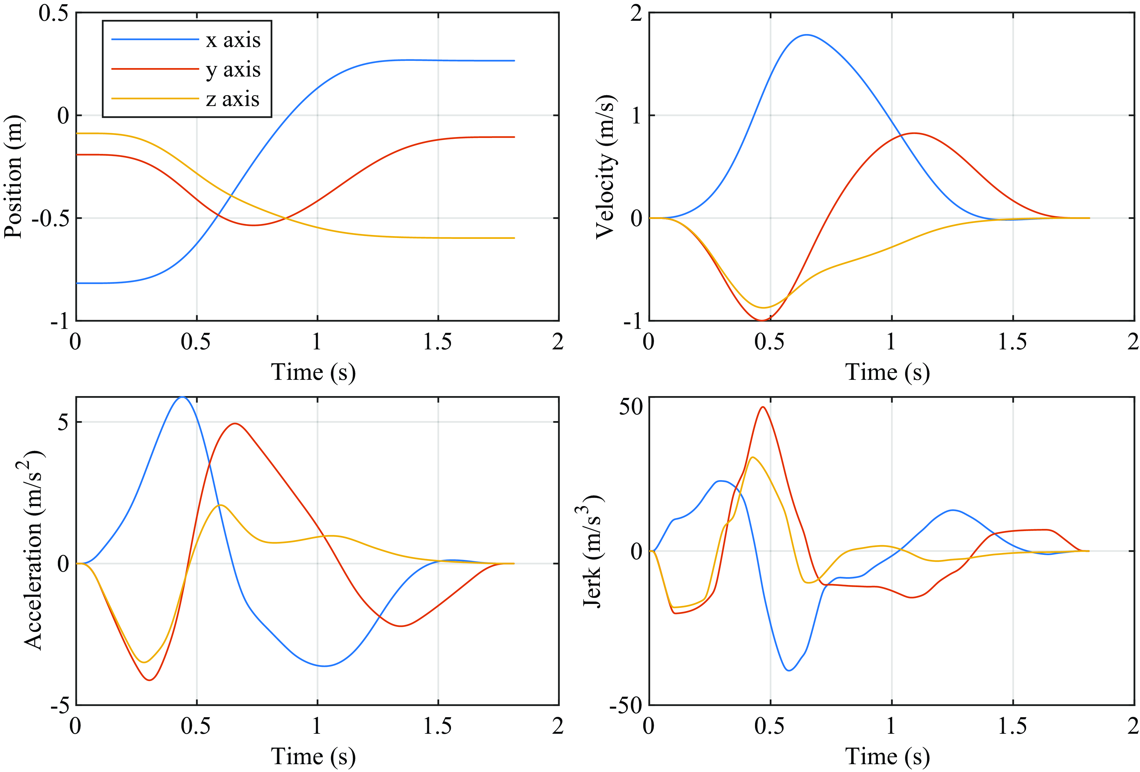
Figure 16. End-effector trajectories of the 6 DOF robot manipulator.
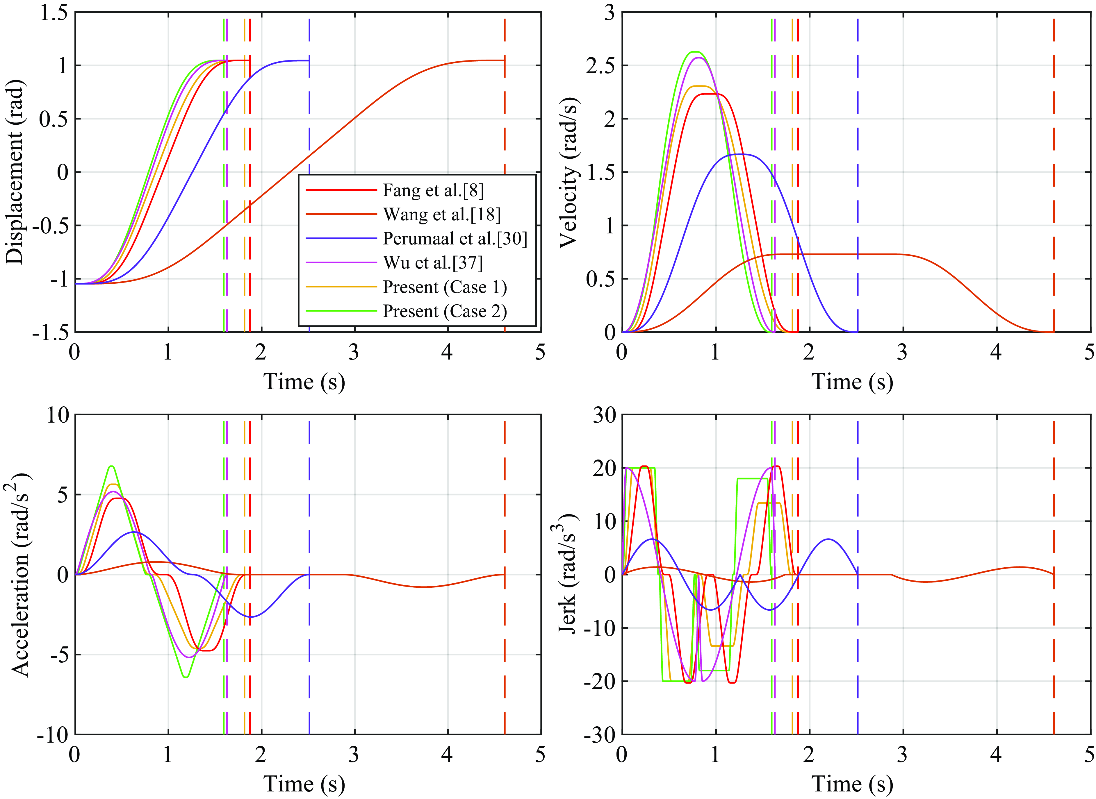
Figure 17. Motion profiles of joint 4 for different trajectory models.
Also, we analyse the execution time with four different types of trajectories [Reference Fang, Hu, Liu, Shao, Qi and Peng8, Reference Wang, Wang, Huang, Zhao and Quan18, Reference Perumaal and Jawahar30, Reference Wu, Chen, Bao, Wang, Zhang and Xu37] using the kinematical constraints in Table III. We perform the calculation of two cases for the proposed method, where the jerk given in Table III is set to be the allowable maximum jerks of the acceleration stage. For 1st calculation, the maximum snap of the deceleration stage is set to be
![]() $150rad/s^{4}$
and
$150rad/s^{4}$
and
![]() $\lambda$
is determined by using the algorithm 1 for every joint. For 2nd calculation, the maximum snap of the acceleration stage is set to be
$\lambda$
is determined by using the algorithm 1 for every joint. For 2nd calculation, the maximum snap of the acceleration stage is set to be
![]() $700rad/s^{4}$
and
$700rad/s^{4}$
and
![]() $\lambda$
is set to be 0.9 for all joints. Then, the maximum snaps of the deceleration or acceleration stage are obtained from Eq. (4) and Eq. (9). Fig. 17 shows the motion profiles of joint 4, which is generated by the benchmark methods and the proposed one. The motion profiles generated by [Reference Kornmaneesang and Chen15] show that the real maximum jerk has the lowest value compared with other algorithms, which resulted in the longest execution time. Table VI presents the measured performances including the execution time and real maximum jerk of acceleration and deceleration stage by the benchmark algorithms and the proposed one for the test task. The results show that the proposed method yielded the smaller execution time than the benchmark ones [Reference Fang, Hu, Liu, Shao, Qi and Peng8, Reference Wang, Wang, Huang, Zhao and Quan18, Reference Perumaal and Jawahar30]. Compared with [Reference Wu, Chen, Bao, Wang, Zhang and Xu37], the obtained execution time for 1st calculation is larger, but it is shorter for 2nd calculation. As shown in Table VI and Fig. 17, if the maximum snap is set as a large value relative to the jerk constraints, the jerks will reach the maximal value in a comparatively short period so that the shorter execution time is generated. However, the generated jerk profiles will lead to harmful vibrations. If adjusting the allowable maximum snap and jerk in the deceleration stage, it is possible to control the relationship between the execution time and smoothness.
$\lambda$
is set to be 0.9 for all joints. Then, the maximum snaps of the deceleration or acceleration stage are obtained from Eq. (4) and Eq. (9). Fig. 17 shows the motion profiles of joint 4, which is generated by the benchmark methods and the proposed one. The motion profiles generated by [Reference Kornmaneesang and Chen15] show that the real maximum jerk has the lowest value compared with other algorithms, which resulted in the longest execution time. Table VI presents the measured performances including the execution time and real maximum jerk of acceleration and deceleration stage by the benchmark algorithms and the proposed one for the test task. The results show that the proposed method yielded the smaller execution time than the benchmark ones [Reference Fang, Hu, Liu, Shao, Qi and Peng8, Reference Wang, Wang, Huang, Zhao and Quan18, Reference Perumaal and Jawahar30]. Compared with [Reference Wu, Chen, Bao, Wang, Zhang and Xu37], the obtained execution time for 1st calculation is larger, but it is shorter for 2nd calculation. As shown in Table VI and Fig. 17, if the maximum snap is set as a large value relative to the jerk constraints, the jerks will reach the maximal value in a comparatively short period so that the shorter execution time is generated. However, the generated jerk profiles will lead to harmful vibrations. If adjusting the allowable maximum snap and jerk in the deceleration stage, it is possible to control the relationship between the execution time and smoothness.
3.3. Estimation of residual vibration
To assess the efficiency of the proposed method, we have carried out the analysis of residual vibration.
The dynamic model of a simplified single-axis motion stage is shown in Fig. 18. It includes a flexible base structure with a weight of
![]() $m_{1}$
, holding a motor to move a mass with an equivalent weight of
$m_{1}$
, holding a motor to move a mass with an equivalent weight of
![]() $m_{2}$
. The friction force between the moving mass and the machine base is ignored. The dynamics of the flexible base is assumed to be a single-degree-of-freedom mass-spring-damper system, with a spring stiffness
$m_{2}$
. The friction force between the moving mass and the machine base is ignored. The dynamics of the flexible base is assumed to be a single-degree-of-freedom mass-spring-damper system, with a spring stiffness
![]() $k$
and damping coefficient
$k$
and damping coefficient
![]() $c$
.
$c$
.
Table VI. Comparative results of several planning methods.
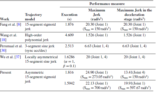
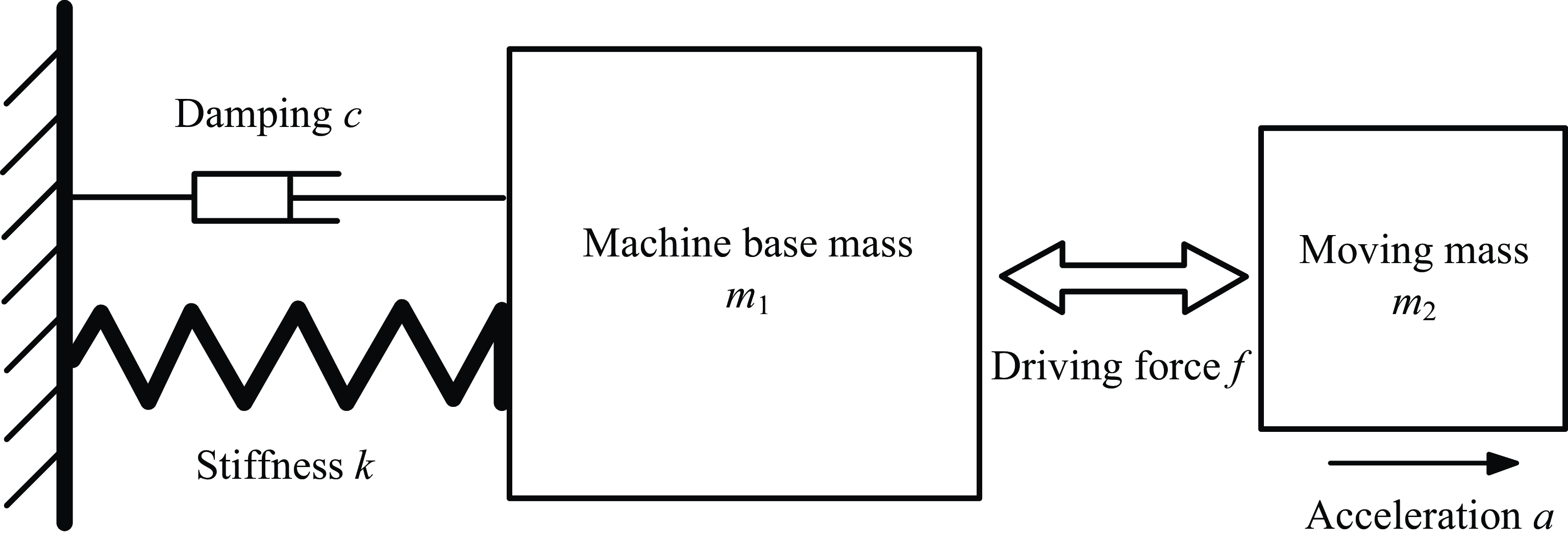
Figure 18. A single-degree-of-freedom mass-spring-damper system.
Where the moving mass
![]() $m_{2}$
is driven with an acceleration
$m_{2}$
is driven with an acceleration
![]() $a$
, the reaction force on the base structure
$a$
, the reaction force on the base structure
![]() $m_{1}$
will be
$m_{1}$
will be
![]() $F=m_{2}a$
.
$F=m_{2}a$
.
The dynamics of the base structure can be expressed as
Or
where
![]() $\omega _{n}$
is the angular natural frequency of the base structure,
$\omega _{n}$
is the angular natural frequency of the base structure,
![]() $\xi$
is the damping ratio, and
$\xi$
is the damping ratio, and
![]() $x$
is the vibration response of the base structure.
$x$
is the vibration response of the base structure.
To carry out the simulation study, it is assumed that the ratio of the moving mass over the machine base is 0.1, the undamped natural frequency of the base is 24 Hz, with a damping ratio of 3%, that is,
![]() $m_{2}/m_{1}=0.1,\omega _{n}=150.8rad/s$
(i.e.,
$m_{2}/m_{1}=0.1,\omega _{n}=150.8rad/s$
(i.e.,
![]() $f_{n}$
= 24 Hz) and
$f_{n}$
= 24 Hz) and
![]() $\xi =3\%$
[Reference Li35].
$\xi =3\%$
[Reference Li35].
For comparison, three different motion profiles are evaluated, including the locally asymmetrical profile, symmetric sigmoid S-curve profile and the proposed asymmetric sigmoid S-curve profile. The residual vibration of the base frame is then determined by considering the Eq. (35) to obtain the stage vibration. The kinematic constraints are shown in Table VII and were used in ref. [Reference Li35].
Table VII. Displacement and kinematic constraints.

We set
![]() $\alpha =1,\beta =0.265$
for the locally asymmetrical 15-segment sine jerk profile [Reference Wu, Chen, Bao, Wang, Zhang and Xu37] and the maximum snap is set to be
$\alpha =1,\beta =0.265$
for the locally asymmetrical 15-segment sine jerk profile [Reference Wu, Chen, Bao, Wang, Zhang and Xu37] and the maximum snap is set to be
![]() $5000m/s^{4}$
for the symmetric 15-segment sigmoid jerk profile [Reference Fang, Hu, Liu, Shao, Qi and Peng8]. We make an analysis of two cases for the proposed method, where the jerk given in Table VII is set to be the maximum allowable jerks of the acceleration stage and the maximum allowable jerks of the deceleration stage are set to be
$5000m/s^{4}$
for the symmetric 15-segment sigmoid jerk profile [Reference Fang, Hu, Liu, Shao, Qi and Peng8]. We make an analysis of two cases for the proposed method, where the jerk given in Table VII is set to be the maximum allowable jerks of the acceleration stage and the maximum allowable jerks of the deceleration stage are set to be
![]() $70m/s^{3}$
and
$70m/s^{3}$
and
![]() $30m/s^{3}$
, respectively. The maximum snaps of the acceleration stage are set to be
$30m/s^{3}$
, respectively. The maximum snaps of the acceleration stage are set to be
![]() $8000m/s^{4}$
and
$8000m/s^{4}$
and
![]() $5000m/s^{4}$
. Then, the maximum snaps of the deceleration stage are obtained from Eq. (4) and Eq. (9) directly. The simulated motion profiles of the moving mass are shown in Fig. 19, and the vibrations of the base structure excited by the stage motion using the four profiles are shown in Fig. 20. As shown in Fig. 19, the total execution time for the three profiles (i.e., [Reference Fang, Hu, Liu, Shao, Qi and Peng8], [Reference Wu, Chen, Bao, Wang, Zhang and Xu37] and the present method (case 1)) are all same as 0.9545s. And the execution time for the present method (case 2) is 1.0525s. Then, it is clear that the residual vibration excited by the locally asymmetrical sine jerk profile is the worst, with a peak-to-peak value of about 3
$5000m/s^{4}$
. Then, the maximum snaps of the deceleration stage are obtained from Eq. (4) and Eq. (9) directly. The simulated motion profiles of the moving mass are shown in Fig. 19, and the vibrations of the base structure excited by the stage motion using the four profiles are shown in Fig. 20. As shown in Fig. 19, the total execution time for the three profiles (i.e., [Reference Fang, Hu, Liu, Shao, Qi and Peng8], [Reference Wu, Chen, Bao, Wang, Zhang and Xu37] and the present method (case 1)) are all same as 0.9545s. And the execution time for the present method (case 2) is 1.0525s. Then, it is clear that the residual vibration excited by the locally asymmetrical sine jerk profile is the worst, with a peak-to-peak value of about 3
![]() $\mu m$
. For the symmetric sigmoid jerk profile, the residual vibration has a peak-to-peak value of about 2.2
$\mu m$
. For the symmetric sigmoid jerk profile, the residual vibration has a peak-to-peak value of about 2.2
![]() $\mu m$
, which is about 1.4 times better than the locally asymmetric profile. As shown in Fig. 20, the proposed method shows the best performance with a minimized vibration, where the residual vibration has a peak-to-peak value of about 1.9
$\mu m$
, which is about 1.4 times better than the locally asymmetric profile. As shown in Fig. 20, the proposed method shows the best performance with a minimized vibration, where the residual vibration has a peak-to-peak value of about 1.9
![]() $\mu m$
for case 1 and about 0.25
$\mu m$
for case 1 and about 0.25
![]() $\mu m$
for case 2.
$\mu m$
for case 2.
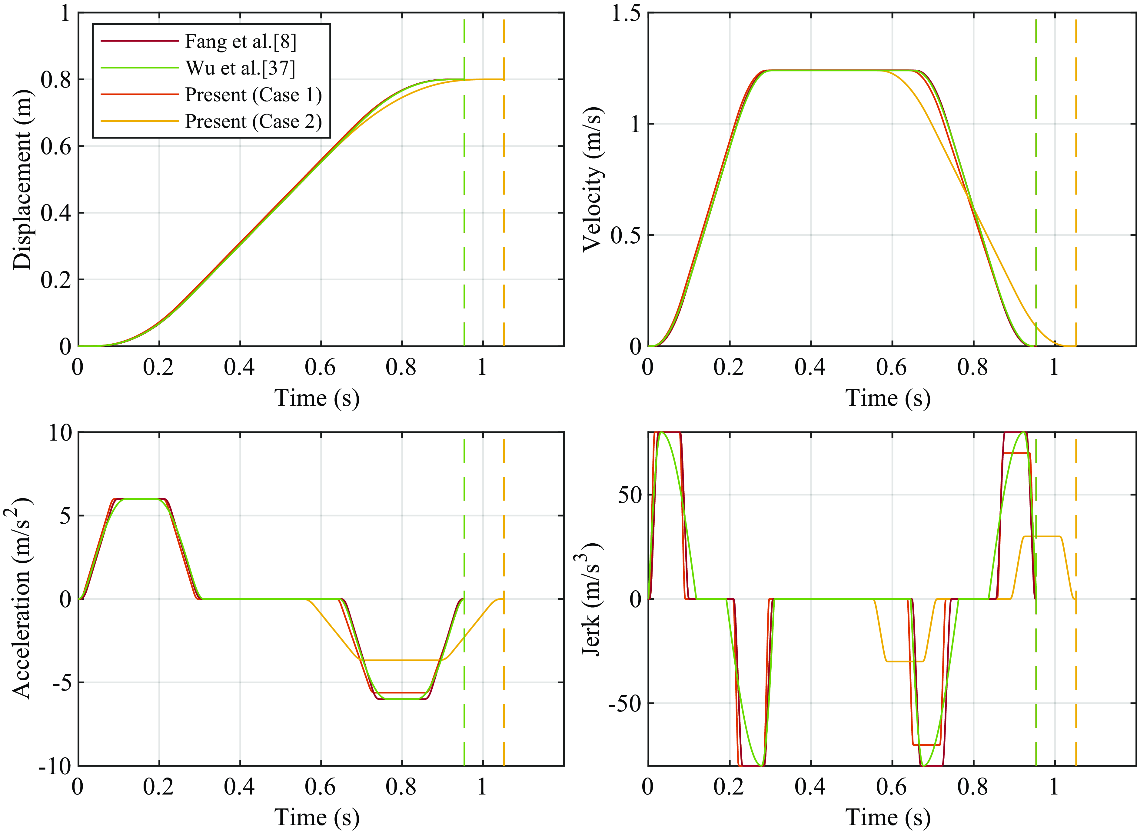
Figure 19. Motion profiles for different trajectory models.

Figure 20. Vibration response for different trajectory models.
As seen in the results obtained by [Reference Fang, Hu, Liu, Shao, Qi and Peng8] and the present (case 2), when the maximum snap of the acceleration stage is specified, the execution time is more lengthened than one of the symmetric profiles, but the generating profile is smoother and the residual vibration is smaller than one of the symmetric profiles.
The results show clearly that the performance of reducing vibrations on the machinery is good and demonstrate an important characteristic of the proposed profile suitable for high-speed point-to-point motion. The proposed asymmetric sigmoid profile is generated by adding one asymmetric parameter in the symmetric one presented in ref. [Reference Fang, Hu, Liu, Shao, Qi and Peng8], and thus, the calculation quality and time to get the optimal solution is less different for two methods. In (Fang et al. [Reference Fang, Hu, Liu, Shao, Qi and Peng8]), the experiments were conducted on a 6 DOF manipulator Universal Robots UR5 and the practical usability of the proposed approach was validated. The proposed method can be implemented in the same way as presented in ref. [Reference Fang, Hu, Liu, Shao, Qi and Peng8].
4. Conclusion
In this paper, a new method of planning asymmetric S-curve trajectories based on an expanded jerk profile is presented for smoothness and time optimality. The improved piecewise sigmoid jerk profile has been generated by introducing an asymmetric parameter. All the trajectories generated are continuous and infinitely differentiable. In addition, the values of the two end points of all derivatives are always zero. When the maximum snap of the acceleration stage is specified, the execution time is more lengthened than one of the symmetric profiles, but the generating profile is smoother and the residual vibration is smaller than one of the symmetric. However, when the maximum snap of the deceleration stage is specified, not only the smoother profile is generated but also the execution time is shorter than one of the symmetric. Thus, in the operation of assigning the smoothness of the motion, both smoothness and efficiency can be more raised. The minimum execution time has been achieved under the kinematic constraints in terms of the analytical algorithm. The results obtained through several benchmark experiments show that the proposed method can be used as the effective tool for the smooth trajectory planning of the industrial robots.
Future work will be devoted to applying the proposed method for more delicate applications requiring a complex spatial path comprising multi-points.
Author contributions
CH, KS and UR conceived, designed the study, performed simulations and wrote the article.
Financial support
This research received no specific grant from any funding agency, commercial or not-for-profit sectors.
Competing interests
The authors declare none.
Ethical consideration
The authors declare none.


