Physical significance of artificial numerical noise in direct numerical simulation of turbulence

Abstract

Using clean numerical simulation (CNS) in which artificial numerical noise is negligible over a finite, sufficiently long interval of time, we provide evidence, for the first time, that artificial numerical noise in direct numerical simulation (DNS) of turbulence is approximately equivalent to thermal fluctuation and/or stochastic environmental noise. This confers physical significance on the artificial numerical noise of DNS of the Navier–Stokes equations. As a result, DNS on a fine mesh should correspond to turbulence under small internal/external physical disturbance, whereas DNS on a sparse mesh corresponds to turbulent flow under large physical disturbance. The key point is that all of them have physical meanings and so are correct in terms of their deterministic physics, even if their statistics are quite different. This is illustrated herein. Our paper provides a positive viewpoint regarding the presence of artificial numerical noise in DNS.

1. Introduction

Turbulence is one of the most challenging problems in fluid mechanics. It is widely accepted by the turbulence community that turbulent flows can be well described by the Navier–Stokes (NS) equations, which are related to the fourth millennium problem (Clay Mathematics Institute of Cambridge 2000). Direct numerical simulation (DNS) (Orszag 1970), which numerically solves the NS equations without any turbulent models, proved to be a milestone in fluid mechanics because it opened the era of numerical experiments (She, Jackson & Orszag 1991; Moin & Mahesh 1998; Scardovelli & Zaleski 1999; Gary & Richard 2010). However, artificial numerical noise caused by truncation and round-off errors is unavoidable for all numerical algorithms, including DNS. It was believed that tiny artificial numerical noise in DNS would not grow to reach large scale because of fluid viscosity. However, some scientists pointed out that turbulence governed by NS equations should be chaotic (Deissler 1986; Aurell et al. 1996; Berera & Ho 2018), and thus there exists the initial exponential growth of average error/uncertainty energy for two-dimensional (2-D) and three-dimensional (3-D) NS turbulence (Boffetta & Musacchio 2001, 2017; Ge, Rolland & Vassilicos 2023). Notably, Qin & Liao (2022) demonstrated that artificial numerical noise can lead to huge deviations in the DNS of 2-D turbulent Rayleigh–Bénard convection not only in spatio–temporal trajectory but also in statistics by considering the much more accurate results given by clean numerical simulation (CNS) (Liao 2009; Hu & Liao 2020; Liao 2023). Unlike DNS that uses double precision in general, CNS adopts multiple precision (Oyanarte 1990) with sufficient significant digits to greatly decrease the round-off error, as well as sufficiently high-order Taylor expansion (in time dimension) and small enough spacing for the pseudo-spectral method (in space dimension) to greatly decrease the truncation errors in time and space, respectively, so that the artificial numerical noise can be limited to a prescribed small level. As a result, artificial numerical noise in CNS can be negligible over a finite but long enough time interval suitable for calculating statistics. Hence, the CNS results lie close to the true solution of the turbulent flow under consideration and can be used as benchmark data. Therefore, one can carry out clean numerical experiments for turbulence using CNS, where the word ‘clean’ implies that the artificial numerical noise is much smaller than the true solution in a finite, prescribed long time interval $[0,T_{c}]$ , and thus can be neglected. Note that the artificial numerical noise might reach a macro level once the prescribed time $T_{c}$ has been exceeded, thereafter results given by CNS are also badly polluted by artificial numerical noise: the reason why, unlike DNS, simulation of CNS is stopped at a finite prescribed time $T_c$ . This is an obvious difference between DNS and CNS. In fact, from the viewpoint of CNS, a traditional DNS result using double precision often has a very small value of $T_c$ so that DNS is only a special case of CNS although unfortunately such a small $T_c$ is useless for calculating statistics.

To confirm the previously mentioned findings of Qin & Liao (2022) concerning 2-D turbulent Rayleigh–Bénard convection, Qin et al. (2024) recently used CNS to model a 2-D Kolmogorov turbulent flow subject to a periodic boundary condition and a periodic initial condition with a kind of spatial symmetry. In mathematics, it is obvious that the true solution of the corresponding 2-D Kolmogorov turbulent flow should have the same spatial symmetry for all $t \gt 0$ as the initial condition. It was found that the corresponding CNS result indeed maintains the same spatial symmetry as the initial condition throughout the whole time interval of simulation, clearly indicating that its numerical noise is indeed negligible so that it is indeed a clean simulation. However, the DNS result maintains the same spatial symmetry only at the beginning but quickly loses spatial symmetry completely: this clearly indicates that the small-scale artificial numerical noise of DNS, which is random and without spatial symmetry, indeed quickly grows to become large scale.

Recently, using CNS to solve a kind of 2-D turbulent Kolmogorov flow subject to a specially chosen initial condition that contains micro-level disturbances at different orders of magnitude, say, $O (10^{-20} )$ and $O (10^{-40} )$ , Liao & Qin (2025) discovered an interesting phenomenon, which they called ‘the noise-expansion cascade’ whereby all micro-level disturbances at different orders of magnitude evolute and grow continuously, step by step, as an inverse cascade, to reach the macro level. It was found that each disturbance could greatly change the characteristics of the 2-D turbulent Kolmogorov flow. This clearly indicates that each disturbance must be considered in the NS equations, even if the disturbance is many orders of magnitude smaller than others.

Note that, just like artificial numerical noise, both internal thermal fluctuation and external environmental noise are unavoidable in practice. The following fundamental questions arise about the relationships between artificial numerical noise and thermal fluctuations and/or environmental noise:

1. (i) Is artificial numerical noise in DNS approximately equivalent to thermal fluctuation and/or stochastic environmental noise?

2. (ii) What is the physical significance of artificial numerical noise in DNS?

3. (iii) Are there some turbulent flows whose statistics are sensitive to artificial numerical noise?

To the best of our knowledge, these are presently open questions. In this paper, we will answer them by first using CNS to carry out the clean numerical experiment for a 2-D turbulent Kolmogorov flow, and then comparing the CNS benchmark solution, whose artificial numerical noise is negligible, with DNS predictions where artificial numerical noise quickly grows to the macro level.

2. Mathematical model and numerical algorithm

Since DNS is mostly used to solve NS equations, let us consider here an incompressible flow in a 2-D square domain $[0, L]^2$ , called Kolmogorov flow (Arnold & Meshalkin 1960; Obukhov 1983) with the ‘Kolmogorov forcing’ that is stationary, monochromatic and sinusoidally varying in space with forcing scale $n_K$ and amplitude $\chi$ . Using the length scale $L/2\pi$ and the time scale $\sqrt {L/(2 \pi \xi)}$ , the corresponding non-dimensional NS equations in the form of streamfunction $\psi$ read (Chandler & Kerswell 2013)

(2.1) \begin{align} & \frac {\partial }{\partial t}\nabla ^{2}\psi +\frac {\partial (\psi, \nabla ^{2}\psi )}{\partial (x,y)}-\frac {1}{Re}\nabla ^{4}\psi +n_K\cos (n_Ky)=0, \end{align}

where $t$ denotes the time, $x$ and $y$ are the Cartesian coordinates within $x,y\in [0,2\pi ]$ , $\nabla ^{4}=\nabla ^{2}\nabla ^{2}$ where $\nabla ^{2}$ is the Laplace operator,

(2.2) \begin{align} \frac {\partial (a,b)}{\partial (x,y)}=\frac {\partial a}{\partial x}\frac {\partial b}{\partial y}-\frac {\partial b}{\partial x}\frac {\partial a}{\partial y} \end{align}

is the Jacobi operator, and $Re= ({\sqrt {\chi }}/{\nu }) ( {L}/{2\pi } )^{{3}/{2}}$ is the Reynolds number, in which $\nu$ denotes the fluid kinematic viscosity. We use here the periodic boundary condition

(2.3) \begin{align} & \psi (x,y,t)=\psi (x+2\pi, y,t)=\psi (x,y+2\pi, t), \end{align}

the initial condition

(2.4) \begin{align} & \psi (x,y,0)=-\tfrac{1}{2}[\cos (x+y)+\cos (x-y)], \end{align}

and the physical parameters $n_K=16$ and $Re=2000$ . All of these are exactly the same as those used by Liao & Qin (2025).

Since DNS is mostly used to solve NS equations, let us consider here a simple model about the influence of thermal fluctuation and/or stochastic environmental noise on turbulence in the frame of NS equations. According to the theory of statistical physics concerning thermal fluctuation (Landau & Lifshitz 1959), the mean square of velocity fluctuation is given by

(2.5) \begin{align} & \left\langle u_{th}^2 \right\rangle = \frac {k_B\langle T \rangle }{V\langle \rho \rangle }, \end{align}

where the subscript ‘th’ stands for thermal fluctuation, $k_B$ is the Boltzmann constant, $\langle T \rangle$ and $\langle \rho \rangle$ are the mean temperature and mass density. In this paper, the fluid is water at room temperature (20 $^{\circ }$ C), thus $k_B=1.38\times 10^{-23}$ J K $^{- 3}$ , $\langle T \rangle = 293.15$ K, and $\langle \rho \rangle = 998$ kg m $^{- 3}$ . Besides, $V$ is regarded as a unit volume. For simplicity, the tiny velocity fluctuation $u_{th}$ is regarded here as a kind of Gaussian white noise with standard deviation $\sigma =10^{-10}$ . For the 2-D turbulent flow, we have

(2.6) \begin{equation} u=-\frac {\partial \psi }{\partial y}, \;\;\; v = \frac {\partial \psi }{\partial x}, \end{equation}

where the streamfunction $\psi$ is governed by (2.1) to (2.4). Therefore, considering the additional velocity fluctuation $u_{th}$ governed by (2.5), the streamfunction $\psi ^*$ with thermal fluctuation term is given by

(2.7) \begin{equation} \psi ^*(x,y,t) = \int _0^y -(u+u_{th})\,{\rm d}y = \psi (x,y,t) - \int _0^y u_{th}(x,y,t)\,{\rm d}y. \end{equation}

Here the term $\int _0^y u_{th}\,{\rm d}y$ is calculated by the Itô stochastic integral (Pavliotis 2014). Note that the velocity fluctuation in the $y$ direction, i.e. $v_{th}$ , is given by $-\partial (\int _0^y u_{th}(x,y,t)\,{\rm d}y)/\partial x$ . Then $\psi ^*(x,y,t)$ is submitted in the governing equation (2.1) to calculate $\psi (x,y,t+\Delta t)$ that is further used to gain $\psi ^*(x,y,t+\Delta t)$ by (2.7), and so on. Note that one can also regard the term $ - \int _0^y u_{th}(x,y,t)\,{\rm d}y$ as stochastic environmental noise. In this way, both the thermal fluctuation of velocity field and/or stochastic environmental noise could have influence on the turbulent flow due to the chaotic property of turbulence. Note that the law of mass conservation is always satisfied under the thermal fluctuation of velocity field and/or stochastic environmental noise, since the streamfunction is used here.

On the one hand, we solve (2.1) to (2.4) plus random thermal fluctuation and/or stochastic environmental noise via (2.7) throughout the whole interval of time $t \in [0, 300]$ by means of CNS, whose artificial numerical noise is negligible. Here the CNS algorithm is based on the pseudo-spectral method with uniform mesh $1024 \times 1024$ in space, the 140th-order Taylor expansion (i.e. $M=140$ ) with time step $\Delta t=10^{-3}$ for temporal evolution, and especially 260 significant digits in multiple precision (i.e. $N_s = 260$ ) for all variables and parameters. The results are given the name CNS $^*$ , where $^*$ denotes that the CNS result is modified by (2.7) for thermal fluctuation and/or stochastic environmental noise whose evolution is governed by the NS equations (2.1) to (2.4). The corresponding CNS algorithm is exactly the same as that described by Liao & Qin (2025), and thus is neglected here.

On the other hand, we solve the same equations (2.1) to (2.4) without thermal fluctuation and/or stochastic environmental noise by means of DNS over the same interval of time $t \in [0, 300]$ , during which the artificial numerical noise quickly enlarges to macro level. Here we adopt DNS using the pseudo-spectral method with the same uniform mesh $1024 \times 1024$ in space, but the 4th-order Runge–Kutta method with time step $\Delta t=10^{-4}$ in temporal evolution, and double precision (i.e. $N_s = 16$ ) for all variables and parameters, whose results are titled DNS in this paper. As illustrated by Liao & Qin (2025), the artificial numerical noise of DNS quickly enlarges to the same order of magnitude as the true solution, in other words, its spatial–temporal trajectory rapidly becomes badly polluted by artificial numerical noise.

The relationships between artificial numerical noise in DNS and thermal fluctuation and/or environmental noise can be investigated in detail by comparing the CNS $^{*}$ result, whose artificial numerical noise is negligible throughout the whole interval of time $t\in [0,300]$ , with the DNS result, whose artificial numerical noise rapidly enlarges to the macro level. Our detailed findings are given as follows.

3. Physical essence of artificial numerical noise of DNS

3.1. Is numerical noise equivalent to thermal fluctuation and/or environmental noise?

Here, using the previously mentioned 2-D turbulent Kolmogorov flow as an example and by means of CNS plus the tiny modification (2.7) at each time step, we provide evidence that artificial numerical noise of DNS is approximately equivalent to thermal fluctuation and/or stochastic environmental noise.

First of all, it should be emphasised that, if thermal fluctuation is not considered, the CNS result retains the spatial symmetry in the whole time interval $t\in [0,300]$ , indicating that the numerical noise of the CNS result is indeed negligible throughout the whole time interval so that it is indeed clean, as described by Liao & Qin (2025). By contrast, the DNS result quickly loses this spatial symmetry, clearly indicating that it is badly polluted quickly by numerical noise (Liao & Qin 2025). Based on this known fact, we are quite sure that the CNS result (mentioned later) with thermal fluctuation is also clean and reliable in the whole time interval $t\in [0,300]$ .

Figure 1. Time histories of the spatially averaged (a) kinetic energy dissipation rate $\langle D\rangle _A$ and (b) enstrophy dissipation rate $\langle D_{\Omega }\rangle _A$ of the 2-D turbulent Kolmogorov flow: CNS $^*$ (red solid line) and DNS (blue dashed line).

However, when considering thermal fluctuation and/or stochastic environmental noise via (2.7) at each time step, the time histories of the spatially averaged kinetic energy dissipation rate $\langle D\rangle _A$ as well as enstrophy dissipation rate $\langle D_{\Omega }\rangle _A$ given by CNS $^*$ and DNS are almost the same, especially for $t \gt 100$ which corresponds to a relatively stable state of turbulence, as shown in figure 1. Note that the definitions of the statistics as well as the statistic operators used in this paper are described in the supplementary material available at http://doi.org/10.1017/jfm.2025.200. Figure 2 shows that the probability density functions (PDFs) of the kinetic energy dissipation rate $D(x,y,t)$ and the kinetic energy $E(x,y,t)$ given by CNS $^{*}$ and DNS agree quite well, when the integration interval of time is $t \in [100, 300]$ corresponding to a relatively stable state of turbulence (as illustrated in figure 1). Similarly, the PDFs of the enstrophy dissipation rate $D_\Omega (x,y,t)$ and the enstrophy $\Omega (x,y,t)$ given by CNS $^{*}$ and DNS also agree quite well, as shown in figure 3. Furthermore, figure 4 illustrates that the temporal averaged kinetic energy spectra $\langle E_k \rangle _{t}$ and the spatio–temporal-averaged scale-to-scale energy fluxes $\langle \Pi ^{[l]} \rangle$ of the 2-D turbulent Kolmogorov flow given by CNS $^*$ and DNS are also in accord with each other. In addition, as shown in figure 4, both the CNS $^*$ and the DNS results give the Kolmogorov $-5/3$ power law of $\langle E_k \rangle _{t}$ when $k\lt n_K$ , as well as the inverse energy cascade (Boffetta & Ecke 2012; Alexakis & Biferale 2018). In addition, figure 5 shows that the spatio–temporal-averaged scale-to-scale enstrophy fluxes $\langle \Pi _\Omega ^{[l]} \rangle$ given by CNS $^*$ and DNS also agree quite well, where the direct enstrophy cascade (Boffetta & Ecke 2012; Alexakis & Biferale 2018) exists.

Figure 2. The PDFs of (a) the kinetic energy dissipation rate $D(x,y,t)$ and (b) the kinetic energy $E(x,y,t)$ of the 2-D turbulent Kolmogorov flow, where the integration is taken in $(x,y)\in [0,2\pi )^2$ and $t \in [100, 300]$ : CNS $^*$ (red line) and DNS (blue circles).

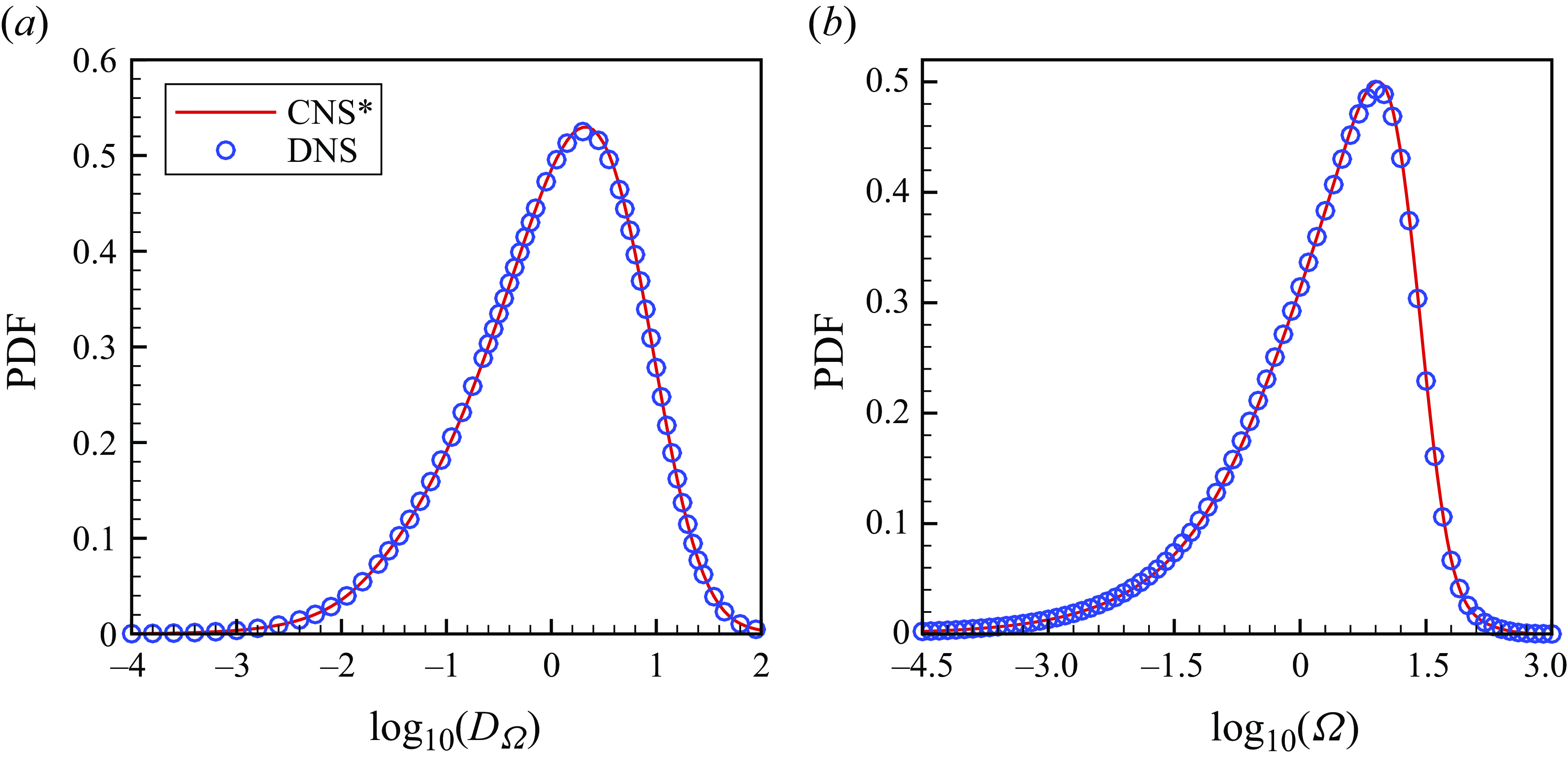
Figure 3. The PDFs of (a) the enstrophy dissipation rate $D_\Omega (x,y,t)$ and (b) the enstrophy $\Omega (x,y,t)$ of the 2-D turbulent Kolmogorov flow, where the integration is taken in $(x,y)\in [0,2\pi )^2$ and $t \in [100, 300]$ : CNS $^*$ (red line) and DNS (blue circles).

Figure 4. (a) Time-averaged kinetic energy spectra $\langle E_k \rangle _{t}$ of the 2-D turbulent Kolmogorov flow where the black dashed line corresponds to the $-5/3$ power law and the black dash-dot line denotes the wavenumber of external force $k=n_K=16$ . (b) Spatio–temporal-averaged scale-to-scale energy fluxes $\langle \Pi ^{[l]} \rangle$ of the 2-D turbulent Kolmogorov flow where the black dashed line denotes $\langle \Pi ^{[l]} \rangle =0$ and the black dash-dot line denotes the forcing scale $l=l_f=\pi /n_K=0.196$ . Red solid line denotes the CNS $^*$ result. Blue circles denote the DNS result.

Figure 5. Spatio–temporal-averaged scale-to-scale enstrophy fluxes $\langle \Pi _\Omega ^{[l]} \rangle$ of the 2-D turbulent Kolmogorov flow where the black dashed line denotes $\langle \Pi _\Omega ^{[l]} \rangle =0$ and the black dash-dot line denotes the forcing scale $l=l_f=\pi /n_K=0.196$ . Red solid line denotes the CNS $^*$ result. Blue circles denote the DNS result.

For the difference between the velocity fields given by CNS $^*$ and DNS, say, $\Delta {\boldsymbol u}= {\boldsymbol u}_{ {CNS}^*}-{\boldsymbol u}_{ {DNS}}$ , here we focus on the time evolution of the spatially averaged error/uncertainty energy $\langle E_{\Delta }\rangle _A=\langle |\Delta {\boldsymbol u}|^2/2 \rangle _A$ (Boffetta & Musacchio 2001, 2017; Ge et al. 2023), as well as the kinetic energy spectra of $\Delta {\boldsymbol u}$ at different times, see figure S1 in the supplementary material. It reveals the exponential growth of thermal fluctuation and/or stochastic environmental noise, since the thermal fluctuation and/or stochastic environmental noise added via (2.7) in CNS $^*$ is larger than the numerical noise in DNS.

Note that our CNS $^{*}$ result with negligible artificial numerical noise contains thermal fluctuation and/or stochastic environmental noise, but the DNS result without thermal fluctuation and/or stochastic environmental noise has rapidly become badly polluted by artificial numerical noise. The foregoing comparisons collectively provide evidence that artificial numerical noise in DNS is approximately equivalent to thermal fluctuation and/or stochastic environmental noise, at least for the 2-D turbulent Kolmogorov flow considered in this paper. This means that the artificial numerical noise in DNS has physical significance, which provides us with a really positive perspective on artificial numerical noise in the numerical simulation of turbulence.

3.2. Physical significance of artificial numerical noise of DNS

Given that the artificial numerical noise in DNS is approximately equivalent to thermal fluctuation and/or stochastic environmental noise, artificial numerical noise can thus be regarded from a totally different physical perspective: different sources of artificial numerical noise in DNS, arising from different algorithms, different spatial meshes, different time steps, etc., correspond to different thermal fluctuations and/or stochastic environmental noises. From this physical viewpoint of artificial numerical noise, DNS results given by various numerical algorithms with different levels of artificial numerical noise correspond to different turbulent flows under different levels of physical disturbances such as thermal fluctuation and/or stochastic environmental noise: all of them could be correct and have physical meaning.

Figure 6. Time histories of the spatially averaged (a) kinetic energy dissipation rate $\langle D\rangle _A$ and (b) enstrophy dissipation rate $\langle D_{\Omega }\rangle _A$ of the 2-D turbulent Kolmogorov flow, given by DNS using the following four uniform meshes: $1024\times 1024$ (red line), $512\times 512$ (black line), $256\times 256$ (blue line) and $128\times 128$ (orange line).

Figure 7. The PDFs of (a) the kinetic energy dissipation rate $D(x,y,t)$ and (b) the kinetic energy $E(x,y,t)$ of the 2-D turbulent Kolmogorov flow, given by DNS using the following four uniform meshes: $1024\times 1024$ (red line), $512\times 512$ (black circle), $256\times 256$ (blue inverted triangle) and $128\times 128$ (orange triangle).

Figure 8. (a) Time-averaged kinetic energy spectra $\langle E_k \rangle _{t}$ of the 2-D turbulent Kolmogorov flow. The black dashed line corresponds to the -5/3 power law and the black dash-dot line denotes the wavenumber of external force $k=n_K=16$ . (b) Spatio–temporal-averaged scale-to-scale energy fluxes $\langle \Pi ^{[l]} \rangle$ of the 2-D turbulent Kolmogorov flow where the black dashed line denotes $\langle \Pi ^{[l]} \rangle =0$ and the black dash-dot line denotes the forcing scale $l=l_f=\pi /n_K=0.196$ . In both (a) and (b), the results were obtained using DNS on $1024\times 1024$ (red solid line), $512\times 512$ (black circle), $256\times 256$ (blue inverted triangle) and $128\times 128$ (orange triangle) uniform meshes.

For example, we can similarly obtain different DNS results by means of the same strategy as mentioned previously, i.e. 4th-order Runge–Kutta method with time step $\Delta t=10^{-4}$ in double precision, as well as the same pseudo-spectral method in space but using the three different uniform meshes, i.e. $512\times 512$ , $256\times 256$ and $128\times 128$ , corresponding to different levels of spatial truncation error. As shown in figure 6, the time histories of the spatially averaged kinetic energy dissipation rate $\langle D\rangle _A$ and enstrophy dissipation rate $\langle D_{\Omega }\rangle _A$ given by DNS using the previously mentioned three different uniform meshes are almost the same as those given by DNS using the finest uniform mesh $1024\times 1024$ , especially when $t\gt 100$ corresponding to a relatively stable state of turbulence. Besides, the PDFs of kinetic energy dissipation rate $D(x,y,t)$ and kinetic energy $E(x,y,t)$ are also almost the same, as shown in figure 7(a) and 7(b), respectively. Similarly, the PDFs of the enstrophy dissipation rate $D_\Omega (x,y,t)$ and the enstrophy $\Omega (x,y,t)$ given by different uniform meshes also agree quite well (see figure S2 in the supplementary material). As shown in figure 8(a), there exists no obvious difference between the temporal averaged kinetic energy spectra $\langle E_k \rangle _{t}$ obtained via the four meshes: all satisfy the Kolmogorov $-5/3$ power law. Figure 8(b) shows that the spatio–temporal-averaged scale-to-scale energy fluxes $\langle \Pi ^{[l]} \rangle$ obtained via the different meshes mostly agree well with each other, except at $l\approx 10^{-1}$ for the uniform $128\times 128$ mesh that is too sparse to accurately describe the small-scale turbulent flow in detail. However, even so, all of them lead correctly to the physical conclusion that the energy cascade is inverse, i.e. directed from small scale to large scale. In addition, all the spatio–temporal-averaged scale-to-scale enstrophy fluxes $\langle \Pi _\Omega ^{[l]} \rangle$ given by these different uniform meshes display the direct enstrophy cascade (see figure S3 in the supplementary material). The foregoing indicate that the statistical results given by DNS using the four uniform meshes of different resolution agree quite well for the 2-D turbulent Kolmogorov flow under consideration. This is indeed a very surprising result.

Traditionally, DNS has been widely regarded as providing ‘reliable’ benchmark solutions of turbulence as long as the grid spacing is fine enough, say, less than the enstrophy dissipative scale for 2-D turbulence (Boffetta & Ecke 2012), and the time step is sufficiently small, say, satisfying the Courant–Friedrichs–Lewy condition, i.e. Courant number ${\lt } 1$ (Courant, Friedrichs & Lewy 1928). In principle, these two conditions must be satisfied for DNS of turbulence. As shown in figure 6(b), all spatially averaged enstrophy dissipation rates $\langle D_{\Omega }\rangle _A(t)$ given by DNS using the four different meshes are almost the same when $t\gt 100$ . Thus, integrated over $(x,y)\in [0,2\pi )^2$ and $t \in [100, 300]$ , we obtain almost the same spatio–temporal-averaged enstrophy dissipation rates $\langle D_{\Omega }\rangle =3.5$ for all DNS results using the four different uniform meshes, and the corresponding enstrophy dissipative scale (Boffetta & Musacchio 2010) is

(3.1) \begin{equation} \langle \eta _{\Omega } \rangle \approx Re^{-1/2}\langle D_{\Omega } \rangle ^{-1/6}=0.018. \end{equation}

Thus, we have the corresponding grid spacing $\Delta _{1024}=2\pi /1024\approx 0.34\langle \eta _{\Omega } \rangle$ for the $1024\times 1024$ mesh, $\Delta _{512}\approx 0.68\langle \eta _{\Omega } \rangle$ for the $512\times 512$ mesh, $\Delta _{256}\approx 1.36\langle \eta _{\Omega } \rangle$ for the $256 \times 256$ mesh and $\Delta _{128}\approx 2.73\langle \eta _{\Omega } \rangle$ for the $128\times 128$ mesh. It should be emphasised that, although the grid spacing is fine enough for only the two uniform meshes $1024\times 1024$ and $512\times 512$ , all the statistical results obtained using DNS on the different meshes agree quite well with each other, even if the grid spacing $\Delta _{128}$ is even 2.73 times larger than the enstrophy dissipative scale $\langle \eta _{\Omega } \rangle$ . It is hard to explain this kind of agreement in the traditional frame of the DNS.

However, the previously mentioned phenomena can be fully explained by considering the physical meaning of artificial numerical noise of DNS, revealed in § 3.1. Note that the DNS algorithms using the four different uniform meshes have different levels of artificial numerical noise, which are approximately equivalent to different levels of thermal fluctuation and/or stochastic environmental noise. Therefore, each DNS result corresponds to a 2-D turbulent Kolmogorov flow under a particular level of thermal fluctuation and/or stochastic environmental noise: their spatio–temporal trajectories are certainly different, but all of them have physical meaning. In other words, all are physically correct! So, it is meaningless to try to say which one among them is better given that all of them are correct in physics, corresponding to a turbulent flow under a kind of thermal fluctuation and/or stochastic environmental noise.

Note that, for the 2-D turbulent Kolmogorov flow under consideration, all the statistical results given by DNS using the four different uniform meshes (and even different time steps) agree well, indicating that statistical stability has been achieved and the simulations are insensitive to different levels of disturbance. It should be emphasised that, for turbulent flow that is statistically stable, one can use even a sparse $128 \times 128$ mesh (i.e. requiring much less CPU time) to gain almost the same statistical results as those on the finest $1024\times 1024$ mesh. Thus, statistical stability is very important for numerical simulation of turbulence in practice. This is exactly the reason why Liao (2023) proposed the so-called ‘modified fourth Clay millennium problem’:

• ‘The existence, smoothness and statistic stability of the Navier–Stokes equation: Can we prove the existence, smoothness and statistic stability (or instability) of the solution of the Navier–Stokes equation with physically proper boundary and initial conditions?’

Unfortunately, such kind of statistic stability does not always exist for all turbulent flows, as illustrated as follows.

3.3. An example of turbulence with statistic instability

Figure 9. (a,b) Temperature departure from a linear variation background ( $\theta$ ) at time $t=250$ of 2-D turbulent RBC for Rayleigh number $Ra=5\times 10^7$ , Prandtl number $Pr=6.8$ and aspect ratio $\Gamma =2\sqrt {2}$ , given by DNS with different time steps: (a) non-shearing vortical/roll-like flow given by $\Delta t=1.1\times 10^{-3}$ and (b) zonal flow given by $\Delta t=10^{-3}$ . (c) Final flow type of the turbulent RBC versus time step $\Delta t$ of DNS for the same RBC: either non-shearing vortical/roll-like flow (blue circles) or zonal flow (red squares).

Let us recall that, by means of CNS, Qin & Liao (2022) investigated the large-scale influence of numerical noise as tiny artificial stochastic disturbances on sustained turbulence, i.e. 2-D turbulent Rayleigh–Bénard convection (RBC) for aspect ratio $\Gamma = 2\sqrt {2}$ , Prandtl number $Pr$ = 6.8 (corresponding to water at room temperature, 20  $^{\circ }$ C) and Rayleigh number $Ra = 6.8 \times 10^{8}$ (corresponding to a turbulent state). It was found (Qin & Liao 2022) that the CNS benchmark solution always sustains a non-shearing vortical/roll-like convection throughout the whole simulation; however, the DNS result is a kind of vortical/roll-like convection at the beginning but finally turns into a kind of zonal flow. The two distinct types of turbulent convection are also confirmed by Wang, Goluskin & Lohse (2023). This illustrated that numerical noise as tiny artificial stochastic disturbance could lead to the simulated turbulence experiencing large-scale deviations not only in spatio–temporal trajectories but also even in statistics and type of flow. This is a good example of turbulence having statistic instability.

To show such kind of statistic instability in more detail, let us further consider here the same 2-D turbulent RBC, governed by the same mathematical equations subject to the same initial/boundary conditions with the same physical parameters as those used by Qin & Liao (2022), except for a smaller Rayleigh number $Ra=5\times 10^7$ . The same DNS algorithm using the same uniform mesh $1024\times 1024$ as that by Qin & Liao (2022) is adapted but with various time steps, which correspond to different levels of artificial numerical noise that are approximately equivalent to different levels of thermal fluctuation and/or stochastic environmental noise, as verified in § 3.1.

It is found that the flow type and the corresponding statistical results given by DNS are rather sensitive to the value of time step $\Delta t$ . For example, the time step $\Delta t=1.1\times 10^{-3}$ gives a non-shearing vortical/roll-like flow, but the time step $\Delta t=10^{-3}$ corresponds to a zonal flow, as shown in figure 9(a,b). It should be emphasised that the difference between the two time steps is merely $10^{-4}$ . Note that the final flow type of the 2-D turbulent RBC is rather sensitive to the time step $\Delta t$ of DNS, as shown in figure 9(c): as $\Delta t$ varies from $10^{-4}$ to $1.5\times 10^{-3}$ with uniform interval $10^{-4}$ , where the final flow type consistently fluctuates between non-shearing vortical/roll-like flow and zonal flow, the statistics of the corresponding turbulent flow fluctuate, i.e. promote statistical instability.

Note that artificial numerical noise of DNS is approximately equivalent to thermal fluctuation and/or stochastic environmental noise, as verified in § 3.1. Therefore, each of our DNS results given by different time steps corresponds to a kind of turbulent flow under a different level of thermal fluctuation and/or stochastic environmental noise (regardless of its different statistics), and thus has proper physical meaning, no matter whether the flow type is non-shearing vortical/roll-like flow or zonal flow.

4. Concluding remarks and discussions

Using CNS, we provide rigorous evidence that, for DNS of turbulence, artificial numerical noise is approximately equivalent to thermal fluctuation and/or stochastic environmental noise. This reveals the physical significance of artificial numerical noise in DNS of turbulence governed by the NS equations. In other words, the results produced by DNS on different numerical meshes should correspond to turbulent flows under different levels of internal/external physical disturbances. More importantly, all could have physical meaning even if their statistics are quite different, so long as these equivalent disturbances are reasonable and practical in physics. This provides a positive perspective on artificial numerical noise in DNS of turbulence.

Note that, by means of DNS itself, it is impossible to verify that artificial numerical noise in DNS is approximately equivalent to thermal fluctuation and/or stochastic environmental noise, because the DNS result rapidly becomes badly polluted by its inherent numerical noise. This illustrates that CNS, whose artificial numerical noise is negligible over a finite, sufficiently long time interval, can indeed provide us with a useful tool by which to investigate the propagation and evolution of artificial/physical micro-level disturbances and their large-scale influence on turbulence.

Similarly, due to the butterfly effect of chaos, artificial numerical noise will enlarge quickly to macro level of a chaotic system. Thus, the foregoing conclusions should also hold in general for a chaotic system; in other words, the artificial numerical noise of every chaos should be equivalent to its physical and/or stochastic environmental noise.

Data-driven artificial intelligence (AI) and machine learning (ML) have been used widely in fluid mechanics. Note that all data contain noise and all algorithms in ML and/or AI are likely to introduce some artificial noise. Obviously, the physical significance of artificial numerical noise in DNS could provide a new viewpoint for data-driven AI and ML in fluid mechanics.

It is a well-known phenomenon in computational fluid dynamics (CFD) that numerical simulations of a turbulent flow given by various algorithms are quite different from each other and from the corresponding physical experiment when its experimental result has not been announced, but generally agree well with the experimental result as soon as it is announced. The conventional explanation for this ‘famous’ phenomenon is that those simulations that exhibit obvious deviations from the physical experimental results must be wrong, primarily because the numerical algorithm and/or spatial mesh are simply not good enough, leading to too high a level of artificial numerical noise to obtain the ‘correct’ numerical results. However, according to the new viewpoint about artificial numerical noise revealed in this paper, many (or even all) of these numerical results might be correct in physics, even if there exist huge deviations between them (as illustrated in § 3.3, see figure 9), because their internal/external physical disturbances might be quite different but the corresponding physical experiment simply corresponds to one special case of physical disturbance. Hopefully, the physical significance of artificial numerical noise as a really positive viewpoint revealed in this paper could be of benefit to greatly deepen our understanding about the so-called ‘crisis of reproducibility’ for CFD (Baker 2016).

Note that, if thermal fluctuation and/or stochastic environmental noise is not considered, the CNS result retains the same spatial symmetry as the initial condition throughout the whole time interval $t\in [0,300]$ , and, besides, its statistics are obviously different from those given by DNS. This conclusion is clear and obvious from our previous publications (Qin et al. 2024; Liao & Qin 2025) about the 2-D turbulent Kolmogorov flow. However, as illustrated in this paper, when considering thermal fluctuation and/or stochastic environmental noise, both of CNS (with thermal fluctuation and/or environmental disturbance) and DNS (that is badly polluted by numerical noise, but without thermal fluctuation and/or environmental disturbance) give the same statistics, strongly suggesting that there should exist some relationship between numerical noise and thermal fluctuation and/or environmental disturbance. In this meaning, we highly suggest that the numerical noise should be approximately equivalent to thermal fluctuation or stochastic environmental disturbance, although further detailed investigations are certainly necessary in the future.

Note that a few molecular simulations using molecular-gas-dynamics (MGD) technique (McMullen et al. 2022) or unified stochastic particle (USP) (Ma et al. 2024) demonstrated that thermal fluctuations might significantly influence the small-scale statistics of turbulence, leading to a $k$ scaling in the dissipation range of 2-D turbulent energy spectrum and a $k^2$ scaling in the 3-D case. This phenomenon has been confirmed by Landau–Lifshitz–Navier–Stokes (LLNS) equations (Bandak et al. 2022) and/or fluctuating hydrodynamics (Bell et al. 2022) but not by NS equations. Note that DNS results of NS or LLNS equations are badly polluted by artificial numerical noises, as illustrated by Qin et al. (2024). Although LLNS equations (Landau & Lifshitz 1959) are not as widely used as NS equations, it should be very interesting in future to use CNS to solve LLNS equations so as to study influence of thermal fluctuation on turbulence with negligible numerical noise.