


1 Introduction
For
 $\alpha>0$
and nonnegative
$\alpha>0$
and nonnegative
 $f\in L^1(\mathbb {S}^n)$
with positive integral, we are interested in finding a weak solution to the Monge–Ampére equation
$f\in L^1(\mathbb {S}^n)$
with positive integral, we are interested in finding a weak solution to the Monge–Ampére equation
 $$ \begin{align} u^{\frac1\alpha}\det(\bar{\nabla}^2_{ij} u+u\bar{g}_{ij})=f, \end{align} $$
or in other words, a weak solution to Lutwak’s
 $L^p$
-Minkowski problem on
$L^p$
-Minkowski problem on
 $S^n$
when
$S^n$
when
 $-n-1<p<1$
for
$-n-1<p<1$
for
 $p=1-\frac 1\alpha $
where
$p=1-\frac 1\alpha $
where
 $\bar {\nabla }$
is the Levi-Civita connection of
$\bar {\nabla }$
is the Levi-Civita connection of
 $\mathbb {S}^n$
,
$\mathbb {S}^n$
,
 $\bar {g}_{ij}$
, with
$\bar {g}_{ij}$
, with
 $\bar {g}$
being the induced round metric on the unit sphere. By a weak (Alexandrov) solution, we mean the following: Given a nontrivial finite Borel measure
$\bar {g}$
being the induced round metric on the unit sphere. By a weak (Alexandrov) solution, we mean the following: Given a nontrivial finite Borel measure
 $\mu $
on
$\mu $
on
 $\mathbb {S}^n$
(for example,
$\mathbb {S}^n$
(for example,
 $d\mu =f\,d\theta $
for the Lebesgue measure
$d\mu =f\,d\theta $
for the Lebesgue measure
 $\theta $
on
$\theta $
on
 $S^n$
and the f in (1.1)), find a convex body
$S^n$
and the f in (1.1)), find a convex body
 $\Omega \subset \Bbb R^{n+1}$
with
$\Omega \subset \Bbb R^{n+1}$
with
 $o\in \Omega $
such that
$o\in \Omega $
such that
 $$ \begin{align} d\mu=u^{\frac1\alpha}\,dS_\Omega, \end{align} $$
where
 $u(x)=\max _{z\in \Omega }\langle x,z\rangle $
is the support function and
$u(x)=\max _{z\in \Omega }\langle x,z\rangle $
is the support function and
 $S_\Omega $
is the surface area measure of
$S_\Omega $
is the surface area measure of
 $\Omega $
(see [Reference Schneider45]). If
$\Omega $
(see [Reference Schneider45]). If
 $\partial \Omega $
is
$\partial \Omega $
is
 $C^2_+$
, then
$C^2_+$
, then
 $$ \begin{align*}dS_\Omega=\det(\bar{\nabla}^2_{ij} u+u\bar{g}_{ij})d\theta=K^{-1}d\theta, \end{align*} $$
where
 $K(x)$
is the Gaussian curvature at the point of
$K(x)$
is the Gaussian curvature at the point of
 $\partial \Omega $
where
$\partial \Omega $
where
 $x\in S^n$
is the exterior unit normal (see [Reference Schneider45]). Concerning the regularity of the solution of (1.1), if
$x\in S^n$
is the exterior unit normal (see [Reference Schneider45]). Concerning the regularity of the solution of (1.1), if
 $f\in C^{0,\beta }(S^n)$
and u are positive, then u is
$f\in C^{0,\beta }(S^n)$
and u are positive, then u is
 $C^{2,\beta }$
according to Caffarelli’s regularity theory in [Reference Caffarelli15, Reference Caffarelli16]. On the other hand, even if f is positive and continuous for
$C^{2,\beta }$
according to Caffarelli’s regularity theory in [Reference Caffarelli15, Reference Caffarelli16]. On the other hand, even if f is positive and continuous for
 $\alpha>\frac 1n$
, there might exist weak solution where
$\alpha>\frac 1n$
, there might exist weak solution where
 $u(x)=0$
for some
$u(x)=0$
for some
 $x\in S^n$
and u is not even
$x\in S^n$
and u is not even
 $C^1$
according to Example 4.2 in [Reference Bianchi, Böröczky and Colesanti7]. Moreover, even if
$C^1$
according to Example 4.2 in [Reference Bianchi, Böröczky and Colesanti7]. Moreover, even if
 $f\in C^{0,\beta }(S^n)$
is positive, it is possible that
$f\in C^{0,\beta }(S^n)$
is positive, it is possible that
 $u(x)=0$
for some
$u(x)=0$
for some
 $x\in S^n$
for
$x\in S^n$
for
 $\alpha>\frac 1n$
, but Choi, Kim, and Lee [Reference Choi, Kim and Lee19] still managed to obtain some regularity results in this case.
$\alpha>\frac 1n$
, but Choi, Kim, and Lee [Reference Choi, Kim and Lee19] still managed to obtain some regularity results in this case.
The case
 $\alpha =\frac 1{n+2}$
of the Monge–Ampére equation (1.1) is the critical case when the left-hand side of (1.1) is invariant under linear transformations of
$\alpha =\frac 1{n+2}$
of the Monge–Ampére equation (1.1) is the critical case when the left-hand side of (1.1) is invariant under linear transformations of
 $\Omega $
, and the case
$\Omega $
, and the case
 $\alpha =1$
is the so-called logarithmic Minkowski problem posed by Firey [Reference Firey23]. Setting
$\alpha =1$
is the so-called logarithmic Minkowski problem posed by Firey [Reference Firey23]. Setting
 $p=1-\frac 1\alpha <1$
, the Monge–Ampére equation (1.1) is Lutwak’s
$p=1-\frac 1\alpha <1$
, the Monge–Ampére equation (1.1) is Lutwak’s
 $L^p$
-Minkowski problem
$L^p$
-Minkowski problem
 $$ \begin{align} u^{1-p}\det(\bar{\nabla}^2_{ij} u+u\bar{g}_{ij})=f. \end{align} $$
In this notation, (1.2) reads as
 $$ \begin{align} d\mu=u^{1-p}\,dS_\Omega; \end{align} $$
that equation makes sense for any
 $p\in \Bbb R$
. Within the rapidly developing
$p\in \Bbb R$
. Within the rapidly developing
 $L^p$
-Brunn–Minkowski theory (where
$L^p$
-Brunn–Minkowski theory (where
 $p=1$
is the classical case originating from Minkowski’s oeuvre) initiated by Lutwak [Reference Lutwak39–Reference Lutwak41], if
$p=1$
is the classical case originating from Minkowski’s oeuvre) initiated by Lutwak [Reference Lutwak39–Reference Lutwak41], if
 $p>1$
and
$p>1$
and
 $p\neq n+1$
, then Hug, Lutwak, Yang, and Zhang [Reference Hug, Lutwak, Yang and Zhang30] (improving on Chou and Wang [Reference Chou and Wang20]) prove that (1.4) has an Alexandrov solution if and only if the
$p\neq n+1$
, then Hug, Lutwak, Yang, and Zhang [Reference Hug, Lutwak, Yang and Zhang30] (improving on Chou and Wang [Reference Chou and Wang20]) prove that (1.4) has an Alexandrov solution if and only if the
 $\mu $
is not concentrated onto any closed hemisphere, and the solution is unique. We note that there are examples in [Reference Guan and Lin25] (see also [Reference Hug, Lutwak, Yang and Zhang30]) and show that if
$\mu $
is not concentrated onto any closed hemisphere, and the solution is unique. We note that there are examples in [Reference Guan and Lin25] (see also [Reference Hug, Lutwak, Yang and Zhang30]) and show that if
 $1<p<n+1$
, then it may happen that the density function f is a positive continuous in (1.3) and
$1<p<n+1$
, then it may happen that the density function f is a positive continuous in (1.3) and
 $o\in \partial K$
holds for the unique Alexandrov solution, and actually Bianchi, Böröczky, and Colesanti [Reference Bianchi, Böröczky and Colesanti7] exhibit an example that
$o\in \partial K$
holds for the unique Alexandrov solution, and actually Bianchi, Böröczky, and Colesanti [Reference Bianchi, Böröczky and Colesanti7] exhibit an example that
 $o\in \partial K$
even if the density function f is a positive continuous in (1.3) assuming
$o\in \partial K$
even if the density function f is a positive continuous in (1.3) assuming
 $-n-1<p<1$
.
$-n-1<p<1$
.
In the case
 $p\in (0,1)$
(or equivalently,
$p\in (0,1)$
(or equivalently,
 $\alpha>1$
), if the measure
$\alpha>1$
), if the measure
 $\mu $
is not concentrated onto any great subsphere of
$\mu $
is not concentrated onto any great subsphere of
 $S^n$
, then Chen, Li, and Zhu [Reference Chen, Li and Zhu17] prove that there exists an Alexandrov solution
$S^n$
, then Chen, Li, and Zhu [Reference Chen, Li and Zhu17] prove that there exists an Alexandrov solution
 $K\in \mathcal {K}_o^n$
of (1.4) using a variational argument (see also [Reference Bianchi, Böröczky, Colesanti and Yang8]). We note that for
$K\in \mathcal {K}_o^n$
of (1.4) using a variational argument (see also [Reference Bianchi, Böröczky, Colesanti and Yang8]). We note that for
 $p\in (0,1)$
and
$p\in (0,1)$
and
 $n\geq 2$
, no complete characterization of
$n\geq 2$
, no complete characterization of
 $L^p$
-surface area measures is known (see [Reference Böröczky and Trinh12] for the case
$L^p$
-surface area measures is known (see [Reference Böröczky and Trinh12] for the case
 $n=1$
, and [Reference Bianchi, Böröczky, Colesanti and Yang8, Reference Saroglou43] for partial results about the case when
$n=1$
, and [Reference Bianchi, Böröczky, Colesanti and Yang8, Reference Saroglou43] for partial results about the case when
 $n\geq 2$
and the support of
$n\geq 2$
and the support of
 $\mu $
is contained in a great subsphere of
$\mu $
is contained in a great subsphere of
 $S^n$
).
$S^n$
).
Concerning the case
 $p=0$
(or equivalently,
$p=0$
(or equivalently,
 $\alpha =1$
), the still open logarithmic Minkowski problem (1.3) or (1.4) was posed by Firey [Reference Firey23] in 1974. The paper [Reference Böröczky, Lutwak, Yang and Zhang11] characterized even measures
$\alpha =1$
), the still open logarithmic Minkowski problem (1.3) or (1.4) was posed by Firey [Reference Firey23] in 1974. The paper [Reference Böröczky, Lutwak, Yang and Zhang11] characterized even measures
 $\mu $
such that (1.4) has an even solution for
$\mu $
such that (1.4) has an even solution for
 $p=0$
by the so-called subspace concentration condition (see (a) and (b) in Theorem 1.1). In general, Chen, Li, and Zhu [Reference Chen, Li and Zhu18] proved that if a nontrivial finite Borel measure
$p=0$
by the so-called subspace concentration condition (see (a) and (b) in Theorem 1.1). In general, Chen, Li, and Zhu [Reference Chen, Li and Zhu18] proved that if a nontrivial finite Borel measure
 $\mu $
on
$\mu $
on
 $S^{n-1}$
satisfies the same subspace concentration condition, then (1.4) has a solution for
$S^{n-1}$
satisfies the same subspace concentration condition, then (1.4) has a solution for
 $p=0$
. On the other hand, Böröczky and Hegedus [Reference Böröczky and Hegedűs10] provide conditions on the restriction of the
$p=0$
. On the other hand, Böröczky and Hegedus [Reference Böröczky and Hegedűs10] provide conditions on the restriction of the
 $\mu $
in (1.4) to a pair of antipodal points.
$\mu $
in (1.4) to a pair of antipodal points.
If
 $-n-1<p<0$
(or equivalently,
$-n-1<p<0$
(or equivalently,
 $\frac 1{n+2}<\alpha <1$
) and
$\frac 1{n+2}<\alpha <1$
) and
 $f\in L_{\frac {n+1}{n+1+p}}(S^{n})$
in (1.3), then (1.3) has a solution according to [Reference Bianchi, Böröczky, Colesanti and Yang8]. For a rather special discrete measure
$f\in L_{\frac {n+1}{n+1+p}}(S^{n})$
in (1.3), then (1.3) has a solution according to [Reference Bianchi, Böröczky, Colesanti and Yang8]. For a rather special discrete measure
 $\mu $
satisfying that
$\mu $
satisfying that
 $\mu $
is not concentrated on any closed hemisphere and any n unit vectors in the support of
$\mu $
is not concentrated on any closed hemisphere and any n unit vectors in the support of
 $\mu $
are independent, Zhu [Reference Zhu47] solves the
$\mu $
are independent, Zhu [Reference Zhu47] solves the
 $L^p$
-Minkowski problem (1.4) for
$L^p$
-Minkowski problem (1.4) for
 $p<0$
. The
$p<0$
. The
 $p=-n-1$
(or equivalently,
$p=-n-1$
(or equivalently,
 $\alpha =\frac 1{n+2}$
) case of the
$\alpha =\frac 1{n+2}$
) case of the
 $L^p$
-Minkowski problem is the critical case because its link with the
$L^p$
-Minkowski problem is the critical case because its link with the
 $\mathrm {SL}(n)$
invariant centro-affine curvature whose reciprocal is
$\mathrm {SL}(n)$
invariant centro-affine curvature whose reciprocal is
 $u^{n+2}\det (\bar {\nabla }^2_{ij} u+u\bar {g}_{ij})$
(see [Reference Hug29] or [Reference Ludwig38]). For positive results concerning the critical case
$u^{n+2}\det (\bar {\nabla }^2_{ij} u+u\bar {g}_{ij})$
(see [Reference Hug29] or [Reference Ludwig38]). For positive results concerning the critical case
 $p=-n-1$
, see, for example, [Reference Guang, Li and Wang28, Reference Jian, Lu and Zhu34], and for obstructions for a solution, see, for example, [Reference Chou and Wang20, Reference Du22].
$p=-n-1$
, see, for example, [Reference Guang, Li and Wang28, Reference Jian, Lu and Zhu34], and for obstructions for a solution, see, for example, [Reference Chou and Wang20, Reference Du22].
In the super-critical case
 $p<-n-1$
(or equivalently,
$p<-n-1$
(or equivalently,
 $\alpha <\frac 1{n+2}$
), there is a recent important work by Li, Guang, and Wang [Reference Guang, Li and Wang27] proving that for any positive
$\alpha <\frac 1{n+2}$
), there is a recent important work by Li, Guang, and Wang [Reference Guang, Li and Wang27] proving that for any positive
 $C^2$
function f, there exists a
$C^2$
function f, there exists a
 $C^4$
solution of (1.3). See also [Reference Du22] for non-existence examples.
$C^4$
solution of (1.3). See also [Reference Du22] for non-existence examples.
The main contribution of this paper is to provide a very natural argument based on anisotropic flows developed by Andrews [Reference Andrews4] to handle the case
 $-n-1<p<1$
, or equivalently, the case
$-n-1<p<1$
, or equivalently, the case
 $\frac 1{n+2}<\alpha <\infty $
.
$\frac 1{n+2}<\alpha <\infty $
.
Entropy functional. For any convex body
 $\Omega $
, a fixed positive function f on
$\Omega $
, a fixed positive function f on
 $\mathbb {S}^n$
and
$\mathbb {S}^n$
and
 $\alpha \in (0, \infty )$
, define
$\alpha \in (0, \infty )$
, define
 $$ \begin{align} \mathcal{E}_{\alpha, f} (\Omega) := \sup_{z\in\Omega}{\mathcal E}_{\alpha, f}(\Omega,z), \end{align} $$
where
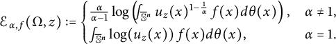 $$ \begin{align} {\mathcal E}_{\alpha, f}(\Omega,z) := \begin{cases} \frac{\alpha}{\alpha-1}\log\left(\frac{\ \ }{\ \ }{\hskip -0.4cm}\int_{\mathbb{S}^n} u_{z}(x)^{1-\frac1\alpha}\,f(x) d\theta(x)\right),&\alpha\neq 1,\\ \hspace{3pt}\frac{\ \ }{\ \ }{\hskip -0.4cm}\int_{\mathbb{S}^n} \log(u_{z}(x))\, f(x) d\theta(x),&\alpha=1. \end{cases} \end{align} $$
Here,
 $u_{z}(x):=\sup _{y\in \Omega }\left \langle y-z,x\right \rangle $
is the support function of
$u_{z}(x):=\sup _{y\in \Omega }\left \langle y-z,x\right \rangle $
is the support function of
 $\Omega $
in direction x with respect to
$\Omega $
in direction x with respect to
 $z_0$
and
$z_0$
and
 $\frac {\ \ }{\ \ }{\hskip -0.4cm}\int _{\mathbb {S}^n} h(x)\, d\theta (x)=\frac {1}{\omega _n} \int _{\mathbb {S}^n} h(x)$
with
$\frac {\ \ }{\ \ }{\hskip -0.4cm}\int _{\mathbb {S}^n} h(x)\, d\theta (x)=\frac {1}{\omega _n} \int _{\mathbb {S}^n} h(x)$
with
 $\omega _n$
being the surface area of
$\omega _n$
being the surface area of
 $\mathbb {S}^n$
and
$\mathbb {S}^n$
and
 $\theta $
is the Lebesgue measure on
$\theta $
is the Lebesgue measure on
 $S^n$
. When
$S^n$
. When
 $\alpha =1$
and
$\alpha =1$
and
 $f(x)\equiv 1$
, then the above quantity agrees with the entropy in [Reference Guan and Ni26], first introduced by Firey [Reference Firey23] for the centrally symmetric
$f(x)\equiv 1$
, then the above quantity agrees with the entropy in [Reference Guan and Ni26], first introduced by Firey [Reference Firey23] for the centrally symmetric
 $\Omega $
. General integral quantities were studied by Andrews in [Reference Andrews2, Reference Andrews4]. Here, we shall assume that
$\Omega $
. General integral quantities were studied by Andrews in [Reference Andrews2, Reference Andrews4]. Here, we shall assume that
 $\frac {\ \ }{\ \ }{\hskip -0.4cm}\int _{\mathbb {S}^n} f(x)\, d\theta (x)=1$
, namely,
$\frac {\ \ }{\ \ }{\hskip -0.4cm}\int _{\mathbb {S}^n} f(x)\, d\theta (x)=1$
, namely,
 $\frac 1{\omega _n}\,f(x)d\theta (x)$
is a probability measure. For the special case
$\frac 1{\omega _n}\,f(x)d\theta (x)$
is a probability measure. For the special case
 $f\equiv 1$
,
$f\equiv 1$
,
 $\mathcal {E}_{\alpha , f}(\Omega ) $
becomes the entropy
$\mathcal {E}_{\alpha , f}(\Omega ) $
becomes the entropy
 $\mathcal {E}_\alpha (\Omega )$
in [Reference Andrews, Guan and Ni6].
$\mathcal {E}_\alpha (\Omega )$
in [Reference Andrews, Guan and Ni6].
For positive
 $f\in C^{\infty }(\mathbb S^n)$
, consider the anisotropic flow for convex hypersurfaces
$f\in C^{\infty }(\mathbb S^n)$
, consider the anisotropic flow for convex hypersurfaces
 $\tilde X(\cdot , \tau ): M_{\tau }\to \mathbb {R}^{n+1}$
:
$\tilde X(\cdot , \tau ): M_{\tau }\to \mathbb {R}^{n+1}$
:
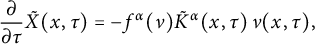 $$ \begin{align} \frac{\partial}{\partial \tau}\tilde X(x, \tau)= -f^{\alpha} (\nu) \tilde K^{\alpha}(x, \tau)\, \nu(x, \tau), \end{align} $$
where
 $\nu (x, \tau )$
is the unit exterior normal at
$\nu (x, \tau )$
is the unit exterior normal at
 $\tilde X(x, \tau )$
of
$\tilde X(x, \tau )$
of
 $\tilde M_\tau =\tilde X(M, \tau )$
, and
$\tilde M_\tau =\tilde X(M, \tau )$
, and
 $\tilde K(x,\tau )$
is the Gauss curvature of
$\tilde K(x,\tau )$
is the Gauss curvature of
 $\tilde M_\tau $
at
$\tilde M_\tau $
at
 $\tilde X(x,\tau )$
. Andrews [Reference Andrews4] proved that flow (1.7) contracts to a point under finite time if the initial hypersurface
$\tilde X(x,\tau )$
. Andrews [Reference Andrews4] proved that flow (1.7) contracts to a point under finite time if the initial hypersurface
 $M_0$
is strictly convex. Under a proper normalization, the normalized anisotropy flow of (1.7) is
$M_0$
is strictly convex. Under a proper normalization, the normalized anisotropy flow of (1.7) is
 $$ \begin{align} \frac{\partial}{\partial t}X(x, t)= -\frac{f^\alpha(\nu) K^{\alpha}(x, t)}{\frac{\ \ }{\ \ }{\hskip -0.4cm}\int_{\mathbb{S}^n}f^\alpha K^{\alpha-1}}\, \nu(x, t) +X(x,t). \end{align} $$
The basic observation is that a critical point for entropy
 $\mathcal {E}_{\alpha , f} (\Omega )$
defined in (1.5) under volume normalization is a solution to equation (1.1). The entropy is monotone along flow (1.8). One may view (1.1) is an “optimal solution” to this variational problem as the flow (1.8) provides a natural path to reach it. This approach was devised in [Reference Andrews, Böröczky, Guan and Ni5] with the aim to obtain convergence of the normalized flow (1.8). The main arguments in [Reference Andrews, Böröczky, Guan and Ni5] follows those in [Reference Andrews, Guan and Ni6, Reference Guan and Ni26] where convergence of isotropic flows by power of Gauss curvature (i.e.,
$\mathcal {E}_{\alpha , f} (\Omega )$
defined in (1.5) under volume normalization is a solution to equation (1.1). The entropy is monotone along flow (1.8). One may view (1.1) is an “optimal solution” to this variational problem as the flow (1.8) provides a natural path to reach it. This approach was devised in [Reference Andrews, Böröczky, Guan and Ni5] with the aim to obtain convergence of the normalized flow (1.8). The main arguments in [Reference Andrews, Böröczky, Guan and Ni5] follows those in [Reference Andrews, Guan and Ni6, Reference Guan and Ni26] where convergence of isotropic flows by power of Gauss curvature (i.e.,
 $f=1$
) was established. Unfortunately, the entropy point estimate in [Reference Andrews, Guan and Ni6, Reference Guan and Ni26] fails for general anisotropic flows except
$f=1$
) was established. Unfortunately, the entropy point estimate in [Reference Andrews, Guan and Ni6, Reference Guan and Ni26] fails for general anisotropic flows except
 $\frac {1}{n+2}<\alpha \le \frac {1}n$
[Reference Andrews4]. The convergence was obtained in [Reference Andrews, Böröczky, Guan and Ni5] assuming
$\frac {1}{n+2}<\alpha \le \frac {1}n$
[Reference Andrews4]. The convergence was obtained in [Reference Andrews, Böröczky, Guan and Ni5] assuming
 $M_0$
and f are invariant under a subgroup G of
$M_0$
and f are invariant under a subgroup G of
 $O(n+1)$
which has no fixed point. We note that an inverse Gauss curvature flow argument was considered by Bryan, Ivaki, and Scheuer [Reference Bryan, Ivaki and Scheuer14] to produce a origin-symmetric solution to (1.1).
$O(n+1)$
which has no fixed point. We note that an inverse Gauss curvature flow argument was considered by Bryan, Ivaki, and Scheuer [Reference Bryan, Ivaki and Scheuer14] to produce a origin-symmetric solution to (1.1).
Since we are only interested in finding a weak solution to (1.2), one only needs certain “weak” convergence of the flow (1.8). The key steps are to control diameter with entropy under appropriate conditions on measure
 $\mu =f d\theta $
on
$\mu =f d\theta $
on
 $\mathbb S^n$
and use monotonicity of entropy to produce a solution to (1.2). The following is our main result.
$\mathbb S^n$
and use monotonicity of entropy to produce a solution to (1.2). The following is our main result.
Theorem 1.1 For
 $\alpha>\frac 1{n+2}$
and finite nontrivial Borel measure
$\alpha>\frac 1{n+2}$
and finite nontrivial Borel measure
 $\mu $
on
$\mu $
on
 $\mathbb {S}^n$
,
$\mathbb {S}^n$
,
 $n\geq 1$
, there exists a weak solution of (1.2) provided the following holds:
$n\geq 1$
, there exists a weak solution of (1.2) provided the following holds:
-
(i) If
 $\alpha>1$
and
$\mu $
is not concentrated onto any great subsphere
$x^\bot \cap \mathbb {S}^n$
,
$x\in \mathbb {S}^n$
.
$\alpha>1$
and
$\mu $
is not concentrated onto any great subsphere
$x^\bot \cap \mathbb {S}^n$
,
$x\in \mathbb {S}^n$
. -
(ii) If
$\alpha =1$
and
$\mu $
satisfies that for any linear
$\ell $
-subspace
$L\subset \Bbb R^{n+1}$
with
$1\leq \ell \leq n$
, we have-
(a)
$\displaystyle \mu (L\cap \mathbb {S}^n)\leq \frac {\ell }{n+1}\cdot \mu (\mathbb {S}^n)$
; -
(b) equality in (a) for a linear
$\ell $
-subspace
$L\subset \Bbb R^{n+1}$
with
$1\leq d\leq n$
implies the existence of a complementary linear
$(n+1-\ell )$
-subspace
$\widetilde {L}\subset \Bbb R^{n+1}$
such that
$\mathrm {supp}\,\mu \subset L\cup \widetilde {L}$
.
-
-
(iii) If
$\frac 1{n+2}<\alpha <1$
and
$d\mu =f\,d\theta $
for nonnegative
$f\in L^{\frac {n+1}{n+2-\frac 1\alpha }}( \mathbb {S}^n)$
with
$\int _{\mathbb {S}^n}f>0$
.


Let us briefly discuss what is known about uniqueness of the solution of the
 $L^p$
-Minkowski problem (1.4). If
$L^p$
-Minkowski problem (1.4). If
 $p>1$
and
$p>1$
and
 $p\neq n$
, then Hug, Lutwak, Yang, and Zhang [Reference Hug, Lutwak, Yang and Zhang30] proved that the Alexandrov solution of the
$p\neq n$
, then Hug, Lutwak, Yang, and Zhang [Reference Hug, Lutwak, Yang and Zhang30] proved that the Alexandrov solution of the
 $L^p$
-Minkowski problem (1.4) is unique. However, if
$L^p$
-Minkowski problem (1.4) is unique. However, if
 $p<1$
, then the solution of the
$p<1$
, then the solution of the
 $L^p$
-Minkowski problem (1.3) may not be unique even if f is positive and continuous. Examples are provided by Chen, Li, and Zhu [Reference Chen, Li and Zhu17, Reference Chen, Li and Zhu18] if
$L^p$
-Minkowski problem (1.3) may not be unique even if f is positive and continuous. Examples are provided by Chen, Li, and Zhu [Reference Chen, Li and Zhu17, Reference Chen, Li and Zhu18] if
 $p\in [0,1)$
, and Milman [Reference Milman42] shows that for any
$p\in [0,1)$
, and Milman [Reference Milman42] shows that for any
 $C\in \mathcal {K}_{(0)}$
, one finds
$C\in \mathcal {K}_{(0)}$
, one finds
 $q\in (-n,1)$
such that if
$q\in (-n,1)$
such that if
 $p<q$
, then there exist multiple solutions to the
$p<q$
, then there exist multiple solutions to the
 $L^p$
-Minkowski problem (1.4) with
$L^p$
-Minkowski problem (1.4) with
 $\mu =S_{C,p}$
; or in other words, there exists
$\mu =S_{C,p}$
; or in other words, there exists
 $K\in \mathcal {K}_{(0)}$
with
$K\in \mathcal {K}_{(0)}$
with
 $K\neq C$
and
$K\neq C$
and
 $S_{K,p}=S_{C,p}$
. In addition, Jian, Lu, and Wang [Reference Jian, Lu and Wang33] and Li, Liu, and Lu [Reference Li, Liu and Lu37] prove that for any
$S_{K,p}=S_{C,p}$
. In addition, Jian, Lu, and Wang [Reference Jian, Lu and Wang33] and Li, Liu, and Lu [Reference Li, Liu and Lu37] prove that for any
 $p<0$
, there exists positive even
$p<0$
, there exists positive even
 $C^\infty $
function f with rotational symmetry such that the
$C^\infty $
function f with rotational symmetry such that the
 $L^p$
-Minkowski problem (1.3) has multiple positive even
$L^p$
-Minkowski problem (1.3) has multiple positive even
 $C^\infty $
solutions. We note that in the case of the centro-affine Minkowski problem
$C^\infty $
solutions. We note that in the case of the centro-affine Minkowski problem
 $p=-n$
, Li [Reference Li36] even verified the possibility of existence of infinitely many solutions without affine equivalence, and Stancu [Reference Stancu46] related unique solution in the cases
$p=-n$
, Li [Reference Li36] even verified the possibility of existence of infinitely many solutions without affine equivalence, and Stancu [Reference Stancu46] related unique solution in the cases
 $p=0$
and
$p=0$
and
 $p=-n$
.
$p=-n$
.
The case when f is a constant function in the
 $L^p$
-Minkowski problem (1.3) has received a special attention since [Reference Firey23]. When
$L^p$
-Minkowski problem (1.3) has received a special attention since [Reference Firey23]. When
 $p=-(n+1)$
, (1.3) is self-similar solution of affine curvature flow. It is proved by Andrews that all solutions are centered ellipsoids. If
$p=-(n+1)$
, (1.3) is self-similar solution of affine curvature flow. It is proved by Andrews that all solutions are centered ellipsoids. If
 $n=2$
and
$n=2$
and
 $p=2$
, the uniqueness was proved by Andrews [Reference Andrews3]. For general n and
$p=2$
, the uniqueness was proved by Andrews [Reference Andrews3]. For general n and
 $p>-(n+1)$
, through the work of Lutwak [Reference Lutwak40], Guan-Ni [Reference Guan and Ni26], and Andrews, Guan, and Ni [Reference Andrews, Guan and Ni6], Brendle, Choi, and Daskalopoulos [Reference Brendle, Choi and Daskalopoulos13] finally classified that the only solutions are centered balls. See also [Reference Crasta and Fragalá21, Reference Ivaki and Milman32, Reference Saroglou44] for other approaches. Stability versions of these results have been obtained by Ivaki [Reference Ivaki31], but still no stability version is known in the case
$p>-(n+1)$
, through the work of Lutwak [Reference Lutwak40], Guan-Ni [Reference Guan and Ni26], and Andrews, Guan, and Ni [Reference Andrews, Guan and Ni6], Brendle, Choi, and Daskalopoulos [Reference Brendle, Choi and Daskalopoulos13] finally classified that the only solutions are centered balls. See also [Reference Crasta and Fragalá21, Reference Ivaki and Milman32, Reference Saroglou44] for other approaches. Stability versions of these results have been obtained by Ivaki [Reference Ivaki31], but still no stability version is known in the case
 $p\in [0,1)$
if we allow any solutions of (1.3) not only even ones.
$p\in [0,1)$
if we allow any solutions of (1.3) not only even ones.
Concerning recent versions of the
 $L^p$
-Minkowski problem, see [Reference Böröczky, Koldobsky and Volberg9].
$L^p$
-Minkowski problem, see [Reference Böröczky, Koldobsky and Volberg9].
The paper is structured as follows: The required diameter bounds are discussed in Section 2. Section 3 verifies the main properties of the Entropy, Section 4 proves our main result (Theorem 4.1) about flows, and finally Theorem 1.1 is proved in Section 5 via weak approximation.
2 Entropy and diameter estimates
For
 $\delta \in [0,1)$
and linear i-subspace L of
$\delta \in [0,1)$
and linear i-subspace L of
 $\Bbb R^{n+1}$
with
$\Bbb R^{n+1}$
with
 $1\leq \mathrm {dim}\,L\leq n$
, we consider the collar
$1\leq \mathrm {dim}\,L\leq n$
, we consider the collar
 $$ \begin{align*}\Psi(L\cap \mathbb{S}^n,\delta)=\{x\in \mathbb{S}^n:\langle x,y\rangle\leq \delta\mbox{ for }y\in L^\bot\cap \mathbb{S}^n\}. \end{align*} $$
Let
 $B(1)\subset \Bbb R^{n+1}$
be the unit ball centered at the origin.
$B(1)\subset \Bbb R^{n+1}$
be the unit ball centered at the origin.
Theorem 2.1 Let
 $\alpha>\frac 1{n+2}$
, let
$\alpha>\frac 1{n+2}$
, let
 $\frac {\ \ }{\ \ }{\hskip -0.4cm}\int _{\mathbb {S}^n}f=1$
for a bounded measurable function f on
$\frac {\ \ }{\ \ }{\hskip -0.4cm}\int _{\mathbb {S}^n}f=1$
for a bounded measurable function f on
 $\mathbb {S}^n$
with
$\mathbb {S}^n$
with
 $\inf f>0$
, and let
$\inf f>0$
, and let
 $\Omega \subset \Bbb R^{n+1}$
be a convex body such that
$\Omega \subset \Bbb R^{n+1}$
be a convex body such that
 $|\Omega |=|B(1)|$
and
$|\Omega |=|B(1)|$
and
 $\mathrm {diam}\, \Omega = D$
. For any
$\mathrm {diam}\, \Omega = D$
. For any
 $\delta ,\tau \in (0,1)$
, we have
$\delta ,\tau \in (0,1)$
, we have
-
(i) if
$\alpha>1$
, and
$\frac {\ \ }{\ \ }{\hskip -0.4cm}\int _{\Psi (z^\bot \cap \mathbb {S}^n,\delta )}f\leq 1-\tau $
for any
$z\in S^n$
, then where
$$ \begin{align*}\exp\left(\frac{\alpha-1}{\alpha}\,\mathcal{E}_{\alpha, f} (\Omega)\right) \geq \gamma_1 \tau\delta^{1-\frac1\alpha}D^{1-\frac1\alpha}, \end{align*} $$
$\gamma _1>0$
depends on n and
$\alpha $
;
-
(ii) if
$\alpha =1$
, and for any linear i-subspace L of
$$ \begin{align*}\frac{\ \ }{\ \ }{\hskip -0.4cm}\int_{\Psi(L\cap \mathbb{S}^n,\delta)}f< \frac{(1-\tau)i}{n+1}, \end{align*} $$
$\Bbb R^{n+1}$
,
$i=1,\ldots ,n$
, then
$$ \begin{align*}\mathcal{E}_{1, f} (\Omega)\geq\tau\log D +\log\delta-4\log(n+1); \end{align*} $$
-
(iii) if
$\frac 1{n+2}<\alpha <1$
,
$p=1-\frac 1\alpha $
(where
$-n-1<p<0$
),
$\tau \leq \frac 12\frac {\ \ }{\ \ }{\hskip -0.4cm}\int _{\mathbb {S}^n}f\cdot u^{1-\frac 1\alpha }$
and (2.1)for any
$$ \begin{align} \frac{\ \ }{\ \ }{\hskip -0.4cm}\int_{\Psi(z^\bot\cap \mathbb{S}^n,\delta)}f^{\frac{n+1}{n+1+p}}\leq \tau^{\frac{n+1}{n+1+p}}, \end{align} $$
$z\in S^{n-1}$
, then Moreover, if
$$ \begin{align*}\mbox{either}\ D\leq 16n^2/\delta^2, \ \ \mbox{or } D\leq \left(\frac12\frac{\ \ }{\ \ }{\hskip -0.4cm}\int_{\mathbb{S}^n}f\cdot u^{1-\frac1\alpha}\right)^{\frac2{p}}. \end{align*} $$
$\tau \leq \frac 12\exp \left (\frac {\alpha -1}{\alpha }\,\mathcal {E}_{\alpha , f} (\Omega )\right )$
, then
$$ \begin{align*}\mbox{either}\ D\leq 16n^2/\delta^2, \ \ \mbox{or } D\leq \left(\frac12\exp\left(\frac{\alpha-1}{\alpha}\,\mathcal{E}_{\alpha, f} (\Omega)\right)\right)^{\frac2{p}}. \end{align*} $$


Remark 2.2 We note that for any
 $\alpha \ge 1$
, bounded f with
$\alpha \ge 1$
, bounded f with
 $\inf f>0$
and
$\inf f>0$
and
 $\frac {\ \ }{\ \ }{\hskip -0.4cm}\int _{\mathbb {S}^n}f=1$
, and
$\frac {\ \ }{\ \ }{\hskip -0.4cm}\int _{\mathbb {S}^n}f=1$
, and
 $\tau \in (0,1)$
, there exists
$\tau \in (0,1)$
, there exists
 $\delta \in (0,1)$
such that conditions in (i) and (ii) hold. In the case of
$\delta \in (0,1)$
such that conditions in (i) and (ii) hold. In the case of
 $1>\alpha >\frac 1{n+2}$
, (iii) holds if in addition that
$1>\alpha >\frac 1{n+2}$
, (iii) holds if in addition that
 $\tau \leq \frac 12\exp \left (\frac {1-\alpha }{\alpha }\,\mathcal {E}_{\alpha , f} (\Omega )\right )$
for the convex body
$\tau \leq \frac 12\exp \left (\frac {1-\alpha }{\alpha }\,\mathcal {E}_{\alpha , f} (\Omega )\right )$
for the convex body
 $\Omega \subset \Bbb R^{n+1}$
.
$\Omega \subset \Bbb R^{n+1}$
.
Proof Given
 $\alpha>\frac 1{n+2}$
, bounded f with
$\alpha>\frac 1{n+2}$
, bounded f with
 $\inf f>0$
and
$\inf f>0$
and
 $\frac {\ \ }{\ \ }{\hskip -0.4cm}\int _{\mathbb {S}^n}f=1$
, and
$\frac {\ \ }{\ \ }{\hskip -0.4cm}\int _{\mathbb {S}^n}f=1$
, and
 $\tau \in (0,1)$
, the existence of suitable
$\tau \in (0,1)$
, the existence of suitable
 $\delta \in (0,1)$
follows from the fact that the Lebesgue measure is a Borel measure.
$\delta \in (0,1)$
follows from the fact that the Lebesgue measure is a Borel measure.
Now, we assume that the conditions in (i)–(iii) hold. We may assume that the centroid of
 $\Omega $
is the origin; thus, Kannan, Lovász, and Simonovics [Reference Kannan, Lovász and Simonovits35] yield the existence of an o-symmetric ellipsoid such that
$\Omega $
is the origin; thus, Kannan, Lovász, and Simonovics [Reference Kannan, Lovász and Simonovits35] yield the existence of an o-symmetric ellipsoid such that
 $$ \begin{align} E\subset\Omega\subset (n+1)E,\mbox{ and hence }-\Omega\subset (n+1)\Omega. \end{align} $$
Let u be the support function of
 $\Omega $
, and let
$\Omega $
, and let
 $R=\max \{\|y\|:\,y\in \Omega \}\geq D/2$
and
$R=\max \{\|y\|:\,y\in \Omega \}\geq D/2$
and
 $z_0\in \mathbb {S}^n$
such that
$z_0\in \mathbb {S}^n$
such that
 $Rz_0\in \partial \Omega $
. We observe that the definition of the entropy yields
$Rz_0\in \partial \Omega $
. We observe that the definition of the entropy yields
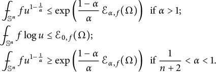 $$ \begin{align*} \frac{\ \ }{\ \ }{\hskip -0.4cm}\int_{\mathbb{S}^n}fu^{1-\frac1\alpha}&\leq \exp\left(\frac{1-\alpha}{\alpha}\,\mathcal{E}_{\alpha, f} (\Omega)\right) \mbox{ if}\ \alpha>1;\\ \frac{\ \ }{\ \ }{\hskip -0.4cm}\int_{\mathbb{S}^n}f\log u&\leq \mathcal{E}_{0, f} (\Omega);\\ \frac{\ \ }{\ \ }{\hskip -0.4cm}\int_{\mathbb{S}^n}fu^{1-\frac1\alpha}&\geq \exp\left(\frac{1-\alpha}{\alpha}\,\mathcal{E}_{\alpha, f} (\Omega)\right) \mbox{ if}\ \frac1{n+2}<\alpha<1. \end{align*} $$
Case 1:
 $\alpha>1$
.
$\alpha>1$
.
According to the condition in (i), we may choose
 $\zeta \in \{+1,-1\}$
such that
$\zeta \in \{+1,-1\}$
such that
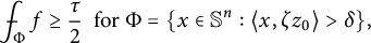 $$ \begin{align*}\frac{\ \ }{\ \ }{\hskip -0.4cm}\int_{\Phi}f\geq \frac{\tau}2 \mbox{ for }\Phi=\{x\in \mathbb{S}^n:\langle x,\zeta z_0\rangle>\delta\}, \end{align*} $$
and hence
 $\frac {R\zeta z_0}{n+1}\in \Omega $
by (2.2). Since
$\frac {R\zeta z_0}{n+1}\in \Omega $
by (2.2). Since
 $u_\sigma (x)\geq \langle \frac {R\zeta z_0}{n+1},x\rangle \geq \frac {R\delta }{n+1}$
for
$u_\sigma (x)\geq \langle \frac {R\zeta z_0}{n+1},x\rangle \geq \frac {R\delta }{n+1}$
for
 $x\in \Phi $
, we have
$x\in \Phi $
, we have
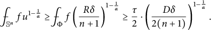 $$ \begin{align*}\frac{\ \ }{\ \ }{\hskip -0.4cm}\int_{\mathbb{S}^n}fu^{1-\frac1\alpha}\geq\frac{\ \ }{\ \ }{\hskip -0.4cm}\int_{\Phi}f\left(\frac{R\delta}{n+1}\right)^{1-\frac1\alpha}\geq \frac{\tau}2\cdot\left(\frac{D\delta}{2(n+1)}\right)^{1-\frac1\alpha}. \end{align*} $$
Case 2:
 $\alpha =1$
.
$\alpha =1$
.
To simplify notation, we consider the Borel probability measure
 $\mu (A)=\frac {\ \ }{\ \ }{\hskip -0.4cm}\int _Af$
on
$\mu (A)=\frac {\ \ }{\ \ }{\hskip -0.4cm}\int _Af$
on
 $S^n$
. Let
$S^n$
. Let
 $e_1,\ldots ,e_{n+1}\in \mathbb {S}^n$
be the principal directions associated with the ellipsoid E in (2.2), and let
$e_1,\ldots ,e_{n+1}\in \mathbb {S}^n$
be the principal directions associated with the ellipsoid E in (2.2), and let
 $r_1,\ldots ,r_{n+1}>0$
be the half axes of E with
$r_1,\ldots ,r_{n+1}>0$
be the half axes of E with
 $r_ie_i\in \partial E$
where we may assume that
$r_ie_i\in \partial E$
where we may assume that
 $r_1\leq \cdots \leq r_{n+1}$
. In particular, (2.2) yields that
$r_1\leq \cdots \leq r_{n+1}$
. In particular, (2.2) yields that
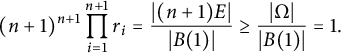 $$ \begin{align} (n+1)^{n+1}\prod_{i=1}^{n+1} r_i=\frac{|(n+1)E|}{|B(1)|}\geq \frac{|\Omega|}{|B(1)|}=1. \end{align} $$
We observe that for any
 $v\in \mathbb {S}^n$
, there exists
$v\in \mathbb {S}^n$
, there exists
 $e_i$
such that
$e_i$
such that
 $|\langle v,e_i\rangle |\geq \frac {1}{\sqrt {n+1}}> \frac {\delta }{n+1}$
. For
$|\langle v,e_i\rangle |\geq \frac {1}{\sqrt {n+1}}> \frac {\delta }{n+1}$
. For
 $i=1,\ldots ,n+1$
, we define
$i=1,\ldots ,n+1$
, we define
 $$ \begin{align*}B_i=\left\{v\in \mathbb{S}^n:|\langle v,e_i\rangle|\geq \frac{\delta}{n+1}\mbox{ and } |\langle v,e_j\rangle|<\frac{\delta}{n+1}\mbox{ for }j>i\right\}. \end{align*} $$
In particular,
 $B_i\subset \Psi (L_i\cap \mathbb {S}^n,\delta )$
for
$B_i\subset \Psi (L_i\cap \mathbb {S}^n,\delta )$
for
 $i=1,\ldots ,n$
and
$i=1,\ldots ,n$
and
 $L_i=\mathrm {lin}\{e_1,\ldots ,e_i\}$
.
$L_i=\mathrm {lin}\{e_1,\ldots ,e_i\}$
.
It follows that
 $\mathbb {S}^n$
is partitioned into the Borel sets
$\mathbb {S}^n$
is partitioned into the Borel sets
 $B_1,\ldots ,B_{n+1}$
, and as
$B_1,\ldots ,B_{n+1}$
, and as
 $B_i\subset \Psi (L_i\cap \mathbb {S}^n,\delta )$
for
$B_i\subset \Psi (L_i\cap \mathbb {S}^n,\delta )$
for
 $i=1,\ldots ,n$
, we have
$i=1,\ldots ,n$
, we have
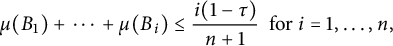 $$ \begin{align} \mu(B_1)+\cdots+\mu(B_i)&\leq \frac{i(1-\tau)}{n+1} \mbox{ for}\ i=1,\ldots,n, \end{align} $$
 $$ \begin{align} \mu(B_1)+\cdots+\mu(B_{n+1})&= 1. \end{align} $$
For
 $\zeta =\frac {1-\tau }{n+1}$
, we have
$\zeta =\frac {1-\tau }{n+1}$
, we have
 $0< \zeta <\frac 1{n+1}$
, and define
$0< \zeta <\frac 1{n+1}$
, and define
 $$ \begin{align} \beta_i&= \mu(B_i)-\zeta\mbox{ for}\ i=1,\ldots,n, \end{align} $$
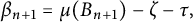 $$ \begin{align} \beta_{n+1}&= \mu(B_{n+1})-\zeta-\tau, \end{align} $$
 $$ \begin{align} \beta_1+\cdots+\beta_i&\leq 0\mbox{ for}\ i=1,\ldots,m-1, \end{align} $$
 $$ \begin{align} \beta_1+\cdots+\beta_{n+1}&= 0. \end{align} $$
As
 $r_ie_i\in \Omega $
, it follows from the definition of
$r_ie_i\in \Omega $
, it follows from the definition of
 $B_i$
that
$B_i$
that
 $u(x)\geq \langle x,r_ie_i\rangle \geq r_i\cdot \frac {\delta }{n+1}$
for
$u(x)\geq \langle x,r_ie_i\rangle \geq r_i\cdot \frac {\delta }{n+1}$
for
 $x\in B_i$
,
$x\in B_i$
,
 $i=1,\ldots ,n+1$
. We deduce from applying (2.3), (2.5)–(2.9),
$i=1,\ldots ,n+1$
. We deduce from applying (2.3), (2.5)–(2.9),
 $r_1\leq \cdots \leq r_{n+1}$
, and
$r_1\leq \cdots \leq r_{n+1}$
, and
 $\zeta <\frac 1{n+1}$
that
$\zeta <\frac 1{n+1}$
that
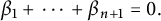
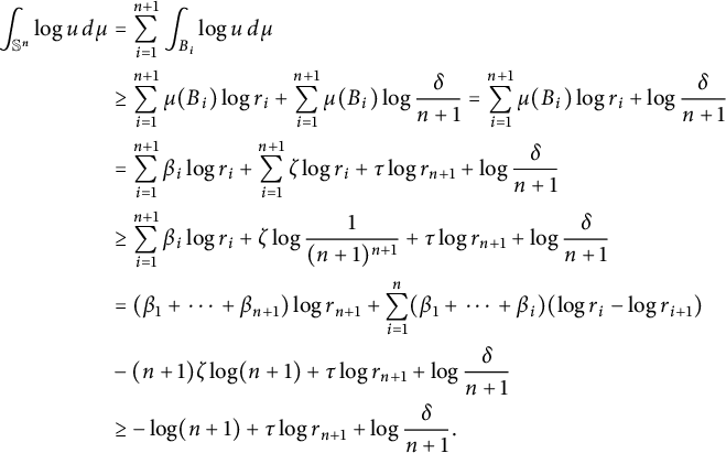 $$ \begin{align*} \int_{\mathbb{S}^n}\log u\,d\mu&= \sum_{i=1}^{n+1}\int_{B_i}\log u\,d\mu\\ &\geq \sum_{i=1}^{n+1}\mu(B_i)\log r_i+\sum_{i=1}^{n+1}\mu(B_i)\log \frac{\delta}{n+1} = \sum_{i=1}^{n+1}\mu(B_i)\log r_i+\log \frac{\delta}{n+1}\\ &= \sum_{i=1}^{n+1}\beta_i\log r_i+\sum_{i=1}^{n+1}\zeta \log r_i +\tau\log r_{n+1}+\log \frac{\delta}{n+1}\\ &\geq \sum_{i=1}^{n+1}\beta_i\log r_i+\zeta\log \frac{1}{(n+1)^{n+1}} +\tau\log r_{n+1}+\log \frac{\delta}{n+1}\\ &= (\beta_1+\cdots+\beta_{n+1})\log r_{n+1}+ \sum_{i=1}^{n}(\beta_1+\cdots+\beta_i)(\log r_i-\log r_{i+1})\\ & -(n+1)\zeta\log (n+1) +\tau\log r_{n+1}+\log \frac{\delta}{n+1}\\ &\geq -\log (n+1)+\tau\log r_{n+1}+\log \frac{\delta}{n+1}. \end{align*} $$
Now,
 $D\leq (n+1)\mathrm {diam}\,E=2(n+1)r_{n+1}\leq (n+1)^2r_{n+1}$
and
$D\leq (n+1)\mathrm {diam}\,E=2(n+1)r_{n+1}\leq (n+1)^2r_{n+1}$
and
 $\tau <1$
, and hence
$\tau <1$
, and hence
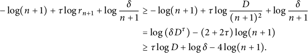 $$ \begin{align*} -\log (n+1)+\tau\log r_{n+1}+\log \frac{\delta}{n+1}&\geq -\log (n+1)+\tau\log \frac{D}{(n+1)^2} +\log \frac{\delta}{n+1}\\ &= \log\left(\delta D^\tau\right)-(2+2\tau)\log (n+1)\\ &\geq \tau\log D +\log\delta-4\log(n+1). \end{align*} $$
In particular, we conclude that
 $$ \begin{align*}\mathcal{E}_{1, f} (\Omega)\geq \frac{\ \ }{\ \ }{\hskip -0.4cm}\int_{\mathbb{S}^n}f\log u =\int_{\mathbb{S}^n}\log u\,d\mu \geq\tau\log D +\log\delta-4\log(n+1). \end{align*} $$
Case 3:
 $\frac 1{n+2}<\alpha <1$
.
$\frac 1{n+2}<\alpha <1$
.
In this case,
 $-(n+1)<1-\frac 1\alpha <0$
. We may assume that
$-(n+1)<1-\frac 1\alpha <0$
. We may assume that
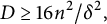 $$ \begin{align*}D\geq 16n^2/\delta^2, \end{align*} $$
and we consider
 $$ \begin{align*} \Phi_0&= \left\{x\in \mathbb{S}^n:\,u(x)> \sqrt{2R}\right\},\\ \Phi_1&= \left\{x\in \mathbb{S}^n:\,u(x)\leq \sqrt{2R}\right\}. \end{align*} $$
Concerning
 $\Phi _0$
, we have
$\Phi _0$
, we have
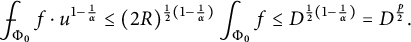 $$ \begin{align} \frac{\ \ }{\ \ }{\hskip -0.4cm}\int_{\Phi_0}f\cdot u^{1-\frac1\alpha}\leq (2R)^{\frac12(1-\frac1\alpha)}\int_{\Phi_0}f\leq D^{\frac12(1-\frac1\alpha)}=D^{\frac{p}2}. \end{align} $$
On the other hand, we have
 $\pm \frac {R}{(n+1)}\,z_0\in \Omega $
by (2.2), thus any
$\pm \frac {R}{(n+1)}\,z_0\in \Omega $
by (2.2), thus any
 $x\in \Phi _1$
satisfies
$x\in \Phi _1$
satisfies
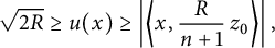 $$ \begin{align*}\sqrt{2R}\geq u(x)\geq \left|\left\langle x,\frac{R}{n+1}\,z_0\right\rangle\right|, \end{align*} $$
and hence
 $|\langle x,z_0\rangle |\leq (n+1)\sqrt {\frac {2}{R}}\leq \frac {4n}{\sqrt {D}}\leq \delta $
; or in other words,
$|\langle x,z_0\rangle |\leq (n+1)\sqrt {\frac {2}{R}}\leq \frac {4n}{\sqrt {D}}\leq \delta $
; or in other words,
 $$ \begin{align*}\Phi_1\subset \Psi(z_{0}^\bot\cap \mathbb{S}^n,\delta). \end{align*} $$
It follows from
 $|\Omega |=|B(1)|$
and the Blaschke–Santaló inequality (cf. [Reference Schneider45]) that
$|\Omega |=|B(1)|$
and the Blaschke–Santaló inequality (cf. [Reference Schneider45]) that
 $$ \begin{align*}\int_{\mathbb{S}^n} u^{-(n+1)}\leq (n+1)|B(1)|=\omega_{n},\mbox{ and hence } \frac{\ \ }{\ \ }{\hskip -0.4cm}\int_{\mathbb{S}^n} u^{-(n+1)}\leq 1. \end{align*} $$
For
 $p=1-\frac 1\alpha \in (-n-1,0)$
, Hölder’s inequality and
$p=1-\frac 1\alpha \in (-n-1,0)$
, Hölder’s inequality and
 $\int _{\Phi _1}f^{\frac {n+1}{n+1+p}}< \tau ^{\frac {n+1}{n+1+p}}$
yield
$\int _{\Phi _1}f^{\frac {n+1}{n+1+p}}< \tau ^{\frac {n+1}{n+1+p}}$
yield
 $$ \begin{align*}\frac{\ \ }{\ \ }{\hskip -0.4cm}\int_{\Phi_1}f\cdot u^{1-\frac1\alpha}\leq \left(\frac{\ \ }{\ \ }{\hskip -0.4cm}\int_{\Phi_1}f^{\frac{n+1}{n+1+p}}\right)^{\frac{n+1+p}{n+1}} \left(\frac{\ \ }{\ \ }{\hskip -0.4cm}\int_{\Phi_1} u_\sigma^{-(n+1)}\right)^{\frac{|p|}{n+1}}\leq \left(\frac{\ \ }{\ \ }{\hskip -0.4cm}\int_{\Phi_1}f^{\frac{n+1}{n+1+p}}\right)^{\frac{n+1+p}{n+1}}\leq \tau. \end{align*} $$
Finally, adding the last estimate to (2.10) yields
 $$ \begin{align*}\exp\left(\frac{\alpha-1}{\alpha}\,\mathcal{E}_{\alpha, f} (\Omega)\right)\leq \frac{\ \ }{\ \ }{\hskip -0.4cm}\int_{\mathbb{S}^n}f\cdot u^{1-\frac1\alpha}\leq D^{\frac{p}2}+\tau, \end{align*} $$
and hence the conditions either
 $\tau \leq \frac 12\frac {\ \ }{\ \ }{\hskip -0.4cm}\int _{\mathbb {S}^n}f\cdot u^{1-\frac 1\alpha }$
or
$\tau \leq \frac 12\frac {\ \ }{\ \ }{\hskip -0.4cm}\int _{\mathbb {S}^n}f\cdot u^{1-\frac 1\alpha }$
or
 $\tau \leq \frac 12\exp \left (\frac {1-\alpha }{\alpha }\,\mathcal {E}_{\alpha , f} (\Omega )\right )$
on
$\tau \leq \frac 12\exp \left (\frac {1-\alpha }{\alpha }\,\mathcal {E}_{\alpha , f} (\Omega )\right )$
on
 $\tau $
implies (iii).
$\tau $
implies (iii).
3 Anisotropic flows and monotonicity of entropies
The following theorem was proved by Andrews in [Reference Andrews4] (see also for a discussion of contracting of non-homogeneous fully nonlinear anisotropic curvature flows in [Reference Guan, Huang and Liu24]).
Theorem 3.1 [Reference Andrews4]
For any
 $\alpha>0$
and positive
$\alpha>0$
and positive
 $f\in C^{\infty }(\mathbb S^n)$
and any initial smooth, strictly convex hypersurface
$f\in C^{\infty }(\mathbb S^n)$
and any initial smooth, strictly convex hypersurface
 $\tilde M_0\subset \mathbb R^{n+1}$
, the hypersurfaces
$\tilde M_0\subset \mathbb R^{n+1}$
, the hypersurfaces
 $\tilde M_{\tau }$
given by the solution of (1.7) exist for a finite time T and converge in Hausdorff distance to a point
$\tilde M_{\tau }$
given by the solution of (1.7) exist for a finite time T and converge in Hausdorff distance to a point
 $p \in \mathbb R^{n+1}$
as
$p \in \mathbb R^{n+1}$
as
 $\tau $
approaches T.
$\tau $
approaches T.
Assuming
 $$\begin{align*}\frac{\ \ }{\ \ }{\hskip -0.4cm}\int_{\mathbb S^n}f=1, \quad |\Omega_0|=|B(1)|,\end{align*}$$
solution (1.7) yields a smooth convex solution to the normalized flow (1.8) with volume preserved.
Set
 $$ \begin{align} h_z(x,t)\doteqdot f(x) u_z^{-\frac{1}{\alpha}}(x,t)K(x,t), \quad d\sigma_t(x) =\frac{u_z(x,t)}{K(x,t)}d\theta(x).\end{align} $$
Note that
 $\frac {\ \ }{\ \ }{\hskip -0.4cm}\int _{\mathbb {S}^n} d\sigma _t(x) =\frac {\ \ }{\ \ }{\hskip -0.4cm}\int _{\mathbb {S}^n} d\theta (x) =1$
.
$\frac {\ \ }{\ \ }{\hskip -0.4cm}\int _{\mathbb {S}^n} d\sigma _t(x) =\frac {\ \ }{\ \ }{\hskip -0.4cm}\int _{\mathbb {S}^n} d\theta (x) =1$
.
Since the un-normalized flow (1.7) shrinks to a point in finite time, we may assume that it is the origin. Then the support function
 $u(x,t)$
is positive for the normalized flow (1.8).
$u(x,t)$
is positive for the normalized flow (1.8).
Lemma 3.2
-
(a) The entropy
$ \mathcal {E}_{\alpha , f}(\Omega _{t})$
defined in (1.5) is monotonically decreasing, (3.2)
$$ \begin{align} \mathcal{E}_{\alpha, f}(\Omega_{t_2})\le \mathcal{E}_{\alpha, f}(\Omega_{t_1}), \quad \forall t_1\le t_2 \in [0, \infty).\end{align} $$
-
(b) There is
$D>0$
depending only on
$\inf f, \sup f, \alpha , \Omega _0$
such that (3.3)
$$ \begin{align} \mathrm{diam}\,\Omega_t=D(t)\le D, \ \forall t\ge 0.\end{align} $$
-
(c)
$\forall t_0\in [0, \infty )$
, (3.4)
$$ \begin{align} \mathcal{E}_{\alpha, f}(\Omega_{t_0}, 0)\ge \mathcal{E}_{\alpha, f, \infty} +\int_{t_0}^{\infty}\left(\frac{\frac{\ \ }{\ \ }{\hskip -0.4cm}\int_{\mathbb{S}^n} h^{\alpha+1}(x,t)\, d\sigma_t} {\frac{\ \ }{\ \ }{\hskip -0.4cm}\int_{\mathbb{S}^n} h(x,t) \, d\sigma_t \cdot \frac{\ \ }{\ \ }{\hskip -0.4cm}\int_{\mathbb{S}^n} h^{\alpha}(x,t)\, d\sigma_t}-1\right)\, dt,\end{align} $$
where
$$\begin{align*}h(x,t)=h_0(x, t), \ \mathcal{E}_{\alpha, f, \infty}\doteqdot\lim_{t\to \infty} \mathcal{E}_{\alpha, f}(\Omega_{t}).\end{align*}$$


Proof
-
(a) We follow argument in [Reference Guan and Ni26]. For each
$T_0>$
fixed, pick
$T> T_0$
. Let
$a^{T}=(a^{T}_1,\ldots , a^{T}_{n+1})$
be an interior point of
$\Omega _T$
. Set
$u^T=u- e^{t-T}\sum _{i=1}^{n+1} a^T_ix_i$
; it satisfies equation (3.5)
$$ \begin{align} \frac{\partial}{\partial t}u^T(x, t)= -\frac{f^\alpha(x) K^{\alpha}(x, t)}{\frac{\ \ }{\ \ }{\hskip -0.4cm}\int_{\mathbb{S}^n}f^\alpha K^{\alpha-1}} +u^T(x,t).\end{align} $$
Note that since
$a^T$
is an interior point of
$\Omega _T$
and
$u(x,T)$
is the support function of
$\Omega _T$
with respect to
$a^T$
,
$u^T(x, T)> 0, \forall x\in \mathbb S^n$
. We claim Suppose
$$\begin{align*}u^T(x, t)>0, \ \forall t\in [0, T).\end{align*}$$
$u^T(x_0, t')\le 0$
for some
$0<t'<T, x_0\in \mathbb S^n$
, and equation (3.5) implies
$u^T(x_0, t)<0$
for all
$t>t'$
, which contradicts to
$u^T(x, T)> 0$
.
Set
$a^T(t)=e^{t-T}a^T$
. By the claim,
$a^T(t)$
is in the interior of
$\Omega _t, \ \forall t\le T$
. Denote we rewrite equation (3.3) as
$$\begin{align*}d\sigma_{T,t}=u^T(x,t)K^{-1}(x,t)d\theta,\end{align*}$$
(3.6)We have
$$ \begin{align} \frac{\partial}{\partial t}u_{a^T(t)}(x,t)= -\frac{f^\alpha(x) K^{\alpha}(x, t)}{\frac{\ \ }{\ \ }{\hskip -0.4cm}\int_{\mathbb{S}^n}h_{a^T(t)}^{\alpha}(x,t)\, d\sigma_{T,t}} +u_{a^T(t)}(x,t).\end{align} $$
$$\begin{align*}\frac{\partial}{\partial t} \mathcal{E}_{\alpha, f}(\Omega_{t}, a^T(t))=\frac{-\frac{\ \ }{\ \ }{\hskip -0.4cm}\int_{\mathbb{S}^n} h_{a^T(t)}^{\alpha+1}(x,t)\, d\sigma_{T,t}} {\frac{\ \ }{\ \ }{\hskip -0.4cm}\int_{\mathbb{S}^n} h_{a^T(t)}(x,t) \, d\sigma_{T,t} \cdot \frac{\ \ }{\ \ }{\hskip -0.4cm}\int_{\mathbb{S}^n} h_{a^T(t)}^{\alpha}(x,t)\, d\sigma_{T,t}}+1.\end{align*}$$
Thus,
$\forall t<T$
, (3.7)Therefore,
$$ \begin{align} &\mathcal{E}_{\alpha, f}(\Omega_{t}, a^T(t))-\mathcal{E}_{\alpha, f}(\Omega_T, a^T)\\ \nonumber &= \int_{t}^{T}\frac{\ \ }{\ \ }{\hskip -0.4cm}\int_{\mathbb S^n} \left(\frac{\frac{\ \ }{\ \ }{\hskip -0.4cm}\int_{\mathbb{S}^n} h_{a^T(t)}^{\alpha+1}(x,t)\, d\sigma_{T,t}} {\frac{\ \ }{\ \ }{\hskip -0.4cm}\int_{\mathbb{S}^n} h_{a^T(t)}(x,t) \, d\sigma_{T,t} \cdot \frac{\ \ }{\ \ }{\hskip -0.4cm}\int_{\mathbb{S}^n} h_{a^T(t)}^{\alpha}(x,t)\, d\sigma_{T,t}}-1\right)\, dt\ge 0. \end{align} $$
Since
$$\begin{align*}\mathcal{E}_{\alpha, f}(\Omega_{t})\ge\mathcal{E}_{\alpha, f}(\Omega_T, a^T), \ \forall t<T.\end{align*}$$
$a^T$
is arbitrary, (3.2) is proved.
-
(b) The boundedness of
$D(t)$
follows from Theorem 2.1 combined with the estimate
$\mathcal {E}_{\alpha , 1}(\Omega _{t})\leq \mathcal {E}_{\alpha , 1}(B(1))$
from (a) (see also [Reference Andrews, Guan and Ni6, Reference Guan and Ni26]). The only nontrivial case is when
$\frac 1{n+2}<\alpha <1$
because we have to choose a
$\tau $
independent of t. However, we may choose any
$\tau \in (0,1)$
with
$\tau \leq \frac 12\exp \left (\frac {1-\alpha }{\alpha }\,\mathcal {E}_{\alpha , f} (B(1))\right )$
according to
$\mathcal {E}_{\alpha , 1}(\Omega _{t})\leq \mathcal {E}_{\alpha , 1}(B(1))$
. -
(c)
$\forall \epsilon>0, \ \forall t_0$
fixed, pick
$T>T_0>t_0$
. As
$ \mathcal {E}_{\alpha , f}(\Omega _{T})$
is bounded by (a),
$\exists a^T$
inside
$\Omega _T$
such that
$ \mathcal {E}_{\alpha , f}(\Omega _{T})\le \mathcal {E}_{\alpha , f}(\Omega _{T}, a^T)+\epsilon $
. By (3.7),
$$ \begin{align*} &\mathcal{E}_{\alpha, f}(\Omega_{t_0}, a^T(t_0))-\mathcal{E}_{\alpha, f}(\Omega_{T})\\ &\ge \int_{t_0}^{T_0}\frac{\ \ }{\ \ }{\hskip -0.4cm}\int_{\mathbb S^n} \left(\frac{\frac{\ \ }{\ \ }{\hskip -0.4cm}\int_{\mathbb{S}^n} h_{a^T(t)}^{\alpha+1}(x,t)\, d\sigma_{T,t}} {\frac{\ \ }{\ \ }{\hskip -0.4cm}\int_{\mathbb{S}^n} h_{a^T(t)}(x,t) \, d\sigma_{T,t} \cdot \frac{\ \ }{\ \ }{\hskip -0.4cm}\int_{\mathbb{S}^n} h_{a^T(t)}^{\alpha}(x,t)\, d\sigma_{T,t}}-1\right)\, dt-\epsilon. \end{align*} $$
As
$|a^T|\le D, \ \forall T$
, let
$T\to \infty $
,
$$\begin{align*}a^T(t)\to 0, \ u^T(x,t)\to u(x,t), \ \ \mbox{ uniformly for}\ 0\le t\le T_0, x\in \mathbb S^n. \end{align*}$$
We obtain
$\forall t_0<T_0$
,
$$ \begin{align*} \mathcal{E}_{\alpha, f}(\Omega_{t_0}, 0)-\mathcal{E}_{\alpha, f, \infty}\ge \int_{t_0}^{T_0}\frac{\ \ }{\ \ }{\hskip -0.4cm}\int_{\mathbb S^n} \left(\frac{\frac{\ \ }{\ \ }{\hskip -0.4cm}\int_{\mathbb{S}^n} h^{\alpha+1}(x,t)\, d\sigma_t} {\frac{\ \ }{\ \ }{\hskip -0.4cm}\int_{\mathbb{S}^n} h(x,t) \, d\sigma_t \cdot \frac{\ \ }{\ \ }{\hskip -0.4cm}\int_{\mathbb{S}^n} h^{\alpha}(x,t)\, d\sigma_t}-1\right)\, dt-\epsilon.\end{align*} $$
Then let
$T_0\to \infty $
, as
$\epsilon>0$
is arbitrary, we obtain (3.4).


4 Weak convergence
The goal of this section is to prove the following statement.
Theorem 4.1 For a
 $C^\infty $
function
$C^\infty $
function
 $f:\mathbb {S}^n\to (0,\infty )$
and
$f:\mathbb {S}^n\to (0,\infty )$
and
 $\alpha>\frac 1{n+2}$
with
$\alpha>\frac 1{n+2}$
with
 $ \frac {\ \ }{\ \ }{\hskip -0.4cm}\int _{\mathbb {S}^n}f=1$
, there exist
$ \frac {\ \ }{\ \ }{\hskip -0.4cm}\int _{\mathbb {S}^n}f=1$
, there exist
 $\lambda>0$
and a convex body
$\lambda>0$
and a convex body
 $\Omega \subset \Bbb R^{n+1}$
with
$\Omega \subset \Bbb R^{n+1}$
with
 $o\in \Omega $
whose support function u is a (possibly weak) solution of the Monge–Ampère equation
$o\in \Omega $
whose support function u is a (possibly weak) solution of the Monge–Ampère equation
 $$ \begin{align} u^{\frac1\alpha}\det(\bar{\nabla}^2_{ij} u+u\bar{g}_{ij})= f \end{align} $$
and
 $\Omega $
satisfies that
$\Omega $
satisfies that
 $$ \begin{align} \mathcal{E}_{\alpha, f} (\lambda\Omega)\leq \mathcal{E}_{\alpha, f} (B(1)), \quad |\lambda\Omega|=|B(1)|, \end{align} $$
where
 $C^{-1}<\lambda <C$
for a
$C^{-1}<\lambda <C$
for a
 $C>1$
depending only on the
$C>1$
depending only on the
 $\alpha , \tau , \delta $
in Theorem 2.1 such that f satisfies the conditions in Theorem 2.1.
$\alpha , \tau , \delta $
in Theorem 2.1 such that f satisfies the conditions in Theorem 2.1.
From now on, we will assume that the f in Theorem 4.1 satisfies the corresponding condition in Theorem 2.1 and
 $\Omega _0=B(1)$
in (1.8). We note that for any
$\Omega _0=B(1)$
in (1.8). We note that for any
 $z\in B(1)$
,
$z\in B(1)$
,
 $v_z\leq 2$
for the support function
$v_z\leq 2$
for the support function
 $v_z$
of
$v_z$
of
 $B(1)$
at z, and hence if
$B(1)$
at z, and hence if
 $\alpha>\frac 1{n+2}$
, then
$\alpha>\frac 1{n+2}$
, then
 $$ \begin{align} \mathcal{E}_{\alpha, f_k} (B(1))\leq\left\{ \begin{array}{rl} \frac{\alpha}{\alpha-1}\cdot\log 2^{1-\frac1\alpha},&\mbox{ if }\alpha\neq 1,\\ \log 2,&\mbox{ if }\alpha=1. \end{array} \right. \end{align} $$
The following is a consequence of Theorem 2.1 and Lemma 3.2.
Lemma 4.2 There exist
 $C_{\alpha , \tau , \delta }>0, D_{\alpha , \tau , \delta }>0$
, and
$C_{\alpha , \tau , \delta }>0, D_{\alpha , \tau , \delta }>0$
, and
 $c_{\alpha , \tau , \delta }\in \mathbb R$
depending only on constants
$c_{\alpha , \tau , \delta }\in \mathbb R$
depending only on constants
 $\alpha , \tau , \delta $
in Theorem 2.1 such that, along (1.8), we have
$\alpha , \tau , \delta $
in Theorem 2.1 such that, along (1.8), we have
 $$ \begin{align} D(t)\le D_{\alpha, \tau, \delta},\ \mathcal{E}_{\alpha, f}(\Omega_{t}, 0)\ge c_{\alpha, \tau, \delta}, \ \frac{1}{C_{\alpha, \tau, \delta}}\le \frac{\ \ }{\ \ }{\hskip -0.4cm}\int_{\mathbb S^n} h(x,t)d\sigma_t\le C_{\alpha, \tau, \delta}.\end{align} $$
Proof For each
 $\alpha>\frac 1{n+2}$
fixed with condition on f as in Theorem 2.1,
$\alpha>\frac 1{n+2}$
fixed with condition on f as in Theorem 2.1,
 $\mathcal {E}_{\alpha , f}(\Omega _{t})$
is bounded from below in terms of the diameter
$\mathcal {E}_{\alpha , f}(\Omega _{t})$
is bounded from below in terms of the diameter
 $D(t)$
. Since
$D(t)$
. Since
 $|\Omega _t|=|B(1)|$
, we have
$|\Omega _t|=|B(1)|$
, we have
 $D(t)\ge 2$
by the Isodiametric Inequality (cf. [Reference Schneider45]). By Theorem 2.1,
$D(t)\ge 2$
by the Isodiametric Inequality (cf. [Reference Schneider45]). By Theorem 2.1,
 $\mathcal {E}_{\alpha , f}(\Omega _{t})$
is bounded from below by a constant
$\mathcal {E}_{\alpha , f}(\Omega _{t})$
is bounded from below by a constant
 $c_{\alpha , \tau , \delta }>0$
, and hence
$c_{\alpha , \tau , \delta }>0$
, and hence
 $\mathcal {E}_{\alpha , f, \infty } \ge c_{\alpha , \tau , \delta }$
. It follows from Lemma 3.2 that
$\mathcal {E}_{\alpha , f, \infty } \ge c_{\alpha , \tau , \delta }$
. It follows from Lemma 3.2 that
 $\mathcal {E}_{\alpha , f}(\Omega _{t})\le \mathcal {E}_{\alpha , f}(B(1))$
, and this estimate combined with (4.3) and Theorem 2.1 yields
$\mathcal {E}_{\alpha , f}(\Omega _{t})\le \mathcal {E}_{\alpha , f}(B(1))$
, and this estimate combined with (4.3) and Theorem 2.1 yields
 $D(t)\le D_{\alpha , \tau , \delta }$
where
$D(t)\le D_{\alpha , \tau , \delta }$
where
 $D_{\alpha , \tau , \delta }$
depends only on constants in condition on f in Theorem 2.1. Finally, the inequalities follow from Lemma 3.2.
$D_{\alpha , \tau , \delta }$
depends only on constants in condition on f in Theorem 2.1. Finally, the inequalities follow from Lemma 3.2.
Set
 $$ \begin{align} \eta(t)=\frac{\ \ }{\ \ }{\hskip -0.4cm}\int_{\mathbb{S}^n} h(x,t) \, d\sigma_{t}. \end{align} $$
We note that
 $\frac {\ \ }{\ \ }{\hskip -0.4cm}\int _{\mathbb {S}^n} h(x,t) \, d\sigma _{t} $
is monotone and bounded from below and above by Lemma 4.2, and hence we have
$\frac {\ \ }{\ \ }{\hskip -0.4cm}\int _{\mathbb {S}^n} h(x,t) \, d\sigma _{t} $
is monotone and bounded from below and above by Lemma 4.2, and hence we have
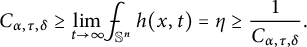 $$ \begin{align}C_{\alpha, \tau, \delta}\ge \lim_{t\to \infty} \frac{\ \ }{\ \ }{\hskip -0.4cm}\int_{\mathbb{S}^n} h(x,t)=\eta\ge \frac1{C_{\alpha, \tau, \delta}}.\end{align} $$
By Lemma 3.2 and Corollary 4.2,
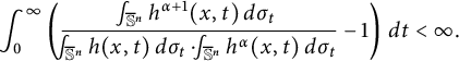 $$ \begin{align} \int_0^{\infty} \left(\frac{\frac{\ \ }{\ \ }{\hskip -0.4cm}\int_{\mathbb{S}^n} h^{\alpha+1}(x,t)\, d\sigma_t} {\frac{\ \ }{\ \ }{\hskip -0.4cm}\int_{\mathbb{S}^n} h(x,t) \, d\sigma_t \cdot \frac{\ \ }{\ \ }{\hskip -0.4cm}\int_{\mathbb{S}^n} h^{\alpha}(x,t)\, d\sigma_t}-1\right)\, dt<\infty.\end{align} $$
Since the integrand is nonnegative,
 $\exists t_k\to \infty $
such that
$\exists t_k\to \infty $
such that
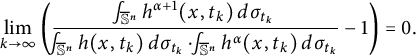 $$ \begin{align} \lim_{k\to \infty} \left( \frac{\frac{\ \ }{\ \ }{\hskip -0.4cm}\int_{\mathbb{S}^n}h^{\alpha+1}(x,t_k)\, d\sigma_{t_k}} {\frac{\ \ }{\ \ }{\hskip -0.4cm}\int_{\mathbb{S}^n} h(x,t_k) \, d\sigma_{t_k} \cdot \frac{\ \ }{\ \ }{\hskip -0.4cm}\int_{\mathbb{S}^n} h^{\alpha}(x,t_k)\, d\sigma_{t_k}}-1\right)=0.\end{align} $$
This implies
 $$ \begin{align} \lim_{k\to \infty}\frac{\left(\frac{\ \ }{\ \ }{\hskip -0.4cm}\int_{\mathbb{S}^n}h^{\alpha+1}(x,t_k)\, d\sigma_{t_k}\right)^{\frac{1}{1+\alpha}}}{\frac{\ \ }{\ \ }{\hskip -0.4cm}\int_{\mathbb{S}^n} h(x,t_k) \, d\sigma_{t_k} }= \lim_{k\to \infty}\frac{\left(\frac{\ \ }{\ \ }{\hskip -0.4cm}\int_{\mathbb{S}^n}h^{\alpha+1}(x,t_k)\, d\sigma_{t_k}\right)^{\frac{\alpha}{1+\alpha}}}{\frac{\ \ }{\ \ }{\hskip -0.4cm}\int_{\mathbb{S}^n} h^{\alpha}(x,t_k)\, d\sigma_{t_k}}= 1.\end{align} $$
After considering a subsequence, we may assume that
 $$ \begin{align} \Omega_{t_k}\to \Omega, \quad u(x,t_k)\to u(x),\end{align} $$
where u is the support function of
 $\Omega $
. In view of (4.9) and (4.6),
$\Omega $
. In view of (4.9) and (4.6),
 $$ \begin{align} \lim_{k\to \infty} \frac{\ \ }{\ \ }{\hskip -0.4cm}\int_{\mathbb{S}^n}h^{\alpha+1}(x,t_k)\, d\sigma_{t_k}=\eta^{1+\alpha},\ \lim_{k\to \infty}\frac{\ \ }{\ \ }{\hskip -0.4cm}\int_{\mathbb{S}^n} h^{\alpha}(x,t_k)\, d\sigma_{t_k}= \eta^{\alpha}.\end{align} $$
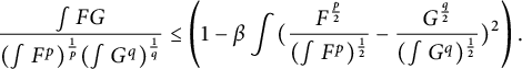
The following lemma is crucial for the weak convergence, which is a refined form of the classical Hölder inequality.Footnote 1
Lemma 4.3 Let
 $p,\ q\in \mathbb R^+$
with
$p,\ q\in \mathbb R^+$
with
 $\frac 1p+\frac 1q=1$
, and set
$\frac 1p+\frac 1q=1$
, and set
 $\beta =\min \{\frac 1p, \frac 1q\}$
. Let
$\beta =\min \{\frac 1p, \frac 1q\}$
. Let
 $(M,\mu )$
be a measurable space;
$(M,\mu )$
be a measurable space;
 $\forall F\in L^p, \ G\in L^q$
,
$\forall F\in L^p, \ G\in L^q$
,
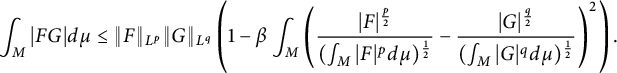 $$ \begin{align} \int_M |FG| d\mu \le \|F\|_{L^p}\|G\|_{L^q}\left(1-\beta\int_M \left(\frac{|F|^{\frac{p}2}}{(\int_M |F|^p d\mu)^{\frac12}}-\frac{|G|^{\frac{q}2}}{(\int_M |G|^qd\mu )^{\frac12}}\right)^2\right).\end{align} $$
Proof We first prove the following Claim.
 $\forall s, t\in \mathbb R$
,
$\forall s, t\in \mathbb R$
,
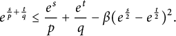 $$ \begin{align} e^{\frac{s}{p}+\frac{t}{q}}\le \frac{e^s}{p}+\frac{e^t}{q}-\beta(e^{\frac{s}2}-e^{\frac{t}2})^2.\end{align} $$
We may assume
 $t\ge s$
, set
$t\ge s$
, set
 $\tau =t-s$
, and (4.13) is equivalent to
$\tau =t-s$
, and (4.13) is equivalent to
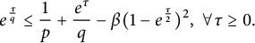 $$ \begin{align} e^{\frac{\tau}{q}}\le \frac{1}{p}+\frac{e^{\tau}}{q}-\beta(1-e^{\frac{\tau}2})^2, \ \forall \tau\ge 0.\end{align} $$
Set
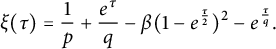 $$\begin{align*}\xi(\tau)=\frac{1}{p}+\frac{e^{\tau}}{q}-\beta(1-e^{\frac{\tau}2})^2-e^{\frac{\tau}{q}}.\end{align*}$$
We have
 $\xi (0)=0$
,
$\xi (0)=0$
,
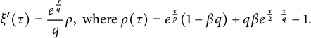 $$\begin{align*}\xi'(\tau)=\frac{e^{\frac{\tau}q}}{q}\rho, \ \mbox{where} \ \rho(\tau)=e^{\frac{\tau}{p}}(1-\beta q)+q\beta e^{\frac{\tau}2-\frac{\tau}q}-1.\end{align*}$$
If
 $\beta =\frac 1q$
, then
$\beta =\frac 1q$
, then
 $\frac 1q\le \frac 12$
; since
$\frac 1q\le \frac 12$
; since
 $\tau \ge 0$
,
$\tau \ge 0$
,
 $$\begin{align*}\rho(\tau)=e^{\frac{\tau}{p}}(1-\beta q)+q\beta e^{\frac{\tau}2-\frac{\tau}q}-1=e^{\frac{\tau}2-\frac{\tau}q}-1\ge 0.\end{align*}$$
If
 $\beta =\frac 1p$
, then
$\beta =\frac 1p$
, then
 $\frac 1q\ge \frac 12$
; we have
$\frac 1q\ge \frac 12$
; we have
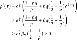 $$ \begin{align*} \rho'(\tau)&=e^{\frac{\tau}{p}}\left(\frac{1-\beta q}p+\beta q(\frac12-\frac1q)e^{\frac{\tau}2-\frac{\tau}q}\right)\\ & \ge e^{\frac{\tau}{p}}\left(\frac{1-\beta q}p+\beta q(\frac12-\frac1q)\right)\\ &\ge e^{\frac{\tau}{p}}\beta q(\frac12-\frac1p)\ge 0.\end{align*} $$
We conclude that
 $$\begin{align*}\rho(\tau)\ge 0, \ \forall \tau\ge 0.\end{align*}$$
In turn,
 $$\begin{align*}\xi'(\tau)\ge 0, \ \forall \tau\ge o.\end{align*}$$
This yields (4.14) and (4.13). The Claim is verified.
Back to the proof of the lemma. We may assume
 $$\begin{align*}F\ge 0, \ g\ge 0, \ \int F^p>0, \ \int G^q>0.\end{align*}$$
Set
 $$\begin{align*}e^s=\frac{F^p}{\int F^p}, \quad e^t=\frac{G^q}{\int G^q}.\end{align*}$$
Put them into (4.13) and integrate, as
 $\frac 1p+\frac 1q=1$
,
$\frac 1p+\frac 1q=1$
,
 $$\begin{align*}\frac{\int FG}{(\int F^p)^{\frac1{p}}(\int G^q)^{\frac1{q}}}\le \left(1-\beta\int (\frac{F^{\frac{p}2}}{(\int F^p)^{\frac12}}-\frac{G^{\frac{q}2}}{(\int G^q)^{\frac12}})^2\right).\\[-34pt] \end{align*}$$
We prove weak convergence.
Proposition 4.4
 $\forall \alpha>\frac {1}{n+2}$
, suppose that (4.10) and (4.11) hold. Denote
$\forall \alpha>\frac {1}{n+2}$
, suppose that (4.10) and (4.11) hold. Denote
 $$\begin{align*}u_{k}=u(x, t_k), \ \sigma_{n,k}=\sigma_n(u_{ij}(x,t_k)+u(x,t_k)\delta_{ij}).\end{align*}$$
Then
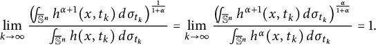
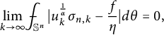 $$ \begin{align} \lim_{k\to \infty} \frac{\ \ }{\ \ }{\hskip -0.4cm}\int_{\mathbb S^n} |u_k^{\frac{1}\alpha}\sigma_{n,k}-\frac{f}{\eta}| d\theta =0,\end{align} $$
where
 $\eta $
is defined in (4.5) which is bounded from below and above in (4.6). As a consequence, there is a convex body
$\eta $
is defined in (4.5) which is bounded from below and above in (4.6). As a consequence, there is a convex body
 $\Omega \subset \mathbb R^{n+1}$
with
$\Omega \subset \mathbb R^{n+1}$
with
 $o\in \Omega $
,
$o\in \Omega $
,
 $$\begin{align*}|\Omega|=|B(1)|, \quad \mathcal{E}_{\alpha, f}(\Omega_{t})\le \mathcal{E}_{\alpha, f}(B(1)),\end{align*}$$
and its support function u satisfies
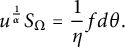 $$ \begin{align} u^{\frac1{\alpha}} S_{\Omega}=\frac1{\eta} fd \theta. \end{align} $$
Proof We only need to verify (4.15). By (4.11), it is equivalent to prove
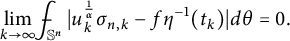 $$ \begin{align} \lim_{k\to \infty} \frac{\ \ }{\ \ }{\hskip -0.4cm}\int_{\mathbb S^n} |u_k^{\frac{1}\alpha}\sigma_{n,k}-f\eta^{-1}(t_k)| d\theta =0.\end{align} $$
Since
 $D(t_k)$
is bounded,
$D(t_k)$
is bounded,
 $$\begin{align*}\frac{\ \ }{\ \ }{\hskip -0.4cm}\int_{\mathbb S^n} u_k^{\frac{1}{\alpha^2}}\sigma_{n,k} d\theta\le (D(t_k))^{\frac1{\alpha^2}}\frac{\ \ }{\ \ }{\hskip -0.4cm}\int_{\mathbb S^n} u_k^{\frac{1}{\alpha^2}}\sigma_{n,k} d\theta\le (D(t_k))^{\frac1{\alpha^2}}|\partial \Omega_{t_k}|\le C.\end{align*}$$
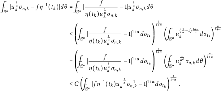 $$ \begin{align} \frac{\ \ }{\ \ }{\hskip -0.4cm}\int_{\mathbb S^n} |u_k^{\frac{1}\alpha}\sigma_{n,k}-f\eta^{-1}(t_k)| d\theta &=\frac{\ \ }{\ \ }{\hskip -0.4cm}\int_{\mathbb S^n} |\frac{f}{\eta(t_k)u_k^{\frac{1}\alpha}\sigma_{n,k}}-1 |u_k^{\frac{1}\alpha}\sigma_{n,k} d\theta\nonumber\\ &\le \left(\frac{\ \ }{\ \ }{\hskip -0.4cm}\int_{\mathbb S^n} |\frac{f}{\eta(t_k)u_k^{\frac{1}\alpha}\sigma_{n,k}}-1 |^{1+\alpha} d\sigma_{t_k}\right)^{\frac{1}{1+\alpha}}\left(\frac{\ \ }{\ \ }{\hskip -0.4cm}\int_{\mathbb S^n} u_k^{(\frac1{\alpha}-1)\frac{1+\alpha}{\alpha}}d\sigma_{t_k}\right)^{\frac{\alpha}{1+\alpha}}\nonumber \\ &= \left(\frac{\ \ }{\ \ }{\hskip -0.4cm}\int_{\mathbb S^n} |\frac{f}{\eta(t_k)u_k^{\frac{1}\alpha}\sigma_{n,k}}-1 |^{1+\alpha} d\sigma_{t_k}\right)^{\frac{1}{1+\alpha}}\left(\frac{\ \ }{\ \ }{\hskip -0.4cm}\int_{\mathbb S^n} u_k^{\frac{1}{\alpha^2}}\sigma_{n,k} d\theta\right)^{\frac{\alpha}{1+\alpha}}\nonumber \\ &\le C \left(\frac{\ \ }{\ \ }{\hskip -0.4cm}\int_{\mathbb S^n} |f\eta^{-1}(t_k)u_k^{-\frac{1}\alpha}\sigma^{-1}_{n,k}-1 |^{1+\alpha} d\sigma_{t_k}\right)^{\frac{1}{1+\alpha}}. \end{align} $$
By (4.8), (4.11), and Lemma 4.3, with
 $p=\alpha +1$
,
$p=\alpha +1$
,
 $F^{\frac {1}{1+\alpha }}=h(x,t_k)$
,
$F^{\frac {1}{1+\alpha }}=h(x,t_k)$
,
 $G=1$
,
$G=1$
,
 $$ \begin{align} \lim_{k\to \infty} \frac{\ \ }{\ \ }{\hskip -0.4cm}\int \left((\frac{h(x,t_k)}{\eta(t_k)})^{\frac{1+\alpha}2}-1\right)^2d\sigma_{t_k}=0.\end{align} $$
For
 $t_k$
fixed, let
$t_k$
fixed, let
 $$\begin{align*}\gamma_k(x)=f\eta^{-1}(t_k)u_k^{-\frac{1}\alpha}\sigma^{-1}_{n,k}=h(x,t_k)\eta^{-1}(t_k)\end{align*}$$
and set
 $$\begin{align*}\Sigma_{k}=\left\{x\in \mathbb S^n \ | \ |\gamma_k(x)-1|\le \frac12\right\}.\end{align*}$$
It is straightforward to check that
 $\exists A_{\alpha }\ge 1$
depending only on
$\exists A_{\alpha }\ge 1$
depending only on
 $\alpha $
such that
$\alpha $
such that
 $$ \begin{align*} A_{\alpha}|\gamma^{\frac{1+\alpha}2}_k(x)-1|&\ge |\gamma_k(x)-1|, \ \forall x\in \Sigma_k, \\ A_{\alpha} |\gamma^{\frac{1+\alpha}2}_k(x)-1|^{2}&\ge |\gamma_k(x)-1|^{1+\alpha}, \ \forall x\in \Sigma_{k}^c.\end{align*} $$
Since
 $ |\gamma ^{\frac {1+\alpha }2}_k(x)-1|\le 2^{1+\alpha }, \ \forall x\in \Sigma _k$
, let
$ |\gamma ^{\frac {1+\alpha }2}_k(x)-1|\le 2^{1+\alpha }, \ \forall x\in \Sigma _k$
, let
 $\delta =\min \{1+\alpha , 2\}$
,
$\delta =\min \{1+\alpha , 2\}$
,
 $$ \begin{align*} \ \frac{\ \ }{\ \ }{\hskip -0.4cm}\int_{\mathbb S^n} |\gamma_k(x)-1 |^{1+\alpha} d\sigma_{t_k}=&\frac{1}{\omega_n}\left(\int_{\Sigma_k} |\gamma_k(x)-1 |^{1+\alpha} d\sigma_{t_k}+\int_{\Sigma_k^c} |\gamma_k(x)-1 |^{1+\alpha} d\sigma_{t_k}\right)\\ \le & \frac{A^{1+\alpha}_{\alpha}}{\omega_n} \left(\int_{\Sigma_k} |\gamma_k^{\frac{1+\alpha}2}(x)-1 |^{1+\alpha} d\sigma_{t_k}+\int_{\Sigma_k^c} |\gamma_k^{\frac{1+\alpha}2}(x)-1 |^{2} d\sigma_{t_k}\right)\\ \le & \frac{(2A_{\alpha})^{1+\alpha}}{\omega_n} \left(\int_{\Sigma_k} |\gamma_k^{\frac{1+\alpha}2}(x)-1 |^{\delta} d\sigma_{t_k}+\int_{\Sigma_k^c} |\gamma_k^{\frac{1+\alpha}2}(x)-1 |^{2} d\sigma_{t_k}\right)\\ \le & (2A_{\alpha})^{1+\alpha} \left(\frac{\ \ }{\ \ }{\hskip -0.4cm}\int_{\mathbb S^n} |\gamma_k^{\frac{1+\alpha}2}(x)-1 |^{\delta} d\sigma_{t_k}+\frac{\ \ }{\ \ }{\hskip -0.4cm}\int_{\mathbb S^n} |\gamma_k^{\frac{1+\alpha}2}(x)-1 |^{2} d\sigma_{t_k}\right)\\ \le & (2A_{\alpha})^{1+\alpha} \left((\frac{\ \ }{\ \ }{\hskip -0.4cm}\int_{\mathbb S^n} |\gamma_k^{\frac{1+\alpha}2}(x)-1 |^{2} d\sigma_{t_k})^{\frac{\delta}2}+\frac{\ \ }{\ \ }{\hskip -0.4cm}\int_{\mathbb S^n} |\gamma_k^{\frac{1+\alpha}2}(x)-1 |^{2} d\sigma_{t_k}\right).\end{align*} $$
By (4.19),
 $$\begin{align*}\lim_{k\to \infty}\frac{\ \ }{\ \ }{\hskip -0.4cm}\int_{\mathbb S^n} |\gamma_k^{\frac{1+\alpha}2}(x)-1 |^{2} d\sigma_{t_k}=0.\end{align*}$$
Hence,
 $$ \begin{align} \lim_{k\to \infty} \frac{\ \ }{\ \ }{\hskip -0.4cm}\int_{\mathbb S^n} |\gamma_k(x)-1 |^{1+\alpha} d\sigma_{t_k}=0.\end{align} $$

5 The general Monge–Ampère equations – proof of Theorem 1.1
In order to prove Theorem 1.1, we need weak approximation in the following sense.
Lemma 5.1 For
 $\delta ,\varepsilon \in (0,\frac 12)$
and a Borel probability measure
$\delta ,\varepsilon \in (0,\frac 12)$
and a Borel probability measure
 $\mu $
on
$\mu $
on
 $\mathbb {S}^n$
,
$\mathbb {S}^n$
,
 $n\geq 1$
, there exists a sequence
$n\geq 1$
, there exists a sequence
 $d\mu _k=\frac 1{\omega _n}\,f_k\,d\theta $
of Borel probability measures whose weak limit is
$d\mu _k=\frac 1{\omega _n}\,f_k\,d\theta $
of Borel probability measures whose weak limit is
 $\mu $
and
$\mu $
and
 $f_k\in C^\infty ( \mathbb {S}^n)$
satisfies
$f_k\in C^\infty ( \mathbb {S}^n)$
satisfies
 $f_k>0$
and the following properties:
$f_k>0$
and the following properties:
-
(i) If
$\mu \left (\Psi (z^\bot \cap \mathbb {S}^n,2\delta )\right )\leq 1-\varepsilon $
for any
$z\in S^{n-1}$
, then (5.1)
$$ \begin{align} \frac{\ \ }{\ \ }{\hskip -0.4cm}\int_{\Psi(z^\bot\cap \mathbb{S}^n,\delta)}f_k\leq 1-\varepsilon \mbox{ for any}\ z\in S^{n-1}. \end{align} $$
-
(ii) If
$\mu (\Psi (L\cap \mathbb {S}^n,2\delta ))<(1-2\delta )\cdot \frac {\ell }{n+1}$
for any linear
$\ell $
-subspace L of
$\Bbb R^{n+1}$
,
$\ell =1,\ldots ,n$
, then (5.2)
$$ \begin{align} \mu_k\left(\Psi\left(L\cap \mathbb{S}^n,\delta\right)\right)<(1-\delta)\cdot \frac{\ell}{n+1}. \end{align} $$
-
(iii) If
$d\mu =\frac 1{\omega _n}\,f\,d\theta $
for
$f\in L^{r}(\mathbb {S}^n)$
where
$r>1$
, and (5.3)
$$ \begin{align} \frac{\ \ }{\ \ }{\hskip -0.4cm}\int_{\Psi(z^\bot\cap \mathbb{S}^n,2\delta)}f^r\leq \varepsilon \end{align} $$
for any
$z\in S^{n-1}$
, then (5.4)
$$ \begin{align} \int_{\Psi(z^\bot\cap \mathbb{S}^n,\delta)}f_k^r\leq 2^r\varepsilon \mbox{ for any}\ z\in S^{n-1}. \end{align} $$


Proof For
 $k\geq 1$
, let
$k\geq 1$
, let
 $\{B_{k,i}\}_{i=1,\ldots ,m(k)}$
be a partition of
$\{B_{k,i}\}_{i=1,\ldots ,m(k)}$
be a partition of
 $S^n$
into spherically convex Borel measurable sets
$S^n$
into spherically convex Borel measurable sets
 $B_{k,i}$
with
$B_{k,i}$
with
 $\mathrm {diam}B_{k,i}\leq \frac 1k$
and
$\mathrm {diam}B_{k,i}\leq \frac 1k$
and
 $\theta (B_{k,i})>0$
. For each
$\theta (B_{k,i})>0$
. For each
 $B_{k,i}$
, we choose a
$B_{k,i}$
, we choose a
 $C^\infty $
function
$C^\infty $
function
 $h_{k,i}:\mathbb {S}^n\to [0,\infty )$
such that for
$h_{k,i}:\mathbb {S}^n\to [0,\infty )$
such that for
 $M_{k,i}=\max h_{k,i}$
and the probability measure
$M_{k,i}=\max h_{k,i}$
and the probability measure
 $d\tilde {\theta }=\frac 1{\omega _n}\,d\theta $
, we have:
$d\tilde {\theta }=\frac 1{\omega _n}\,d\theta $
, we have:
-
•
$h_{k,i}=0$
if
$x\not \in B_{k,i}$
; -
•
$M_{k,i}\leq (1+\frac 1k)\cdot \frac {\mu (B_{k,i})}{\tilde {\theta }(B_{k,i})}$
; -
•
$\theta \left (\left \{x\in B_{k,i}:h_{k,i}(x)<M_{k,i}\right \}\right )<\frac 1k\,\theta (B_{k,i})$
; -
•
$\int _{B_{k,i}}h_{k,i}\,d\tilde {\theta }=\mu (B_{k,i})$
.


We consider the positive
 $C^\infty $
function
$C^\infty $
function
 $\tilde {f}_k\hspace{-0.5pt}=\hspace{-0.5pt}\frac 1k\hspace{-0.5pt}+\hspace{-0.5pt}\sum _{i=1}^{m(k)}h_{k,i}$
, and hence
$\tilde {f}_k\hspace{-0.5pt}=\hspace{-0.5pt}\frac 1k\hspace{-0.5pt}+\hspace{-0.5pt}\sum _{i=1}^{m(k)}h_{k,i}$
, and hence
 $f_k\hspace{-0.5pt}=\hspace{-0.5pt}\left (\hspace{2pt} \frac {\ \ }{\ \ }{\hskip -0.4cm}\int _{\mathbb {S}^n}\tilde {f}_k\right )^{-1}\tilde {f}$
satisfies that the probability measure
$f_k\hspace{-0.5pt}=\hspace{-0.5pt}\left (\hspace{2pt} \frac {\ \ }{\ \ }{\hskip -0.4cm}\int _{\mathbb {S}^n}\tilde {f}_k\right )^{-1}\tilde {f}$
satisfies that the probability measure
 $d\mu _k=f_k\,d\tilde {\theta }$
tends weakly to
$d\mu _k=f_k\,d\tilde {\theta }$
tends weakly to
 $\mu $
, and for large
$\mu $
, and for large
 $k\geq 1/\delta $
,
$k\geq 1/\delta $
,
 $\mu _k$
satisfies (i), and if (ii) holds, then
$\mu _k$
satisfies (i), and if (ii) holds, then
 $\mu _k$
also satisfies (5.2).
$\mu _k$
also satisfies (5.2).
Turning to (iii), we assume that
 $d\mu =f\,d\tilde {\theta }$
for
$d\mu =f\,d\tilde {\theta }$
for
 $f\in L^{r}(\mathbb {S}^n)$
where
$f\in L^{r}(\mathbb {S}^n)$
where
 $r>1$
, and f satisfies (5.3). For any large k and
$r>1$
, and f satisfies (5.3). For any large k and
 $i=1,\ldots ,m(k)$
, we deduce from the Hölder inequality that
$i=1,\ldots ,m(k)$
, we deduce from the Hölder inequality that
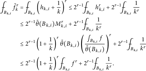 $$ \begin{align*} \frac{\ \ }{\ \ }{\hskip -0.4cm}\int_{B_{k,i}} \tilde{f}_k^r&=\frac{\ \ }{\ \ }{\hskip -0.4cm}\int_{B_{k,i}} \left(h_{k,i}+\frac1k\right)^r\leq 2^{r-1}\frac{\ \ }{\ \ }{\hskip -0.4cm}\int_{B_{k,i}} h_{k,i}^r+2^{r-1}\frac{\ \ }{\ \ }{\hskip -0.4cm}\int_{B_{k,i}} \frac1{k^r}\\ &\leq 2^{r-1}\tilde{\theta}(B_{k,i})M_{k,i}^r+2^{r-1}\frac{\ \ }{\ \ }{\hskip -0.4cm}\int_{B_{k,i}} \frac1{k^r}\\ &\leq 2^{r-1}\left(1+\frac1k\right)^r\tilde{\theta}(B_{k,i}) \left(\frac{\int_{B_{k,i}} f}{\tilde{\theta}(B_{k,i})}\right)^r+2^{r-1}\frac{\ \ }{\ \ }{\hskip -0.4cm}\int_{B_{k,i}} \frac1{k^r}\\ &\leq 2^{r-1}\left(1+\frac1k\right)^r\frac{\ \ }{\ \ }{\hskip -0.4cm}\int_{B_{k,i}} f^r+2^{r-1}\frac{\ \ }{\ \ }{\hskip -0.4cm}\int_{B_{k,i}}\frac1{k^r}. \end{align*} $$
Summing this estimate up for large k and all
 $B_{k,i}$
with
$B_{k,i}$
with
 $B_{k,i}\cap \Psi (z^\bot \cap \mathbb {S}^n,\delta )\neq \emptyset $
, and using that
$B_{k,i}\cap \Psi (z^\bot \cap \mathbb {S}^n,\delta )\neq \emptyset $
, and using that
 $\frac {\ \ }{\ \ }{\hskip -0.4cm}\int _{\mathbb {S}^n}\tilde {f}_k\geq 2^{-1/2}$
for large k, we deduce that
$\frac {\ \ }{\ \ }{\hskip -0.4cm}\int _{\mathbb {S}^n}\tilde {f}_k\geq 2^{-1/2}$
for large k, we deduce that
 $$ \begin{align*}\frac{\ \ }{\ \ }{\hskip -0.4cm}\int_{\Psi(z^\bot\cap \mathbb{S}^n,\delta)} f_k^r\leq \sqrt{2} \frac{\ \ }{\ \ }{\hskip -0.4cm}\int_{\Psi(z^\bot\cap \mathbb{S}^n,\delta)} \tilde{f}_k^r\leq \sqrt{2}\cdot2^{r-1}\left(1+\frac1k\right)^r\frac{\ \ }{\ \ }{\hskip -0.4cm}\int_{\Psi(z^\bot\cap \mathbb{S}^n,2\delta)} f^r+ \sqrt{2}\cdot\frac{2^{r-1}}{k^r}\leq 2^r\varepsilon. \end{align*} $$
For
 $\alpha>0$
and
$\alpha>0$
and
 $p=1-\frac 1\alpha $
, the
$p=1-\frac 1\alpha $
, the
 $L^p$
-surface area
$L^p$
-surface area
 $dS_{\Omega ,p}=u^{1-p}dS_\Omega $
was introduced in the seminal works [Reference Lutwak39–Reference Lutwak41] for a convex body
$dS_{\Omega ,p}=u^{1-p}dS_\Omega $
was introduced in the seminal works [Reference Lutwak39–Reference Lutwak41] for a convex body
 $\Omega \subset \Bbb R^{n+1}$
with
$\Omega \subset \Bbb R^{n+1}$
with
 $o\in \Omega $
and support function u. Since the surface area measure is weakly continuous for
$o\in \Omega $
and support function u. Since the surface area measure is weakly continuous for
 $p<1$
, and if
$p<1$
, and if
 $K\subset \Bbb R^{n+1}$
is an at most n-dimensional compact convex set, then
$K\subset \Bbb R^{n+1}$
is an at most n-dimensional compact convex set, then
 $S_{K,p}\equiv 0$
for
$S_{K,p}\equiv 0$
for
 $p<1$
, we have the following statement.
$p<1$
, we have the following statement.
Lemma 5.2 If convex bodies
 $\Omega _m\subset \Bbb R^{n+1}$
tend to a compact convex set
$\Omega _m\subset \Bbb R^{n+1}$
tend to a compact convex set
 $K\subset \Bbb R^{n+1}$
where
$K\subset \Bbb R^{n+1}$
where
 $o\in \Omega _m,K$
, and
$o\in \Omega _m,K$
, and
 $\liminf _{m\to \infty }S_{\Omega _m,p}>0$
, then
$\liminf _{m\to \infty }S_{\Omega _m,p}>0$
, then
 $\mathrm {int}K\neq \emptyset $
and
$\mathrm {int}K\neq \emptyset $
and
 $S_{\Omega _m,p}$
tends weakly to
$S_{\Omega _m,p}$
tends weakly to
 $S_{K,p}$
.
$S_{K,p}$
.
For the reader’s sake, let us recall Theorem 1.1.
Theorem 5.3 For
 $\alpha>\frac 1{n+2}$
and finite nontrivial Borel measure
$\alpha>\frac 1{n+2}$
and finite nontrivial Borel measure
 $\mu $
on
$\mu $
on
 $\mathbb {S}^n$
,
$\mathbb {S}^n$
,
 $n\geq 1$
, there exists a weak solution of (1.2) provided the following holds:
$n\geq 1$
, there exists a weak solution of (1.2) provided the following holds:
-
(i) If
$\alpha>1$
and
$\mu $
is not concentrated onto any great subsphere
$x^\bot \cap \mathbb {S}^n$
,
$x\in \mathbb {S}^n$
. -
(ii) If
$\alpha =1$
and
$\mu $
satisfies that for any linear
$\ell $
-subspace
$L\subset \Bbb R^{n+1}$
with
$1\leq \ell \leq n$
, we have:-
(a)
$\displaystyle \mu (L\cap \mathbb {S}^n)\leq \frac {\ell }{n+1}\cdot \mu (\mathbb {S}^n)$
; -
(b) equality in (a) for a linear
$\ell $
-subspace
$L\subset \Bbb R^{n+1}$
with
$1\leq d\leq n$
implies the existence of a complementary linear
$(n+1-\ell )$
-subspace
$\widetilde {L}\subset \Bbb R^{n+1}$
such that
$\mathrm {supp}\,\mu \subset L\cup \widetilde {L}$
.
-
-
(iii) If
$\frac 1{n+2}<\alpha <1$
, assume
$d\mu =fd\theta $
for nonnegative
$f\in L^{\frac {n+1}{n+2-\frac 1\alpha }}( \mathbb {S}^n)$
with
$\int _{\mathbb {S}^n}f>0$
.


Proof Let
 $\alpha>\frac 1{n+2}$
. After rescaling, we may assume that the
$\alpha>\frac 1{n+2}$
. After rescaling, we may assume that the
 $\mu $
in (1.2) is a probability measure. We consider the sequence
$\mu $
in (1.2) is a probability measure. We consider the sequence
 $d\mu _k=\frac 1{\omega _n}f_k\,d\theta $
of Lemma 5.1 of Borel probability measures whose weak limit is
$d\mu _k=\frac 1{\omega _n}f_k\,d\theta $
of Lemma 5.1 of Borel probability measures whose weak limit is
 $\mu $
and
$\mu $
and
 $f_k\in C^\infty ( \mathbb {S}^n)$
satisfies
$f_k\in C^\infty ( \mathbb {S}^n)$
satisfies
 $f_k>0$
. For each
$f_k>0$
. For each
 $f_k$
, let
$f_k$
, let
 $\Omega _k\subset \Bbb R^{n+1}$
be the convex body with
$\Omega _k\subset \Bbb R^{n+1}$
be the convex body with
 $o\in \Omega _k$
provided by Theorem 4.1 whose support function
$o\in \Omega _k$
provided by Theorem 4.1 whose support function
 $u_k$
is the solution of the Monge–Ampère equation
$u_k$
is the solution of the Monge–Ampère equation
 $$ \begin{align} u_k^{\frac1\alpha}\,dS_{\Omega_k}=f _k\,d\theta; \end{align} $$
 $\exists \lambda _k>0$
under control, with
$\exists \lambda _k>0$
under control, with
 $|\lambda _k\Omega |=|B(1)|$
,
$|\lambda _k\Omega |=|B(1)|$
,
 $\Omega _k$
satisfies that
$\Omega _k$
satisfies that
 $$ \begin{align} \mathcal{E}_{\alpha, f_k} (\lambda_k\Omega_k)\leq \mathcal{E}_{\alpha, f_k} (B(1)). \end{align} $$
We also need the observations that
 $$ \begin{align} |\Omega_k|=\frac1{n+1}\int_{\mathbb{S}^n}u_k\,dS_{\Omega_k}, \end{align} $$
and if
 $p=1-\frac 1\alpha $
, then
$p=1-\frac 1\alpha $
, then
 $$ \begin{align} S_{\Omega_k,p}(\mathbb{S}^n)=\int_{\mathbb{S}^n}u_k^{1-\frac1\alpha}\,dS_{\Omega_k} =\omega_n\frac{\ \ }{\ \ }{\hskip -0.4cm}\int_{\mathbb{S}^n}f_k=\omega_n. \end{align} $$
We claim that if there exists
 $\Delta>0$
depending on n,
$\Delta>0$
depending on n,
 $\alpha $
, and
$\alpha $
, and
 $\mu $
such that
$\mu $
such that
 $$ \begin{align} \mathrm{diam}\Omega_k\leq \Delta,\ \mbox{then Theorem 5.3 holds.} \end{align} $$
To prove this claim, we note that (5.9) yields the existence of a subsequence of
 $\{\Omega _k\}$
tending to a compact convex set
$\{\Omega _k\}$
tending to a compact convex set
 $\Omega $
with
$\Omega $
with
 $o\in \Omega $
, which is a convex body by (5.8) and Lemma 5.2. Moreover, Lemma 5.2 also yields that
$o\in \Omega $
, which is a convex body by (5.8) and Lemma 5.2. Moreover, Lemma 5.2 also yields that
 $\Omega $
is an Alexandrov solution of (1.2), verifying the claim (5.9).
$\Omega $
is an Alexandrov solution of (1.2), verifying the claim (5.9).
We divide the rest of the argument verifying Theorem 5.3 into three cases.
Case 1:
 $\alpha>1$
.
$\alpha>1$
.
Since
 $\mu $
is not concentrated to any great subsphere, there exist
$\mu $
is not concentrated to any great subsphere, there exist
 $\delta \in (0,\frac 12)$
depending on
$\delta \in (0,\frac 12)$
depending on
 $\mu $
such that
$\mu $
such that
 $\mu \left (\Psi (z^\bot \cap \mathbb {S}^n,2\delta )\right )\leq 1-2\delta $
for any
$\mu \left (\Psi (z^\bot \cap \mathbb {S}^n,2\delta )\right )\leq 1-2\delta $
for any
 $z\in S^{n-1}$
. It follows from Lemma 5.1 that we may assume that
$z\in S^{n-1}$
. It follows from Lemma 5.1 that we may assume that
 $$ \begin{align} \frac{\ \ }{\ \ }{\hskip -0.4cm}\int_{\Psi(z^\bot\cap \mathbb{S}^n,\delta)}f_k\leq 1-\delta \mbox{ for any}\ z\in S^{n-1}. \end{align} $$
Now, Theorem 4.1 implies that
 $\lambda _k\geq c$
for a constant
$\lambda _k\geq c$
for a constant
 $c>0$
depending on n,
$c>0$
depending on n,
 $\delta $
, and
$\delta $
, and
 $\alpha $
, and in turn Theorem 4.1, (4.3), and
$\alpha $
, and in turn Theorem 4.1, (4.3), and
 $\frac 1{\alpha }-1<0$
yield that
$\frac 1{\alpha }-1<0$
yield that
 $$ \begin{align*}\mathcal{E}_{\alpha, f} (\Omega_k)=\frac{\alpha}{\alpha-1}\cdot\log\lambda_k^{\frac1{\alpha}-1} +\mathcal{E}_{\alpha, f} (\lambda_k\Omega_k)\leq \frac{\alpha}{\alpha-1}\cdot\log\lambda_k^{\frac1{\alpha}-1} +\mathcal{E}_{\alpha, f} (B(1))\leq C \end{align*} $$
for a constant
 $C>0$
depending on n,
$C>0$
depending on n,
 $\delta $
, and
$\delta $
, and
 $\alpha $
. Therefore, Theorem 2.1 and (5.10) imply that the sequence
$\alpha $
. Therefore, Theorem 2.1 and (5.10) imply that the sequence
 $\{\Omega _k\}$
is bounded, and in turn the claim (5.9) implies Theorem 5.3 if
$\{\Omega _k\}$
is bounded, and in turn the claim (5.9) implies Theorem 5.3 if
 $\alpha>1$
.
$\alpha>1$
.
Case 2:
 $\alpha =1$
.
$\alpha =1$
.
The argument is by induction on
 $n\geq 0$
where we do not put any restriction on the probability measure
$n\geq 0$
where we do not put any restriction on the probability measure
 $\mu $
in the case
$\mu $
in the case
 $n=0$
. For the case
$n=0$
. For the case
 $n=0$
, we observe that any finite measure
$n=0$
, we observe that any finite measure
 $\mu $
on
$\mu $
on
 $S^0$
can be represented in the form
$S^0$
can be represented in the form
 $d\mu =u\,dS_\Omega $
for a suitable segment
$d\mu =u\,dS_\Omega $
for a suitable segment
 $\Omega \subset \Bbb R^1$
.
$\Omega \subset \Bbb R^1$
.
For the case
 $n\geq 1$
, assuming that we have verified Theorem 5.3(ii) in smaller dimensions, we consider a Borel measure probability
$n\geq 1$
, assuming that we have verified Theorem 5.3(ii) in smaller dimensions, we consider a Borel measure probability
 $\mu $
on
$\mu $
on
 $S^n$
satisfying (a) and (b).
$S^n$
satisfying (a) and (b).
Case 2.1: There exists a linear
 $\ell $
-subspace
$\ell $
-subspace
 $L\subset \Bbb R^{n+1}$
with
$L\subset \Bbb R^{n+1}$
with
 $1\leq \ell \leq n$
and
$1\leq \ell \leq n$
and
 $\mu (L\cap \mathbb {S}^n)= \frac {\ell }{n+1}\cdot \mu (\mathbb {S}^n)$
.
$\mu (L\cap \mathbb {S}^n)= \frac {\ell }{n+1}\cdot \mu (\mathbb {S}^n)$
.
Let
 $\widetilde {L}\subset \Bbb R^{n+1}$
be the complementary linear
$\widetilde {L}\subset \Bbb R^{n+1}$
be the complementary linear
 $(n+1-\ell )$
-subspace with
$(n+1-\ell )$
-subspace with
 $\mathrm {supp}\,\mu \subset L\cup \widetilde {L}$
, and hence
$\mathrm {supp}\,\mu \subset L\cup \widetilde {L}$
, and hence
 $\mu (\widetilde {L}\cap \mathbb {S}^n)= \frac {n+1-\ell }{n+1}\cdot \mu (\mathbb {S}^n)$
. It follows by induction that there exist an
$\mu (\widetilde {L}\cap \mathbb {S}^n)= \frac {n+1-\ell }{n+1}\cdot \mu (\mathbb {S}^n)$
. It follows by induction that there exist an
 $\ell $
-dimensional compact convex set
$\ell $
-dimensional compact convex set
 $K'\subset L$
and an
$K'\subset L$
and an
 $(n+1-\ell )$
-dimensional compact convex set
$(n+1-\ell )$
-dimensional compact convex set
 $\widetilde {K}'\subset \widetilde {L}$
such that
$\widetilde {K}'\subset \widetilde {L}$
such that ![]() and
and ![]() . Finally, for
. Finally, for
 $K=\widetilde {L}^\bot \cap (K'+L^\bot )$
and
$K=\widetilde {L}^\bot \cap (K'+L^\bot )$
and
 $\widetilde {K}=L^\bot \cap (\widetilde {K}'+\widetilde {L}^\bot )$
, there exist
$\widetilde {K}=L^\bot \cap (\widetilde {K}'+\widetilde {L}^\bot )$
, there exist
 $\alpha ,\tilde {\alpha }>0$
such that
$\alpha ,\tilde {\alpha }>0$
such that
 $$ \begin{align*}\mu=(n+1)V_{\alpha K+\tilde{\alpha}\widetilde{K}}. \end{align*} $$
Case 2.2:
 $\mu (L\cap \mathbb {S}^n)< \frac {\ell }{n+1}\cdot \mu (\mathbb {S}^n)$
for any linear
$\mu (L\cap \mathbb {S}^n)< \frac {\ell }{n+1}\cdot \mu (\mathbb {S}^n)$
for any linear
 $\ell $
-subspace
$\ell $
-subspace
 $L\subset \Bbb R^{n+1}$
with
$L\subset \Bbb R^{n+1}$
with
 $1\leq \ell \leq n$
.
$1\leq \ell \leq n$
.
It follows by a compactness argument that there exists
 $\delta \in (0,\frac 12)$
depending on
$\delta \in (0,\frac 12)$
depending on
 $\mu $
such that
$\mu $
such that
 $\mu (\Psi (L\cap \mathbb {S}^n,2\delta ))<(1-2\delta )\cdot \frac {\ell }{n+1}$
for any linear
$\mu (\Psi (L\cap \mathbb {S}^n,2\delta ))<(1-2\delta )\cdot \frac {\ell }{n+1}$
for any linear
 $\ell $
-subspace L of
$\ell $
-subspace L of
 $\Bbb R^{n+1}$
,
$\Bbb R^{n+1}$
,
 $\ell =1,\ldots ,n$
. We consider the sequence of probability measures
$\ell =1,\ldots ,n$
. We consider the sequence of probability measures
 $d\mu _k=\frac 1{\omega _n}f_k\,d\theta $
of Lemma 5.1 tending weakly to
$d\mu _k=\frac 1{\omega _n}f_k\,d\theta $
of Lemma 5.1 tending weakly to
 $\mu $
such that
$\mu $
such that
 $f_k>0$
,
$f_k>0$
,
 $f_k\in C^\infty (\mathbb {S}^n)$
, and
$f_k\in C^\infty (\mathbb {S}^n)$
, and
 $$ \begin{align} \mu_k\left(\Psi\left(L\cap \mathbb{S}^n,\delta\right)\right)<(1-\delta)\cdot \frac{\ell}{n+1} \end{align} $$
for any linear
 $\ell $
-subspace L of
$\ell $
-subspace L of
 $\Bbb R^{n+1}$
,
$\Bbb R^{n+1}$
,
 $\ell =1,\ldots ,n$
.
$\ell =1,\ldots ,n$
.
For each
 $f_k$
, let
$f_k$
, let
 $\Omega _k\subset \Bbb R^{n+1}$
with
$\Omega _k\subset \Bbb R^{n+1}$
with
 $o\in \Omega _k$
be the convex body provided by Theorem 4.1 whose support function
$o\in \Omega _k$
be the convex body provided by Theorem 4.1 whose support function
 $u_k$
is the solution of the Monge–Ampère equation (4.1) and satisfies (4.2) with
$u_k$
is the solution of the Monge–Ampère equation (4.1) and satisfies (4.2) with
 $f=f_k$
and
$f=f_k$
and
 $\lambda =\lambda _k$
where
$\lambda =\lambda _k$
where
 $|B(1)|=|\lambda _k\Omega _k|$
for
$|B(1)|=|\lambda _k\Omega _k|$
for
 $\lambda _k>0$
, and
$\lambda _k>0$
, and
 $$ \begin{align*} |\Omega_k|&=\frac1{n+1}\,\int_{\mathbb{S}^n}u_k\det(\bar{\nabla}^2_{ij} u_k+u_k\bar{g}_{ij})\,d\theta= \frac{\omega_n}{n+1}\,\frac{\ \ }{\ \ }{\hskip -0.4cm}\int_{\mathbb{S}^n}u_k\det(\bar{\nabla}^2_{ij} u_k+u_k\bar{g}_{ij})\\ &=|B(1)|\,\frac{\ \ }{\ \ }{\hskip -0.4cm}\int_{\mathbb{S}^n}f_k=|B(1)|, \end{align*} $$
and hence
 $\lambda _k=1$
. In particular, (4.3) yields
$\lambda _k=1$
. In particular, (4.3) yields
 $$ \begin{align*}\mathcal{E}_{1, f_k} (\lambda_k\Omega_k)\leq \mathcal{E}_{1, f_k} (B(1))\leq \log 2. \end{align*} $$
Since
 $\mathcal {E}_{1, f_k} (\Omega _k)$
is bounded, (5.11) and Theorem 2.1 imply that the sequence
$\mathcal {E}_{1, f_k} (\Omega _k)$
is bounded, (5.11) and Theorem 2.1 imply that the sequence
 $\Omega _k$
stays bounded, as well. Therefore, the claim (5.9) yields Theorem 5.3 if
$\Omega _k$
stays bounded, as well. Therefore, the claim (5.9) yields Theorem 5.3 if
 $\alpha =1$
.
$\alpha =1$
.
Case 3:
 $\frac 1{n+2}<\alpha <1$
.
$\frac 1{n+2}<\alpha <1$
.
We set
 $p=1-\frac 1\alpha \in (-n-1,0)$
and
$p=1-\frac 1\alpha \in (-n-1,0)$
and
 $r=\frac {n+1}{n+1+p}>1$
, and
$r=\frac {n+1}{n+1+p}>1$
, and
 $$ \begin{align} \tau= \frac12\cdot 2^{-\frac{|p|(n+1)}{|p|+n}}, \end{align} $$
and choose
 $\delta \in (0,\frac 12)$
such that
$\delta \in (0,\frac 12)$
such that
 $$ \begin{align*}\frac{\ \ }{\ \ }{\hskip -0.4cm}\int_{\Psi(z^\bot\cap \mathbb{S}^n,2\delta)}f^r\leq \frac{\tau^r}{2^r} \end{align*} $$
for any
 $z\in S^{n-1}$
. We deduce from Lemma 5.1 that if
$z\in S^{n-1}$
. We deduce from Lemma 5.1 that if
 $z\in S^{n-1}$
, then
$z\in S^{n-1}$
, then
 $$ \begin{align} \frac{\ \ }{\ \ }{\hskip -0.4cm}\int_{\Psi(z^\bot\cap \mathbb{S}^n,\delta)}f_k^r\leq \tau^r. \end{align} $$
We deduce from (5.5), (5.7), and
 $|\lambda _k\Omega _k|=|B(1)|=\frac {\omega _n}{n+1}$
that
$|\lambda _k\Omega _k|=|B(1)|=\frac {\omega _n}{n+1}$
that
 $$ \begin{align} \frac{\ \ }{\ \ }{\hskip -0.4cm}\int_{\mathbb{S}^n}u_k^{p}f_k=\frac{n+1}{\omega_n} \int_{\mathbb{S}^n}u_k\,dS_{\Omega_k}= \frac{n+1}{\omega_n}\,|\Omega_k|=\lambda_k^{-n-1}. \end{align} $$
In particular, (4.3) and the upper bound on the entropy yield that
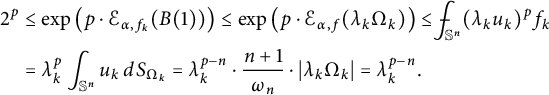 $$ \begin{align} \nonumber 2^{p}&\leq \exp\left(p\cdot \mathcal{E}_{\alpha, f_k} (B(1))\right) \leq \exp\left(p\cdot \mathcal{E}_{\alpha, f} (\lambda_k\Omega_k)\right) \leq \frac{\ \ }{\ \ }{\hskip -0.4cm}\int_{\mathbb{S}^n}(\lambda_ku_k)^{p}f_k\\ &=\lambda_k^{p}\int_{\mathbb{S}^n}u_k\,dS_{\Omega_k}= \lambda_k^{p-n}\cdot\frac{n+1}{\omega_n}\cdot|\lambda_k\Omega_k|=\lambda_k^{p-n}. \end{align} $$
It follows from (5.15) that
 $\lambda _k\leq 2^{\frac {|p|}{|p|+n}}$
, and in turn (5.14) yields that
$\lambda _k\leq 2^{\frac {|p|}{|p|+n}}$
, and in turn (5.14) yields that
 $$ \begin{align*}\frac{\ \ }{\ \ }{\hskip -0.4cm}\int_{\mathbb{S}^n}u_k^{p}f_k\geq 2^{-\frac{|p|(n+1)}{|p|+n}}. \end{align*} $$
Therefore,
 $\tau \leq \frac 12\frac {\ \ }{\ \ }{\hskip -0.4cm}\int _{\mathbb {S}^n}u_k^{p}f_k$
(cf. (5.12)), (5.13), and Theorem 2.1 yield that the sequence
$\tau \leq \frac 12\frac {\ \ }{\ \ }{\hskip -0.4cm}\int _{\mathbb {S}^n}u_k^{p}f_k$
(cf. (5.12)), (5.13), and Theorem 2.1 yield that the sequence
 $\{\Omega _k\}$
is bounded, and in turn the claim (5.9) implies Theorem 5.3 if
$\{\Omega _k\}$
is bounded, and in turn the claim (5.9) implies Theorem 5.3 if
 $\frac 1{n+2}<\alpha <1$
.
$\frac 1{n+2}<\alpha <1$
.


 Open access