Relative fluid stretching and rotation for sparse trajectory observations

Abstract

As most mathematically justifiable Lagrangian coherent structure detection methods rely on spatial derivatives, their applicability to sparse trajectory data has been limited. For experimental fluid dynamicists and natural scientists working with Lagrangian trajectory data via passive tracers in unsteady flows (e.g. Lagrangian particle tracking or ocean buoys), obtaining material measures of fluid rotation or stretching is an active topic of research. To facilitate frame-indifferent investigations in unsteady and sparsely sampled flows, we present a novel approach to quantify fluid stretching and rotation via relative Lagrangian velocities. This technique provides a formal objective extension of quasi-objective metrics to unsteady flows by accounting for mean flow behaviour. For extremely sparse experimental data, fluid structures may be significantly undersampled and the mean flow behaviour becomes difficult to quantify. We provide a means to maintain the accuracy of our novel sparse flow diagnostics in extremely sparse sampling scenarios, such as ocean buoy data and Lagrangian particle tracking. We use data from multiple numerical and experimental flows to show that our methods can identify structures beyond existing limits of sparse, frame-indifferent diagnostics and exhibit improved interpretability over common frame-dependent diagnostics.

1. Introduction

Experimental methods for spatially and temporally resolving fluid velocities in both large and natural flow domains have improved significantly in recent years. For a wide range of turbulent flows, ground truth measurements of fluid velocity can be measured using high-speed imaging of advected particles and any number of particle image velocimetry (PIV) and Lagrangian particle tracking (LPT) algorithms. For the largest spatial scales and for the sparsest trajectory data, only LPT is suitable and provides a Lagrangian framework with which to extract transport features in the flow. At oceanographic and atmospheric circulation spatial scales, GPS tracking of buoys and balloons typically replaces PIV and LPT imaging approaches. To date, Lagrangian data have provided great insights to our studies of sea ice and ocean dynamics, as well as for meteorologists studying atmospheric behaviours with drifting weather-balloon measurements (Businger, Johnson & Talbot 2006; Leppäranta 2011; van Sebille et al. 2018). Coherent structure identification from sparse data, however, has typically relied on a grab-bag of techniques, often tailored to each individual flow, with no unifying metrics that work in all domains.

Historically, lab-based measurement techniques have evolved hand-in-hand with systematic technological advances such as integrated circuits, the laser and most recently the CMOS chip. Starting out from intrusive, probe-based extraction of Eulerian data (fixed-point statistics) through to time-averaged planar field measurements, e.g. PIV, and then most recently to dense time-resolved particle tracking in three dimensions, the availability of said tools has influenced the choice of metrics used to describe the flow in question. As a case in point, the use of Reynolds stresses to describe shear flows has dominated the community since the days of hot-wire anemometry even though such stresses are only a proxy to the coherent structures driving the turbulent processes on hand.

Commonly used approaches for identifying structures in experimental flows are typically frame-dependent. That is, the extracted features will depend on the choice of reference frame of the experimentalist and, thus, violate a fundamental requirement from continuum mechanics for describing material fluid behaviour. Material behaviour can be thought of as the features in a flow revealed in a tracer visualisation experiment (e.g. dye or smoke). Although our physical intuition around Lagrangian velocities may be strong, e.g. one can easily imagine a leaf floating downstream on a river surface, extracting physically meaningful diagnostics that describe the material deformation of the surrounding fluid is much more difficult. Indeed, many common and intuitive trajectory metrics are frame-dependent, such as the Lagrangian velocity, looping (Lumpkin 2016), curvature (Bristow et al. 2023), complexity measures (Rypina et al. 2011) and network-based approaches (Iacobello & Rival 2023), as well as many diagnostics from gridded velocity data such as vorticity (Bernard & Thomas 1993), swirling strength (Zhou et al. 1999) and the lambda-2 criterion (Jeong & Hussain 1995) .

Although choosing a single common reference frame may appear logical to study flows we understand well, this approach quickly loses its foundation when encountering flows where no a priori knowledge of the relevant structures or a natural reference frame are available. Furthermore, truly material behaviour does not change under rigid-body frame changes, regardless of whether a user-preferred frame exists or not (Truesdell & Noll 2004). Thus, Euclidean frame-indifference is a fundamental litmus test for structure identification schemes to actually identify material features even if one always conducts their research in the same reference frame.

Methods that can effectively reveal fluid structures at both high and low trajectory densities, in a frame-independent manner, and for the widest variety of flows would provide a wealth of information for both understanding fluids in observational environments and as a common ground for comparison with numerical simulations. In order to test sparse diagnostics in very different flows, we quantify the sparsity of a data set by normalising the number of trajectories by the square or cube of a characteristic length scale of the flow $\ell$, for two-dimensional (2-D) and three-dimensional (3-D) examples, respectively.

Frame-indifferent (objective) diagnostics that identify Lagrangian coherent structures (LCS) have been developed extensively over the last two decades (see Haller 2023) but their implementation relies on spatial derivatives that are difficult to accurately compute from sparse or unstructured data. To account for this, adaptations have been developed to allow for data sparsity (Lekien & Ross 2010; Rypina et al. 2021; Mowlavi et al. 2022) as have Green’s theorem-based approximations of rate-of-strain metrics from trajectory arrays (Kwok et al. 1990). Most notably, Mowlavi et al. (2022) compared multiple sparse methods for identifying hyperbolic (stretching) and elliptic (rotating) LCS in the Bickley jet and ABC flow. When initialising particles on a structured grid, Mowlavi et al. (2022) were able to accurately cluster particles into elliptic LCS at particle concentrations of $85\ell ^{-2}$ and $504\ell ^{-3}$ for the Bickley jet and ABC flow ($\ell ={\rm \pi}$ for both), respectively. They were also able to identify hyperbolic structures from randomly initialised particles at concentrations of $471\ell ^{-2}$, and $3870\ell ^{-3}$ for the Bickley jet and ABC flow, respectively.

Modern clustering methods provide a complementary frame-indifferent approach to identify regions of fluid with similar fluid particle trajectories (see, e.g. Froyland & Padberg-Gehle 2015; Hadjighasem et al. 2016; Schlueter-Kuck & Dabiri 2017). Graph-theory-based clustering algorithms quantify similarity between trajectories themselves and, thus, do not require measurements to be spatially proximal, as is required for gradient-reliant approaches. As such, trajectories can be generated from gridded flow data or observed experimentally, such as by LPT. In contrast to hyperbolic and elliptic LCS, the coherent structures identified with trajectory clustering algorithms have no inherent physical meaning besides a certain trajectory similarity. That is, one cannot use clustering alone to interpret local stretching or rotation rates without a priori knowledge of the flow behaviour.

The squared relative dispersion ($d^2$) is an outlier diagnostic as it is suitable for sparse and randomly oriented trajectories, is also objective (Haller & Yuan 2000), and has been developed with a strong physical foundation. This fluid stretching metric has been used for a number of years, particularly to understand dispersion and mixing by oceanographers in a statistical manner (LaCasce 2008). The ability of $d^2$ to identify coherent structures, however, is limited as one is forced to initially choose particle pairs, whose relative motion inevitably becomes uncorrelated at an a priori unknown temporal horizon (Haller, Aksamit & Bartos 2021).

Current approaches for physically meaningful sparse trajectory diagnostics still rely on a relatively dense field of particles (for a comparison, see, e.g. Mowlavi et al. 2022), or well-behaved trajectory array geometries (Lindsay & Stern 2003). In light of the unstructured nature of trajectory data, it is more common for experimental LPT data to be spatially and temporally averaged or assimilated into gridded products prior to structure analysis (Schröder & Schanz 2023). When averaging or projecting time-dependent fluid motions to a single instance in time, such approaches potentially oversimplify transient (non-stationary) flow behaviour that may exist in the underlying Lagrangian data.

Complementing these sparse approaches is the recent development of quasi-objective coherent structure diagnostics, the trajectory rotation average (TRA) and trajectory stretching exponent (TSE) (Haller et al. 2021). TSE and TRA calculate stretching and rotation, respectively, for individual particle trajectories with no requirement of nearby velocity or trajectory data. The authors mathematically proved that under suitable conditions (slowly varying, relatively small mean vorticity) TRA and TSE approximate objective measures of rotation and stretching. Given these flow conditions, TRA and TSE have proven to be advantageous in several extremely sparse geophysical buoy experiments, accurately identifying algae trapping eddies in the ocean (Encinas-Bartos, Aksamit & Haller 2022), as well as predicting Arctic sea ice stretching and breakup events that were missed by other approaches (Aksamit et al. 2023).

In the present research, we introduce relative stretching and rotation metrics for individual trajectories that incorporate knowledge of the average translation and rotation of the sampled fluid. By utilising bulk behaviour of concurrent trajectories in a given experiment, we can obtain objective diagnostics of stretching and rotation in unsteady flows with much of the same flexibility of a true single-trajectory method. Our measures of relative stretching and rotation can be seen as a natural synthesis of the objective Eulerian deformation velocity of Kaszás, Pedergnana & Haller (2023) and quasi-objective diagnostics of Haller et al. (2021).

In the following, we develop the theory of relative stretching and rotation and provide several examples of performance. The robustness of relative Lagrangian stretching and rotation is displayed by first comparing full resolution structure topology against ground truth LCS boundaries in 2-D and 3-D flows, and then testing the accuracy of the trajectory diagnostics in progressively downsampled data sets. We also display the enhanced ability of relative rotation to distinguish between experimental turbulent flows for extremely sparsely sampled data, when compared with traditional metrics. This superior performance is shown for numerical simulation data and in real-world observations of ocean buoys from the global drifter database and a large-scale LPT wind tunnel experiment.

2. Methods

2.1. Background

Consider a fluid flow with time-varying velocity field $\boldsymbol {v}(\boldsymbol {x},t)$. Infinitesimal fluid particle trajectories can be generated as solutions to the differential equation $\dot {\boldsymbol {x}}(t)=\boldsymbol {v}(\boldsymbol {x}(t),t)$ from some initial position $\boldsymbol {x}(t_0)=\boldsymbol {x}_0$. The flow map $\boldsymbol {F}$ maps fluid particles from their time $t_0$-positions to their position at a time $t$, along the trajectory $\boldsymbol {x}(t; t_0, \boldsymbol {x}_0)$,

(2.1)\begin{equation} \boldsymbol{F}_{t_0}^t: \boldsymbol{x}_0\mapsto \boldsymbol{x}(t; t_0, \boldsymbol{x}_0). \end{equation}

The measurement of a scalar quantity associated to a fluid particle $P(\boldsymbol {x}(t))$, such as its temperature, is objective (frame-indifferent) under Euclidean transformations of the form

(2.2)\begin{equation} \boldsymbol{x}=\boldsymbol{Q}(t)\boldsymbol{y}+\boldsymbol{b}(t), \end{equation}

where $\boldsymbol {Q}(t)$ is a rigid-body rotation matrix (an element of the matrix group $\mathrm {SO}(n)$ for $n=2$ or $3$) and $\boldsymbol {b}(t)$ is a time-varying translation vector. That is, in the two reference frames, the scalar quantity remains the same: $\tilde {P}(\boldsymbol {y})=P(\boldsymbol {x})$, where $P$ and $\tilde {P}$ are measured in the original and translated frames, respectively.

Similarly, one can define an objective Lagrangian vector $\boldsymbol {\xi }$ as one that transforms under (2.2) as

(2.3)\begin{equation} \tilde{\boldsymbol{\xi}}(\boldsymbol{y}(t,\boldsymbol{y}_0)) = \boldsymbol{Q}^T(t)\boldsymbol{\xi}(\boldsymbol{x}(t,\boldsymbol{x}_0)). \end{equation}

To reveal the ground-truth material fluid structures undergoing significant stretching and rotation, we will rely on the frame-indifferent finite-time Lyapunov exponent (FTLE) (Haller 2015) and the Lagrangian-averaged vorticity deviation (LAVD) (Haller et al. 2016), respectively:

(2.4)\begin{gather} \mathrm{FTLE}_{t_{0}}^{t}(\boldsymbol{x}_{0})=\frac{1}{2\left|t-t_{0}\right|}\log\lambda_{{max}}(\boldsymbol{C}_{t_0}^t(\boldsymbol{x}_{0})), \end{gather}

(2.5)\begin{gather}\mathrm{LAVD}_{t_{0}}^{t}(\boldsymbol{x}_{0})=\frac{1}{|t-t_{0}|}\int_{t_{0}}^{t}\left|\boldsymbol{\omega}(\boldsymbol{F}_{t_0}^s(\boldsymbol{x}_{0}),s)-\bar{\boldsymbol{\omega}}(s)\right|\,{\rm d}s, \end{gather}

where $\lambda _{{max}}>0$ is the largest eigenvalue of the positive-definite tensor $\boldsymbol {C}_{t_0}^t=[\boldsymbol {\nabla }\boldsymbol {F}_{t_0}^t]^{\mathrm {T}}\boldsymbol {\nabla }\boldsymbol {F}_{t_0}^t$ and $\bar {\boldsymbol {\omega }}$ is the time-varying but spatially averaged vorticity. Although LAVD and FLTE have seen widespread use in studies of atmospheric, oceanic and experimental flows, their direct application to sparse data sets has been hindered by their strong reliance on velocity and flow map gradients.

In the sparse sampling context, where we have no control over trajectory densities or orientations, it would be advantageous to develop a LCS algorithm based on individual trajectories. The primary issue surrounding the development of an objective single-trajectory diagnostic is that one can always pass to the frame of the particle, and in that reference frame, the particle is not moving. As a way around this frame-dependency, Haller et al. (2021) recently developed the quasi-objective coherent structure diagnostics

(2.6)\begin{gather} \overline{\mathrm{TSE}}_{t_0}^{t_N}(\boldsymbol{x}_0)=\frac{1}{t_N-t_0}\sum_{j=0}^{N-1}\left |\log\frac{|{\dot{\boldsymbol{x}}}(t_{j+1})|}{|{\dot{\boldsymbol{x}}}(t_{j})|} \right|, \end{gather}

(2.7)\begin{gather}\overline{\mathrm{TRA}}_{t_0}^{t_N}(\boldsymbol{x}_0) = \frac{1}{t_N-t_0}\sum_{j=0}^{N-1}\cos^{{-}1}\frac{\langle \dot{\boldsymbol{x}}(t_j), \dot{\boldsymbol{x}}(t_{j+1}) \rangle} {|\dot{\boldsymbol{x}}(t_j)| |\dot{\boldsymbol{x}}(t_{j+1})|}, \end{gather}

which provide close approximations to objective stretching and rotation measures if the Lagrangian trajectories are analysed in slowly varying references frames with relatively small mean vorticity.

In the following, we derive the experiment-relative Lagrangian velocity of a fluid particle and show that it is an objective vector. With these relative velocities, we can objectively define the relative stretching and rotation of fluid from sparsely sampled experimental data, with no a priori knowledge of the structures being investigated.

2.2. Relative Lagrangian velocity

Suppose we have a collection of Lagrangian particle trajectory observations $\{\boldsymbol {x}_i(t)\}$, with corresponding velocities along their trajectories $\dot {\boldsymbol {x}}_i(t)=\boldsymbol {v}_i(t)$. By linearity of the time derivative, the velocity of the average position of these particles at time $t$ is equivalent to the average of their Lagrangian velocities,

(2.8)\begin{gather} \bar{\boldsymbol{x}}(t)=\frac{1}{n}\sum_{i=1}^n \boldsymbol{x}_i(t), \end{gather}

(2.9)\begin{gather} \boldsymbol{v}(t)=\dot{\boldsymbol{x}}(t), \quad \bar{\boldsymbol{v}}(t)=\frac{1}{n}\sum_{i=1}^n \boldsymbol{v}_i(t)=\dot{\bar{\boldsymbol{x}}}(t). \end{gather}

Furthermore, define the time-varying moment-of-inertia tensor

(2.10)\begin{equation} {\textsf{$\mathit{\Theta}$}}(t)=\overline{|\boldsymbol{x}_i-\overline{\boldsymbol{x}}|^2\boldsymbol{\mathsf{I}}-(\boldsymbol{x}_i-\overline{\boldsymbol{x}})\otimes(\boldsymbol{x}_i-\overline{\boldsymbol{x}})}, \end{equation}

where averaging is over the trajectory index $i$. From our collection of trajectories, mimicking the Eulerian calculations of Kaszás et al. (2023), we relate the experiment-based vorticity to the approximate rigid-body rotation of the flow as

(2.11)\begin{equation} \overline{\boldsymbol{\omega}}_{rb}(t)={\textsf{$\mathit{\Theta}$}}^{{-}1}\overline{(\boldsymbol{x}_i-\overline{\boldsymbol{x}})\times(\boldsymbol{v}_i-\overline{\boldsymbol{v}})}. \end{equation}

To avoid cumbersome notation, we drop the subscript $i$ from hereon when it is clear we are referring to a specific trajectory $\boldsymbol {x}(t; t_0, \boldsymbol {x}_0)$. Having now calculated the average rotation and translation of the sampled fluid in our experiment, we define the relative velocity along a Lagrangian trajectory as

(2.12)\begin{equation} \boldsymbol{v}_d(\boldsymbol{x}(t))=\boldsymbol{v}(\boldsymbol{x}(t))-\bar{\boldsymbol{v}}(t) - \overline{\boldsymbol{\omega}}_{rb}(t)\times(\boldsymbol{x}-\bar{\boldsymbol{x}}). \end{equation}

The objectivity of $\boldsymbol {v}_d$, and scalar diagnostics generated from it, follows from the objectivity of $\boldsymbol {v}_d$ originally derived by Kaszás et al. (2023). That is, by removing the mean rate of translation and rotation of our trajectory observations, we can study objective properties of dynamic fluid structures in our sampled domain.

This is a Lagrangian-observation-based implementation of the Eulerian deformation velocity $\boldsymbol {v}_d$ originally derived by Kaszás et al. (2023). This is, however, distinct from calculating Lagrangian trajectories in time-resolved Eulerian $\boldsymbol {v}_d$ fields. Trajectories calculated in the Eulerian $\boldsymbol {v}_d$ do not necessarily trace material flow features, but observed experimental tracers will (Kaszás et al. 2023). Instead, $\boldsymbol {v}_d$ can be used to objectivise frame-dependent Eulerian diagnostics in each snapshot. Here, by estimating rigid-body translation and rotation from passive Lagrangian measurements, the relative Lagrangian velocity $\boldsymbol {v}_d$ provides a means to objectivise trajectory diagnostics relative to the sparse data available without a priori knowledge of the underlying flow.

2.3. Stretching

For steady flows, Haller et al. (2021) showed that cumulative fluid stretching and compression normal to trajectories can be quantified using $\overline {\mathrm {TSE}}$ (2.6). In slowly varying flows, this trajectory stretching and compression approximates the true material deformation with the difference being a function of $\partial _t\boldsymbol {v}(\boldsymbol {x}(t),t)$. Furthermore, TSEs were shown to faithfully highlight hyperbolic LCS and reproduce the dominant features of FTLE fields.

Here, we seek a measure of fluid stretching that is frame-indifferent in unsteady flows and has minimal dependence on trajectory concentration, thus making it suitable for extremely sparse sampling in many natural environments. To do this, we introduce the stretching of fluid parcels relative to the bulk behaviour of our flow through the stretching of relative Lagrangian velocity vectors. Formally, the relative trajectory stretching exponents (rTSE and $\mathrm {r}\overline {\mathrm {TSE}}$) from time $t_0$ to time $t_N$ can be written as

(2.13)\begin{gather} \mathrm{rTSE}_{t_0}^{t_N}(\boldsymbol{x}_i) =\frac{1}{t_N-t_0}\log\frac{|\boldsymbol{v}_d({\boldsymbol{x}}_i(t_N))|}{|\boldsymbol{v}_d({\boldsymbol{x}_i}(t_0))|} , \end{gather}

(2.14)\begin{gather}\mathrm{r}\overline{\mathrm{TSE}}_{t_0}^{t_N}(\boldsymbol{x}_i)=\frac{1}{t_N-t_0}\sum_{j=0}^{N-1}\left |\log\frac{|\boldsymbol{v}_d({\boldsymbol{x}}_i(t_{j+1}))|}{|\boldsymbol{v}_d({\boldsymbol{x}}_i(t_{j}))|} \right|. \end{gather}

The $\mathrm {rTSE}$ diagnostic provides the stretching exponent for the relative Lagrangian velocity vector from time $t_0$ to $t_N$, whereas $\mathrm {r}\overline {\mathrm {TSE}}$ is a cumulative measure of all stretching and contraction that occurs in the same time window. Given the objectivity of the relative Lagrangian velocity $\boldsymbol {v}_d$ defined in (2.12), then $\mathrm {rTSE}$ and $\mathrm {r}\overline {\mathrm {TSE}}$ are also objective. That is, because $\hat {\boldsymbol {v}}_d(\boldsymbol {y}(t))=Q^T\boldsymbol {v}_d(\boldsymbol {x}(t))$, we have $|\hat {\boldsymbol {v}}_d(\boldsymbol {y}(t))|=|\boldsymbol {v}_d(\boldsymbol {x}(t))|$ and rTSEs do not change between reference frames. This provides a formal and fully objective extension of the quasi-objective TSEs from Haller et al. (2021) that works in unsteady (time-varying) flows.

2.4. Rotation

For steady flows with negligible mean vorticity, Haller et al. (2021) also derived TRA and ($\overline {\mathrm {TRA}}$), which measures trajectory rotation and successfully identifies elliptic LCS. Under these flow assumptions, $\overline {\mathrm {TRA}}$ calculates the cumulative rotation of material streamline tangent vectors. For highly unsteady, or strongly rotational flows this approach is insufficient as streamlines no longer resemble material lines. Instead, we adopt the average rotation speed of material tangent vectors for relative Lagrangian velocities.

For a given relative Lagrangian velocity vector $\boldsymbol {v}_d$, we can define the unit vector pointing in that direction:

(2.15)\begin{equation} \boldsymbol{e}(t)=\frac{\boldsymbol{v}_d(t)}{| \boldsymbol{v}_d(t)|}. \end{equation}

Then,

(2.16)\begin{equation} {\mathrm{r}\alpha}_{t_0}^{t_N}=\frac{1}{t_N-t_0}\int_{t_0}^{t_N}\left| \dot{\boldsymbol{e}}(t) - \frac{1}{2}\bar{\boldsymbol{\omega}}_{rb}(t)\times\boldsymbol{e}(t)\right|\,{\rm d}t \end{equation}

is an objective measure of the average rotation speed of $\boldsymbol {v}_d$ from time $t_0$ to $t_N$ (Haller et al. 2021). The instantaneous limit of (2.16) also exists ($\alpha _{t_0}=\lim _{t_N\to t_0}\alpha _{t_0}^{t_N}$) and provides the instantaneous rate of rotation of the relative Lagrangian velocity vector with respect to the spatially averaged rotation. Furthermore, for a generic parameterised curve $\gamma$ in three dimensions with a unit tangent velocity vector $\boldsymbol {e}$, the curvature of $\gamma$ is $\dot {\boldsymbol {e}}(t)$. Thus, ${\mathrm {r}\alpha }$ is intrinsically related to classical notions of geometry of flow structures as a form of integrated curvature that accounts for rotation of the surrounding fluid as well.

2.5. Extremely sparse sampling

As we show in the following sections, calculating $\bar {\boldsymbol {v}}(t)$ and $\bar {\boldsymbol {\omega }}(t)$ directly from trajectory data can become problematic at extremely sparse trajectory concentrations. By extremely sparse, we refer to trajectory concentrations less than $1\ell ^{-2}$ and $1\ell ^{-3}$, where $\ell$ is a characteristic length of structures in the flow (e.g. eddy length scale, obstruction dimensions). At this lower limit of trajectory concentration, we are fundamentally undersampling the prominent structures in the flow, and an accurate time-resolved depiction of spatially averaged flow behaviour is not reasonably expected.

That is, $\boldsymbol {\overline {\omega }}_{rb}(t)$ and $\boldsymbol {\bar {v}}(t)$ may start to display strong oscillations in time that are not representative of the underlying mean flow properties. These oscillations contribute unphysical fluctuations in $\boldsymbol {v}_{d}$ and hinder our interpretation of relative stretching and rotation diagnostics. Oscillations can also be easily created by a small number of trajectories leaving the observation domain when only a small total are being measured. An example of this is shown in detail in § 3.1.2.

For these sparse situations, we suggest replacing the time-dependent bulk values $\boldsymbol {\overline {\omega }}_{rb},\boldsymbol {\bar {v}}, \boldsymbol {\bar {x}}$ from ((2.8)–(2.11)) with their temporal averages over the integration window as follows:

(2.17)\begin{gather} \boldsymbol{v}_{{ref}} = \dfrac{1}{t_1-t_0}\int_{t_0}^{t_1} \boldsymbol{\bar{v}}(t)\,{\rm d}t, \end{gather}

(2.18)\begin{gather}\boldsymbol{\omega}_{{ref}} = \dfrac{1}{t_1-t_0}\int_{t_0}^{t_1} \boldsymbol{\overline{\omega}}_{rb}(t)\,{\rm d}t, \end{gather}

(2.19)\begin{gather}\boldsymbol{x}_{{ref}} = \dfrac{1}{t_1-t_0}\int_{t_0}^{t_1}\boldsymbol{\bar{x}}(t)\,{\rm d}t. \end{gather}

While potentially oversimplifying non-stationary oscillations that naturally occur in the flow, using these time-averages provides a smooth estimate of total bulk motion for the time windows in which we are interested. We can then write the Lagrangian velocity relative to this prescribed reference frame as

(2.20)\begin{equation} \boldsymbol{v}_{d{,ref}}(\boldsymbol{x}(t))=\boldsymbol{v}(\boldsymbol{x}(t))-\boldsymbol{v}_{{ref}}(t) - \boldsymbol{\omega}_{{ref}}(t)\times(\boldsymbol{x}-\boldsymbol{x}_{{ref}}), \end{equation}

where $\boldsymbol {v}_{{ref}}$ and $\boldsymbol {\omega }_{{ref}}$ are steady approximations of the bulk translation and rotation in the flow that are informed directly from flow measurements. This extremely sparse data handling is tested for multiple flows in the following sections, as is its ability to recreate accurate full-resolution ${\mathrm {r}\alpha }$ values. Since we are explicitly keeping track of a given choice of reference frame in (2.20), $\boldsymbol {v}_{d{,ref}}$, ${\rm r}\overline {\mathrm {TSE}}$ and ${\mathrm {r}\alpha }$ remain objective and indifferent to Euclidean frame changes.

If additional sources of velocity measurements are available, such as those from anemometers, remotely sensed ocean currents or wind tunnel probes, one may also estimate $\boldsymbol {v}_{{ref}}$ and $\boldsymbol {\omega }_{{ref}}$ from those data, but this approach is not tested herein and should only be considered with caution. Using additional data sources to estimate bulk rigid-body rotation and translation is subject to errors, such as local fluctuations or imperfect placement in the flow, that are not discussed in the present work.

If one imposes $\boldsymbol {v}_{{ref}}=0$, and $\boldsymbol {\omega }_{{ref}}=0$, we can see that TRA and TSE are actually special cases of $\mathrm {r}\alpha$ and $\mathrm {rTSE}$. The present work, therefore, seeks to extend the prior success found by Haller et al. (2021) and Encinas-Bartos et al. (2022) with TRA and TSE to unsteady, time-varying flows. Further, the generalised relative Lagrangian velocity frameworks allows researchers to transparently maintain objectivity if a given reference frame is preferred.

3. Results

We now provide examples of ${\mathrm {r}\alpha }$ and $\mathrm {r}\overline {\mathrm {TSE}}$ analysis for numerical simulations and experimental observations. We evaluate our newly proposed metrics against an array of diagnostics suitable for different experimental flows, with each example detailing a specific advantage of ${\mathrm {r}\alpha }$ and/or $\mathrm {r}\overline {\mathrm {TSE}}$ over prior approaches.

3.1. Numerical simulations

3.1.1. Unsteady Bickley jet

For our first example we consider the unsteady Bickley jet. This is a 2-D geophysical model of a quasi-periodic zonal jet with adjacent migrating eddies whose Lagrangian dynamics have been studied in depth (see, e.g. Del-Castillo-Negrete & Morrison 1993; Rypina et al. 2007). This flow was also used as a benchmark for previous LCS comparisons (Hadjighasem et al. 2017). Its time-dependent stream function is given by

(3.1)\begin{equation} \psi(x,y,t) ={-}UL\tanh\left(\frac{y}{L}\right) + UL\,{\rm sech}^2\left(\frac{y}{L}\right)Re\left[\sum_{n=1}^3 \epsilon_n\exp(-{\rm i}k_nc_nt)\exp({\rm i}k_nx)\right]. \end{equation}

We use the parameters from Rypina et al. (2007) found in table 1.

Table 1. Bickley jet model parameters.

In figure 1 we compare ${\mathrm {r}\alpha }$ and ${\rm r}\overline {\mathrm {TSE}}$ with benchmarks of material rotation and stretching, the LAVD (Haller et al. 2016) and the FTLE (Haller 2015) on a dense grid of trajectories ($3600\ell ^{-2}$, $\ell ={\rm \pi}$), for an integration time of 30 days. This corresponds with approximately six full rotations and significant translation for the advected eddies. We find that ${\mathrm {r}\alpha }$ is able to match the prominent features of the LAVD field by effectively identifying eddies boundaries as closed convex contours and separating them from the central jet. The ${\rm r}\overline {\mathrm {TSE}}$ ridges identify the edges of the central jet and edges of vortices as regions of significant stretching, similar to FTLE. Deviations primarily exist in the centres of the vortex cores where $\boldsymbol {v}_d(\boldsymbol {x}(t))$ does not evolve in a material way.

Figure 1. Evaluation of $\mathrm {r}\alpha$ and $\mathrm {r}\overline {\mathrm {TSE}}$ (a,d) with material rotation (LAVD) and stretching (FTLE) (b,e), and traditional quasi-objective single trajectory diagnostics $\overline {\mathrm {TRA}}$ and $\overline {\mathrm {TSE}}$ (c,f), in the unsteady Bickley jet. Note the distinct central jet with rotating eddies on either side. Here $\overline {\mathrm {TRA}}$ and $\overline {\mathrm {TSE}}$ have difficulty accurately capturing material behaviour (stretching and rotation) due to the large bulk advection in the flow and temporal variability in the velocity field.

Previous work has shown how $\overline {\mathrm {TRA}}$ and $\overline {\mathrm {TSE}}$ can effectively reproduce the same LCS as LAVD and FTLE in slowly varying flows (Haller et al. 2021). In figure 1, we reveal how necessary this slowly varying assumption truly is. With the parameters in table 1, the Bickley jet is highly unsteady. For meaningful quasi-objective calculations, one requires $|\boldsymbol {v}_t|/|\ddot {\boldsymbol {x}}|<<1$, but only $41\,\%$ of trajectories experience $|\boldsymbol {v}_t|/|\ddot {\boldsymbol {x}}|<1$ and only $0.03\,\%$ of particle paths show $|\boldsymbol {v}_t|/|\ddot {\boldsymbol {x}}|<0.1$. This suggests that the coherent structures in this flow are likely evolving or travelling much faster than a Lagrangian particle is able to trace them out. In fact, $\overline {\mathrm {TRA}}$ designates the eddies in figure 1 as exhibiting relatively low rotation. In addition, $\overline {\mathrm {TSE}}$ also suggests nearly everything outside the central jet is undergoing significant stretching, in contrast to the thin hyperbolic regions seen as FTLE ridges. For this degree of unsteadiness and strong eddy advection, ${\mathrm {r}\alpha }$ and ${\rm r}\overline {\mathrm {TSE}}$ are more suitable than $\overline {\mathrm {TRA}}$ and $\overline {\mathrm {TSE}}$ for quantifying fluid rotation and stretching while requiring much less-structured data than LAVD and FTLE.

We now progressively and randomly downsample the number of trajectories to test the robustness of our objective diagnostics at low trajectory densities. In figure 2, we calculate ${\mathrm {r}\alpha }$ and ${\rm r}\overline {\mathrm {TSE}}$ as well as the particle trajectory length (Mancho et al. 2013) and initial particle speed $|\boldsymbol {v}(t_0)|$. Although trajectory length and particle speed are not objective, they are either easily computed or commonly used diagnostics for experimental LPT studies (see, e.g. Fu, Biwole & Mathis 2015; Tauro, Piscopia & Grimaldi 2017; Rosi & Rival 2018). After calculating each diagnostic, we reconstruct the full-resolution diagnostic field using radial basis functions, similar to Encinas-Bartos et al. (2022). In addition, we include the outermost closed convex LAVD contours from figure 1 as a visual reference to aid in the comparisons.

Figure 2. Comparison of relative rotation (${\mathrm {r}\alpha }$) and stretching ($\mathrm {r}\overline {\mathrm {TSE}}$) with non-objective trajectory length and initial particle speed diagnostics. Each diagnostic was progressively and randomly downsampled with the full-resolution product created using radial basis functions. For each panel, we include the outermost closed convex LAVD contours to highlight relative agreement of each sparse diagnostic with ground-truth material rotation.

At a trajectory concentration of 360$\ell ^{-2}$, ${\mathrm {r}\alpha }$ looks relatively similar to its full resolution sampling, but with added noise. Five concentrations of high ${\mathrm {r}\alpha }$ are still distinguishable from the surrounding flow. The thin hyperbolic structures identified by ${\rm r}\overline {\mathrm {TSE}}$ in the Bickley jet, however, are already beginning to disappear. This degradation of hyperbolic coherent structures ${\rm r}\overline {\mathrm {TSE}}$ is similar to the findings of Haller et al. (2021) for $\overline {\mathrm {TSE}}$ and Mowlavi et al. (2022) for $\overline {\mathrm {TSE}}$ and FTLE. The trajectory length reveals fluid particles in the central jet have the longest trajectories over this time window when compared with nearby particles in the adjacent eddies. The initial velocity magnitude $|\boldsymbol {v}|$ also appears largest in the centre of flow domain, and suggests some oscillating feature may be present.

Dropping the trajectory resolution by a factor of 100 to 3.5$\ell ^{-2}$, we again reconstruct the original diagnostic resolution and include the location of trajectory positions with white crosses. At this concentration, ${\mathrm {r}\alpha }$ still suggests five distinct local rotation maxima corresponding to the locations of the five eddies. The interpolated ${\rm r}\overline {\mathrm {TSE}}$ field no longer recreates any of the features seen at full resolution and hence provides no meaningful information. The trajectory length is also contradicting features that were revealed with 100 times the number of trajectories. At this resolution, we are testing both the ability of the metric to provide useful flow descriptors, as well as the interpolation scheme. We believe, however, that there is limited influence from the interpolation scheme because $|\boldsymbol {v}|$ is practically constant across all resolutions. We further test the impact of interpolation schemes in the Appendix, and refer the reader to Encinas-Bartos et al. (2022) for a deeper investigation of those schemes in a similar context. This trajectory concentration is well below the limits of the previous sparse trajectory studies of Lekien & Ross (2010) and Mowlavi et al. (2022).

From this initial investigation it appears that $|\boldsymbol {v}|$ may be the best option for identifying structures with low-resolution data. The dominant flow feature suggested by $|\boldsymbol {v}|$ is, in fact, misleading, even at full resolution. Figure 3(a) shows an overlay of $|\boldsymbol {v}|$ contours with the FTLE field in greyscale. The distribution of $|\boldsymbol {v}|$ suggests two distinct peaks with a distribution minimum, $s_\delta$, separating the central and outer regions. The fast moving central core is highlighted as the region inside the red $|\boldsymbol {v}|=s_\delta$ contour in figure 3(a). Examination of figure 3(a) show that the jet and eddy structures suggested by the FTLE field have boundaries that are actually transverse to all of the velocity contours.

Figure 3. Comparison of particle speed, FTLE and the evolution of fluid particles advected from inside a given velocity level set.

In figure 3(b) we plot the final position of fluid particles from only the velocity core ($|\boldsymbol {v}|\ge s_\delta$), coloured by their $|\boldsymbol {v}(t_0)|$ value, after 30 days of advection. Particles corresponding to the red boundary have been advected as well. It is clear that the velocity-based jet is not actually a coherent structure as the proposed feature has been stretched inside and around the eddies, as well as down the eastward jet, with initial particle speed giving no indication of what feature a particle should be attached to.

For comparison, we show the evolution of the ${\mathrm {r}\alpha }$ structures, those that were similarly resilient to downsampling. In figure 4(a) we plot ${\mathrm {r}\alpha }$, with rotationally coherent structure boundaries identified as the outermost closed convex contours of ${\mathrm {r}\alpha }$, as has been previously used in other elliptic LCS methods (Haller et al. 2016; Encinas-Bartos et al. 2022). Figure 4(c) shows the location of the same ${\mathrm {r}\alpha }$-coloured fluid particles after 30 days of advection. The ${\mathrm {r}\alpha }$ eddy boundaries have minimally deformed after being advected downstream more than 20 times their diameter downstream. This time also corresponds with approximately six full rotations of the eddy, ample time for inaccurate eddy boundaries to experience filamentation. This strong coherence can be attributed to the mathematical definition of ${\mathrm {r}\alpha }$ as a measure of relative fluid rotation and suggest we have effectively and objectively identified the true rotationally coherent structures in our flow field.

Figure 4. Outermost closed convex ${\mathrm {r}\alpha }$ level-set contours overlaid on the ${\mathrm {r}\alpha }$ field. Advected position of ${\mathrm {r}\alpha }$ contours and surrounding fluid, coloured by initial ${\mathrm {r}\alpha }$ values.

The ability of ${\mathrm {r}\alpha }$ to identify these same eddies at a random lower data concentration ($3.5\ell ^{-2}$) is tested in figure 4(b,d). We again identify eddies as the outermost closed convex contours of ${\mathrm {r}\alpha }$ at $t=0$ (figure 4b) and advect them for 30 days. Comparing figures 4(a) and 4(b), we see the leftmost eddy boundary extending into the central jet and differences arising in the exact eddy boundary location. Testing these boundaries under advection, we find the red boundary particles have remain primarily inside the eddies we sought to identify (figure 4d), but with a much higher degree of filamentation.

The ability to identify structure boundaries is as much of a test of the interpolation scheme used as of ${\mathrm {r}\alpha }$ to maintain meaningful values at lower resolution. When there are fewer than one trajectory per coherent structure, we will inevitably misrepresent some flow features in interpolated fields and ${\mathrm {r}\alpha }$ and ${\rm r}\overline {\mathrm {TSE}}$ are more reliably interpreted as point measurements of local behaviour. As mentioned previously, we investigate interpolation scheme impacts in the Appendix. Here, we investigate the ability of low-concentration data to provide accurate reference frame values $\bar {\boldsymbol {v}}$, $\overline {\boldsymbol {\omega }_e}$ and $\bar {\boldsymbol {x}}$ and meaningful pointwise ${\mathrm {r}\alpha }$, independent of the interpolation scheme, with the following experiment.

Starting with full-resolution ($3600\ell ^{-2}$) Bickley jet trajectories, we first calculate ground-truth values for ${\mathrm {r}\alpha }(\boldsymbol {x}_0)_{{full}}$. We then randomly subsample the full resolution trajectory $10^5$ times at a given concentration. For each selection of trajectories, we recalculate ${\mathrm {r}\alpha }(\boldsymbol {x}_0)_{{low}}$ using the lower-resolution data, and calculate the correlation coefficient ($R^2$) of ${\mathrm {r}\alpha }(\boldsymbol {x}_0)_{{low}}$ and ${\mathrm {r}\alpha }(\boldsymbol {x}_0)_{{full}}$ at the corresponding locations. We then obtain a distribution of $R^2$ values that details how closely we can approximate the full-resolution measurements for a large number of potential trajectory orientations. We then repeat this process at progressively lower concentrations and witness the rate at which the accuracy degrades.

The findings from this experiment are summarised in table 2. The mean value of $R^2$ slowly decreases with increasing sparsity but stays above 0.99, with a standard deviation $\le$0.008 down to $16\ell ^{-2}$. The mean of $R^2$ reduces more dramatically around the extremely sparse sampling threshold of $1\ell ^{-2}$. This is precisely the trajectory concentration at which we suggest using time-averaged $\boldsymbol {v}_{{ref}}$, $\boldsymbol {\omega }_{{ref}}$ and $\boldsymbol {x}_{{ref}}$ values. The impact of this choice is seen in the final column where mean $R^2$ values nearly return to the $4\ell ^{-2}$ value. This suggests a significant improvement in pointwise ${\mathrm {r}\alpha }$ accuracy, and meaningful rotation diagnostics for extremely sparse data.

Table 2. Bickley jet downsampling effect on ${\mathrm {r}\alpha }$ accuracy. Mean ($\mu$) and standard deviation ($\sigma$) of $R^2$ values correlating downsampled ${\mathrm {r}\alpha }$ with full-resolution calculations. Raw ${\mathrm {r}\alpha }$ values maintain a strong correlation until the extremely sparse sampling threshold (1$\ell ^{-2})$, at which point steady time-averaged reference values (‘ref’, § 2.5) allow for a significant improvement in accuracy again.

3.1.2. AVISO

We now consider the identification of elliptic Lagrangian flow structures from 2-D ocean satellite altimetry data provided by AVISO which has been the focus of several coherent structure studies (see, e.g. Haller et al. 2016, 2021). The zonal and meridional component $\boldsymbol {v} = (\mathrm {v}_1, \mathrm {v}_2)$ of the ocean currents are derived from the sea-surface height profile

(3.2)\begin{gather} f\mathrm{v}_2(\boldsymbol{x},t) = \dfrac{1}{\rho} \dfrac{\partial}{\partial x}p(\boldsymbol{x},t), \end{gather}

(3.3)\begin{gather}f\mathrm{v}_1(\boldsymbol{x},t) = \dfrac{1}{\rho} \dfrac{\partial}{\partial y}p(\boldsymbol{x},t), \end{gather}

(3.4)\begin{gather}-g = \dfrac{1}{\rho}\dfrac{\partial}{\partial z}p(\boldsymbol{x},t), \end{gather}

where $p(\boldsymbol {x},t)$ is the pressure, $\rho$ is the fluid density, $f$ is the Coriolis parameter and $g$ is the Earth's acceleration. The daily-gridded velocity data are freely available from the Copernicus Marine Environment Monitoring Service. Although this is an observational product, the processed nature of the product prevents many of the complications that we will see with our experimental examples in the following section. Our analysis focuses on the North Atlantic Gulf Stream between longitudes $70\,^{\circ }$W and $55\,^{\circ }$W and latitudes $30\,^{\circ }$N and $45\,^{\circ }$N, spanning September and October 2006. We start with an initial grid of trajectories consisting of $150 \times 150$ points. Using a characteristic length scale of mesoscale eddies ($\ell =100$ km), this density roughly corresponds to $100\ell ^{-2}$.

Elsewhere in the Atlantic, Haller et al. (2021) and Encinas-Bartos et al. (2022) have shown that the AVISO velocity field is slowly varying, with a vanishing spatially averaged vorticity. Furthermore, these authors showed that $\overline {\mathrm {TRA}}$ effectively identifies ocean eddies, and outperforms other sparse trajectory rotation diagnostics. As such, in figure 5 we compare the ${\mathrm {r}\alpha }$ (figure 5a) with $\overline {\mathrm {TRA}}$ (figure 5b), using LAVD as the ground truth of material rotation (figure 5c). The white dashed box highlights the meanders of the Gulf Stream. Three eddy boundaries are identified as outmost closed convex contours of LAVD in figure 5(a–c).

Figure 5. Overview of rotation diagnostics for the AVISO data in the Gulf Stream at full resolution ($100 \ell ^{-2}$). The white contours are the outermost convex contours of the LAVD field. The dashed white box highlights the meanders of the Gulf Stream.

When compared with LAVD, $\overline {\mathrm {TRA}}$ faithfully approximates the LAVD field, identifying the meanders of the Gulf Stream, high rotation in the adjacent eddies and relatively low rotation away from these central features. At this trajectory density, figure 5(a) reveals that ${\mathrm {r}\alpha }$ can match the ability of $\overline {\mathrm {TRA}}$ to visualise the correct flow structure topology. This stems from the similarity in $\overline {\mathrm {TRA}}$ and ${\mathrm {r}\alpha }$ definitions for small bulk advection and rotation, as highlighted in § 2.5.

We compare the sparse data performance of ${\mathrm {r}\alpha }$ against $\overline {\mathrm {TRA}}$ in figure 6 by progressively and randomly subsampling using the same methodology as in § 3.1.1. We again interpolate back to full resolution using a radial basis function for each successive subsampling. We also include the major eddy boundaries from figure 5.

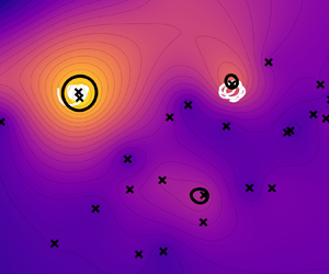
Figure 6. Comparison for the AVISO data between objective rotational sparse data diagnostic ${\mathrm {r}\alpha }$, $\mathrm {r}\alpha _{{ref}}$ and its quasi-objective single-trajectory counterpart $\overline {\mathrm {TRA}}$ under varying trajectory densities ($10 \ell ^{-2}, 1 \ell ^{-2}, 0.1 \ell ^{-2}$). The white markers denote the trajectory endpoints.

At a trajectory concentration of $10\ell ^{-2}$, $\overline {\mathrm {TRA}}$ (figure 6a) and ${\mathrm {r}\alpha }$ (figure 6d) appear qualitatively similar, with both suggesting relatively high rotation in the Gulf Stream meanders, and three distinct elliptic rotational maxima aligned with the eddy boundaries. For a trajectory density of $1 \ell ^{-2}$, ${\mathrm {r}\alpha }$ (figure 6e) is qualitatively indistinguishable from $\overline {\mathrm {TRA}}$ (figure 6b) with two of the three mesoscale LAVD eddies still visible as local maxima in both diagnostic fields. For this region of the ocean, we often have ocean drifter observations [e.g. Global Drifter Program (GDP)] at concentrations between $1 \ell ^{-2}$ and $0.1 \ell ^{-2}$, as discussed in § 3.2.1.

As we pass the extremely sparse sampling threshold to $0.1 \ell ^{-2}$, the leftmost eddy is still identifiable as a $\overline {\mathrm {TRA}}$ and ${\mathrm {r}\alpha }$ maximum (figures 6c and 6f, respectively) due to the presence of the single trajectory originating inside its boundary (white cross). The remaining eddies are no longer visible for either metric due to a lack of data, but $\overline {\mathrm {TRA}}$ still highlights a relatively higher rotation in the Gulf Stream. The local maximum $\overline {\mathrm {TRA}}$ within the dashed white box may be classified incorrectly as an eddy, but it actually corresponds to a region of high material rotation induced by shear in the Gulf Stream. In contrast, ${\mathrm {r}\alpha }$ has created multiple local maxima near the coast of Nova Scotia not present at higher concentrations.

At this extremely sparse resolution, we again replace $\boldsymbol {\bar {\omega }}(t)$, $\boldsymbol {\bar {v}}(t)$, and $\boldsymbol {\bar {x}}(t)$ with their time-averaged steady approximations, $\boldsymbol {v}_{{ref}}, \boldsymbol {\omega }_{{ref}}, \boldsymbol {x}_{{ref}}$ from (2.17)–(2.19). As with the Bickley jet statistics, this improves the accuracy of ${\mathrm {r}\alpha }$ with ${\mathrm {r}\alpha }_{{ref}}$ displayed in figure 6(i). With the steady reference frame, ${\mathrm {r}\alpha }_{{ref}}$ and $\overline {\mathrm {TRA}}$ again show nearly indistinguishable flow topologies. The coastal local maxima disappear, and the local maximum appears in the shear dominated meanders of the Gulf Stream. Furthermore, if we apply this steady reference frame change to higher concentrations (figure 6g and h), we obtain flow structure visualisations comparable to ${\mathrm {r}\alpha }$. This suggests that obtaining meaningful results using the extremely sparse steady reference-frame approach is resilient over a range of concentrations.

This effect stems from the effect of undersampling on bulk rotation and translation estimates. In figure 7, we display the $\boldsymbol {\bar {\omega }}(t)$ and $\boldsymbol {\bar {v}}(t)$ estimates for each trajectory concentration. At $100 \ell ^{-2}$ the mean flow properties are nearly constant over 15 days. This is consistent with the expectation from earlier studies that Eulerian features do not change significantly over such relatively small time scales in the ocean. As we progressively reduce the trajectory density, however, $\boldsymbol {\bar {\omega }}(t)$ and $\boldsymbol {\bar {v}}(t)$ start displaying strong oscillations in time. At extremely low trajectory densities ($<1 \ell ^{-2}$), the spatial averages are no longer representative of the underlying mean flow properties (dashed red curves in figure 7). These oscillations contribute unphysical fluctuations in the direction of $\boldsymbol {v}_{d}$ and hinder our ability to measure rotation with ${\mathrm {r}\alpha }$.

Figure 7. Data-based estimates for bulk translation velocity $|\boldsymbol {\bar {v}}(t)|$ and rotation $\boldsymbol {\bar {\omega }}(t)$ under varying trajectory density ($100 \ell ^{-2}, 10 \ell ^{-2}, 1 \ell ^{-2}, 0.1 \ell ^{-2}$).

To further quantify the impact of sparse sampling on ${\mathrm {r}\alpha }$, we repeat the $R^2$ distribution analysis that was performed for the unsteady Bickley jet. Using AVISO surface current data to generate an initial baseline at $100\ell ^{-2}$, we run $10^4$ random subsamplings at a range of concentration levels. The summary statistics of this experiment can be found in table 3. A consistent decrease in the $R^2$ mean, and increase in $R^2$ standard deviation is found as the data concentration levels decrease, though the level of ${\mathrm {r}\alpha }$ accuracy remains quite high. Even at a low concentration level of $1\ell ^{-2}$, we obtain a mean $R^2$ value of 0.92.

Table 3. Downsampling effect on ${\mathrm {r}\alpha }$ accuracy for AVISO Gulf Stream surface currents. Mean and standard deviation of $R^2$ values relating downsampled ${\mathrm {r}\alpha }$ with full-resolution calculations for $10^4$ random subsamplings at each resolution. Raw ${\mathrm {r}\alpha }$ values maintain a strong correlation until the extremely sparse threshold $(1 \ell ^{-2})$, at which point time-averaged reference values (ref) allow for a significant improvement in accuracy again.

The most precipitous drop in ${\mathrm {r}\alpha }$ accuracy is found from $1\ell ^{-2}$ to $0.1\ell ^{-2}$. One such example of this poor performance was highlighted in figure 6. We further validate the improvement in ${\mathrm {r}\alpha }$ accuracy at this extreme sparsity level in the last two columns of table 3. After transitioning to time-averaged reference frame values, there is a significant increase in accuracy, with the mean of $R^2$ jumping from 0.92 to 0.95 for $1\ell ^{-2}$, and from 0.45 to 0.89 for $0.1\ell ^{-2}$. With this simple reference-frame methodology we find $r\alpha$ is a promising Lagrangian flow rotation diagnostic for extremely sparse data.

3.1.3. Stationary concentrated vortex

Our third example considers the identification of elliptic coherent structures inside the stationary concentrated vortex model (SCVM) of Onishchenko et al. (2021). The SCVM represents finite-size cyclones in the Earth's atmosphere as steady axially symmetric solutions to the Euler equations. Both the vertical and radial extent of the vortex is controlled by model parameters. The SCVM fundamentally differs from the previous flows as it is a highly rotational flow with no bulk translation. Our investigation of the SCVM helps confirm that ${\mathrm {r}\alpha }$ and ${\rm r}\overline {\mathrm {TSE}}$ are robust diagnostics for approximating the shape and location of LCS and are not tailored to a specific kind of flow experiment (e.g. both high and low swirl number; Gupta, Lilley & Syred 1984).

The SCVM consists of inner and outer regions, an internal upwards motion and external downwards motion. A distinct central torus was also identified by Aksamit (2023) as a LCS. The cyclone is further divided vertically into a centripetal and centrifugal flow with upward-moving fluid recirculated from the top of the vortex back down.

The SCVM was originally derived as an axisymmetric flow from a stream function $\varPsi (r,v)$ and can be written in cylindrical coordinates as

(3.5)\begin{gather} \mathrm{v}_r ={-}\mathrm{v}_0 \frac{r}{L} \left( 1-\frac{z}{L} \right)\exp\left({-\frac{z}{L}-\frac{r^2}{r_0^2}}\right), \end{gather}

(3.6)\begin{gather}\mathrm{v}_\theta ={\pm} \mathrm{v}_{\theta_0}\frac{z}{L}\exp\left({-\frac{z}{L}-\frac{r^2}{r_0^2}}\right), \end{gather}

(3.7)\begin{gather}\mathrm{v}_z = 2\mathrm{v}_0 \frac{z}{L} \left( 1-\frac{r^2}{r_0^2} \right)\exp\left({-\frac{z}{L}-\frac{r^2}{r_0^2}}\right), \end{gather}

where $r_0$ is the radial extent separating inner and outer vortex structures, $L$ is the height of maximum vertical velocity at $r=0$ and $\mathrm {v}_0$ and $\mathrm {v}_{\theta _0}$ are characteristic velocities. For our example, we use $\mathrm {v}_0 = 1$, $L = 10$, $r_0 = 1$ and $\mathrm {v}_{\theta _0}=9$. We consider our characteristic length of the flow to be equal to the separation of inner and outer motions, $\ell =r_0=1$, and the approximate radius of the main central torus.

In figure 8 we compare the objective rotational diagnostics ${\mathrm {r}\alpha }$ and $\mathrm {LAVD}$ advected for $\Delta t = 500$ with the vorticity magnitude, $|\boldsymbol {\omega }|$ and the widely used lambda-2 criterion of Jeong & Hussain (1995). If $\boldsymbol {J}$ is the velocity gradient tensor, and $\boldsymbol {S}$ and $\boldsymbol {\varOmega }$ are the symmetric and antisymmetric parts, the lambda-2 criterion of Jeong & Hussain (1995) suggests that regions with negative intermediate eigenvalues of $\boldsymbol {S}^2 + \boldsymbol {\varOmega }^2$ (labelled $\lambda _2$) are part of a vortex core. Stationarity of the flow suggests $\overline {\mathrm {TRA}}$ would also be a suitable comparison, but in light of the strong performance of $r\alpha$ against $\overline {\mathrm {TRA}}$ in the previous two examples, we have left it out for compactness of presentation.

Figure 8. Comparison of rotation diagnostics ${\mathrm {r}\alpha }$, $\mathrm {LAVD}$, $\lambda _2$ and $|\boldsymbol {\omega }|$ for the SCVM in the $y=0$ plane. White contour lines are contours of the SCVM stream function $\varPsi$, indicating circulation patterns in the model. Note the agreement between ${\mathrm {r}\alpha }$, $\mathrm {LAVD}$, ${\rm r}\overline {\mathrm {TSE}}$ and $\mathrm {FTLE}$ features with the stream function structures, and the dissimilarity of $|\boldsymbol {\omega }|$ and $\lambda _2$ features.

From initial high spatial resolution ($2000\ell ^{-3}$) calculations, a 2-D slice along the $y=0$ plane is shown for each field in figure 8. We overlay these plots with the level-set contours of the SCVM stream function $\varPsi (r,v)$. As this is a stationary axisymmetric flow, $\varPsi$-contours provide us a ground truth of transport barrier structure. A qualitative contour comparison of the sparse metrics (${\mathrm {r}\alpha }$ and ${\rm r}\overline {\mathrm {TSE}}$) with $\varPsi$ show a comparable level of structure agreement as one can find from LAVD and FTLE structures. We find that ${\mathrm {r}\alpha }$ and $\mathrm {LAVD}$ contours suggest very similar rotational behaviour, with both indicating the same location of a central torus vortex surrounded by recirculating flow. Both r$\overline {\mathrm {TSE}}$ and FTLE show strong spiraling into the centre of the vortices identified by ${\mathrm {r}\alpha }$ and $\mathrm {LAVD}$. One notable difference between sparse and spatial-gradient-reliant diagnostics exists in the centre of the toroidal vortex core in ${\rm r}\overline {\mathrm {TSE}}$ which again have unnaturally low values when compared with FTLE, as we also saw in the unsteady Bickley jet.

We see a stark difference, however, when comparing $\varPsi$ with $|\boldsymbol {\omega }|$ and $\lambda _2$ fields. Contours of $|\boldsymbol {\omega }|$ and $\lambda _2$ are often orthogonal to $\varPsi$-contours, suggesting a disagreement in structure identification. We further investigate these qualitative findings by testing the ability of our rotation diagnostics to identify the dominant elliptic coherent structures in this vortex flow. Potential vortex boundaries are identified as the set of outermost closed convex contours for ${\mathrm {r}\alpha }$, LAVD and $|\boldsymbol {\omega }|$. Following the derivation of the $\lambda _2$ criterion, we use $\lambda _2<0$ as the designation of strong rotational motion (Jeong & Hussain 1995). Fluid parcels from inside the boundaries of these features are then advected for twice the integration time used for the Lagrangian diagnostics, $\Delta t = 1000$. This approach allows us to test both the Lagrangian and Eulerian diagnostics to identify features that maintain their coherence beyond the time horizon of data used for the initial boundary calculation.

These fluid particle paths are shown in figure 9 with trajectories coloured by the initial diagnostic field value. We include the corresponding figure 8 diagnostic field on the $y=0$ plane as a reference. The vortex core identified by ${\mathrm {r}\alpha }$ and $\mathrm {LAVD}$ maintain coherence over time, with seemingly no deviation of fluid from the domain identified as the central torus vortex (figure 9a,b). Given that ${\mathrm {r}\alpha }$ does not rely on the same 3-D velocity gradient data as $\mathrm {LAVD}$, ${\mathrm {r}\alpha }$ shows exceptional performance in identifying this LCS. Fluid initially inside $\lambda _2$ and $|\boldsymbol {\omega }|$ structures have instead maintained no coherence, and are sufficiently dispersed in the flow. The high $|\boldsymbol {\omega }|$ (figure 9d) fluid parcels are now mixed throughout the entire inner SCVM ‘beehive’ domain, inhabiting regions with both high and low $|\boldsymbol {\omega }|$ values. The $\lambda _2\!<\!0$ fluid is recirculating in both the inner and outer regions of the SCVM (figure 9c), with the $\lambda _2$-estimated vortex core parcels inhabiting the domain of both negative and positive $\lambda _2$ values. This is distinct from LAVD and ${\mathrm {r}\alpha }$ vortex trajectories that stay confined to the regions of high LAVD and ${\mathrm {r}\alpha }$, respectively.

Figure 9. Trajectories corresponding to coherent structures identified by the four diagnostics, calculated for the same integration times.

The ability of ${\mathrm {r}\alpha }$ to identify these same LCS at increasing sparsity is shown in figure 10. As our only 3-D numerical example, we utilise a random set of initial particle trajectories in three dimensions and extract isosurfaces from a reconstructed ${\mathrm {r}\alpha }$ field using natural neighbour interpolation. We utilise the same ${\mathrm {r}\alpha }$ value for 3-D level-set extraction as the outermost closed convex contour used to test vortex boundaries (figure 9). Plots of reconstructed ${\mathrm {r}\alpha }$ fields on the $y=0$ plane (figure 10a–c) reveal that small deviations from this range would not significantly change the topology of the surfaces in figure 10(d–f). Note the difference of $z$-value ranges between figures 10(a–c) and 10(d–f).

Figure 10. (a–c) Values of ${\mathrm {r}\alpha }_0^{500}$ on the $y=0$ plane reconstructed from randomly selected trajectories at decreasing particle density. The inner vortex is extracted at each concentration as the closed contours corresponding to the level-set value from figure 8. (d–f) Comparison of the inner vortex surface in ${\mathrm {r}\alpha }_0^{500}$ fields reconstructed from randomly selected trajectories at decreasing particle density. The inner vortex is extracted in each scenario as closed contours corresponding to the outermost closed convex contour in figure 9.

In figure 10, ${\mathrm {r}\alpha }$ at $10\ell ^{-3}$ looks only moderately different from $2000\ell ^{-3}$. Two distinct intersections of the central torus with the $y=0$ plane are still evident in white, and the annular shape is clearly visible in the associated isosurface. At $1\ell ^{-3}$, the ‘doughnut hole’ above $x=0$ becomes less obvious, but the horizontal and vertical extent of the central torus is still accurate. For $0.1\ell ^{-3}$, we use ((2.17)–(2.18)) to implement the same bulk time-averaged reference values for $\boldsymbol {v}_{{ref}}, \boldsymbol {\omega }_{{ref}}, \boldsymbol {x}_{{ref}}$. At this extremely sparse sampling, the correct extent of strong central rotation is still evident, as is a suggestion of the inner beehive feature, but the vortex surface is now sufficiently deformed that it no long resembles a torus.

3.2. Experimental data

In the previous section we investigated the ability of ${\mathrm {r}\alpha }$ and ${\rm r}\overline {\mathrm {TSE}}$ to accurately represent elliptic and hyperbolic LCS at increasing sparsity in numerical data. In this section, we show how the sparse capabilities of ${\mathrm {r}\alpha }$ apply to real experimental data for a 2-D and 3-D flow.

3.2.1. GDP database

For our first experimental data set we consider a set of drifters from the GDP (Lumpkin & Centurioni 2019) located in the North Atlantic Ocean. The GDP data set contains more than 40 000 drifters spanning the last four decades. Roughly 1200 drifters are currently active worldwide and report their position every 6 hours (Lumpkin & Pazos 2007).

Specifically, we focus here on a subset of drifters active over 15 days from 20 September to 4 October 2006 in the Gulf Stream (figure 11) during the same time period of analysis as in § 3.1.2. In figure 11, we reconstruct diagnostic fields from the true GDP tracks with a drifter density of $0.63 \ell ^{-2}$, for $\ell = 100\,\mathrm {km}$. We are thus in an extremely sparse data setting ($< 1 \ell ^{-2}$) and we again compute ${\mathrm {r}\alpha }$ by replacing the time-dependent mean flow properties with time-averaged $\boldsymbol {\omega }_{{ref}}, \boldsymbol {v}_{{ref}}$ and $\boldsymbol {x}_{{ref}}$ from the drifter data.

Figure 11. Drifter-based $\overline {\mathrm {TRA}}$ (a), ${\mathrm {r}\alpha }$ (b), $\overline {\mathrm {KE}}$ (c) and LAVD (d) in the North Atlantic Gulf Stream. The black crosses indicate drifter positions.

Following the sparse eddy identification study by Encinas-Bartos et al. (2022), we compare two sparse drifter-based rotation diagnostics, $\mathrm {r}\alpha _{{ref}}$ in figure 11(a) and $\overline {\mathrm {TRA}}$ in figure 11(b), with commonly used trajectory-averaged kinetic energy (KE; figure 11c) (e.g. Lumpkin 2016), and the full-resolution LAVD field using AVISO data from § 3.1.2. Though the AVISO current data may not be representative of the full spatial scale of flow features affecting the drifters, we include LAVD as a mesoscale comparison for general flow behaviour.

We do not compare with a direct ‘looping’ count as a user-defined threshold is inevitably required and differentiating between looping and non-looping trajectories is user-dependent and non-trivial (Encinas-Bartos et al. 2022). Instead, we extract looping segments for the reader to see from the drifter trajectories as proposed by the frame-dependent algorithm from Lumpkin (2016). The white trajectory segments indicate cyclonic loopers which frequently arise in connection with ocean eddies (see, e.g. Griffa, Lumpkin & Veneziani 2008; Dong et al. 2011). The full black curves in figure 11(a,b,d) denote the approximate vortex boundaries respectively obtained from drifter-based $\overline {\mathrm {TRA}}$ and ${\mathrm {r}\alpha }_{ref}$, and AVISO-based LAVD, respectively.

Both $\mathrm {r}\alpha _{{ref}}$ and $\overline {\mathrm {TRA}}$ are able to detect rotational features just to the south of the Gulf Stream from the extremely sparse GDP data. Cyclonic loopers are also observed in the regions surrounding the principal local maxima of $\mathrm {r}\alpha _{{ref}}$ and $\overline {\mathrm {TRA}}$. The leftmost eddy contains two looping drifters that display high rotational values (figure 11a,b). In contrast, $\overline {\mathrm {KE}}$ fails to clearly identify the leftmost eddy since it displays sharp gradients between the two drifters inside the eddy (figure 11c). Both $\mathrm {r}\alpha _{{ref}}$ and $\overline {\mathrm {TRA}}$ display a weaker rotational feature at roughly $32\,^{\circ }$N latitude and $64^{\circ }$W longitude. No loopers are identified in this region, but the yellow trajectories in the high ${\mathrm {r}\alpha }$ and $\overline {\mathrm {TRA}}$ zones show greater circulating behaviour with respect to the surrounding green trajectories (figure 11, bottom insets), suggesting stronger rotational motion in the surface currents. There is no feature that resembles any vortical structure in the $\overline {\mathrm {KE}}$ field in this region.

In this ocean buoy experiment, we were able to identify eddies adjacent to the Gulf Stream in both $\overline {\mathrm {TRA}}$ and ${\mathrm {r}\alpha }$ fields that were not identified using existing sparse data diagnostics. In contrast with the $\overline {\mathrm {TRA}}$, which requires additional assumptions on the frame of reference, the ${\mathrm {r}\alpha }$ returns structures that are valid for all observers. This suggests that ${\mathrm {r}\alpha }$ may be beneficial for systematic eddy analysis of the GDP data set that can complement remote-sensing based tools that lack submesoscale motion resolutions. In addition, ${\mathrm {r}\alpha }$ shows great promise as a buoy diagnostic for focused buoy deployments (e.g. LASER and GLAD) where buoy concentrations higher than $1\ell ^{-2}$ will result in more refined descriptions of the flow.

3.2.2. Large-scale LPT experiment

Our last example involves a novel, large-volume 3-D LPT velocimetry data set from an industrial-scale wind tunnel (Hou et al. 2021). Utilising glare-point spacing on large soap bubbles, Hou et al. (2021) were able to investigate the vortical wake behind a tractor–trailer model at a $9^{\circ }$ yaw angle. For details on the methodology, see Kaiser & Rival (2023). We compare two wind-tunnel experiments, one with the tractor–trailer model obstructing the flow, and a uniform flow without the tractor–trailer.

Each experiment provides around 300 s of trajectory data, sampled at 150 Hz with an average windspeed of 10 m s$^{-1}$. The bubble generator and camera setup produce time-varying particle concentrations at the very lower end of our computation spectrum. For measurements of the tractor–trailer wake, trajectory concentrations oscillate between 0.2 and 1.5$\ell ^{-3}$ with a mean concentration of 0.6$\ell ^{-3}$. The uniform flow measurements have a slightly higher resolution, ranging from 0.5 to 3$\ell ^{-3}$ and a mean concentration of 1.3$\ell ^{-3}$. To avoid significant oscillations in relative Lagrangian velocities, we again utilise the time-averaged reference frame determined by the bubble trajectories. Furthermore, as we are using trajectory data that quickly transits through the observation volume, we investigate 10-frame increments and require all trajectories to be present for every frame. At these extremely low concentrations, a single particle that disappears and reappears during the integration window may have a substantial effect on the deformation velocity of other fluid particles. A 10-frame integration time was chosen as a balance between the length of integration time and the number of tracks available to calculate meaningful mean values.

At the low trajectory concentration available in this turbulence experiment, meaningful time-resolved spatial derivatives are unattainable. Instead of relying on a spatial interpolant to visualise strong regions of rotation, we now demonstrate a complementary statistical approach using this sparse data set. In figure 12 we show the discrete probability histograms for common LPT flow diagnostics in addition to ${\mathrm {r}\alpha }$ analysis. The distribution of the particle speed over the entire 300 s (figure 12b) shows a slight speed up of the flow for the trailer wake, but the bubble trajectories travel for a shorter distance on average (figure 12c). The fluctuating streamwise components of bubble velocities were also nearly identical for the two flows.

Figure 12. Comparison of discrete probability histograms of frame-dependent metrics for the truck wake vortex and object-free uniform flow experiments at $\sim 1\ell ^{-3}$.

Sensor development for large-scale LPT is still an active field of research. Given the uncertainty in signal noise from nascent methodologies, such as the glare-point method used to generate for these data, flow diagnostics that maintain their utility for unknown noise levels can help to expedite the development of large-scale measurement tools. With the available information from the industrial-scale wind tunnel, none of the diagnostics in figure 12(b–d) present a clear picture of the wake dynamics. In fact, $\boldsymbol {v}_x'$ cannot distinguish between the two flows.

To complement these approaches, we compute 10-frame ${\mathrm {r}\alpha }$ values beginning at every frame available. This gives us a distribution of ${\mathrm {r}\alpha }_t^{t+10}(\boldsymbol {x}_0)$ for a wide range of $t$ and $\boldsymbol {x}_0$. From a set of trajectories at each time $t$, we then calculate the median of ${\mathrm {r}\alpha }$ ($\widetilde {{\mathrm {r}\alpha }}$) to quantify the general behaviour of the flow in each time window. The discrete probability histogram of $\widetilde {{\mathrm {r}\alpha }}$ for the two flows is shown in figure 12(a). The empty tunnel data are concentrated around a low peak, suggesting a relatively uniform flow domain and an accumulation of small turbulent oscillations, but no major rotational features. In contrast, the trailer wake data are distinguished by a larger range of values, with a heavy tail towards considerable rotation and high peak $\widetilde {{\mathrm {r}\alpha }}$. The physical meaning of this data suggests a more complex flow, with a higher degree of rotation, in this case because of the vortical wake. Even at this low concentration, and with this experimental methodology, we are able to identify distinguished rotating features in the flow.

We can begin to distinguish the spatial features of the flow by analysing the long-time trends in ${\mathrm {r}\alpha }$. In figure 13 we project all initial particle locations to the $y$–$z$ plane, and bin them in a $100\times 100$ grid. We again calculate $\widetilde {{\mathrm {r}\alpha }}$ for each bin and plot this in figure 13(a,b). The trailer wake in figure 13(a) has high rotation near its centre, and relatively higher ${\mathrm {r}\alpha }$ distributed throughout the flow domain when compared with the quiescent centre and lower values in figure 13(b). We quantify the spatial dependence of rotation on flow geometry by binning ${\mathrm {r}\alpha }$ in 10 bins along the radial distance from the centre of the flow. We show this radial axis as a dot and line in figure 13(a,b). Again, the median ${\mathrm {r}\alpha }$ values from these bins shows the trailer wake generates a much greater degree of rotation on the fluid, starting from a minimum where little data are available, with a local maximum in the vortex core, then gradually increasing as we move away in the flow. At nearly every location, the empty tunnel generates limited fluid rotation with lower ${\mathrm {r}\alpha }$ values.

Figure 13. (a,b) Binned median value of ${\mathrm {r}\alpha }_0^t(\boldsymbol {x}_0)$ after projecting in the streamwise direction onto the $y$–$z$ plane. The trailer wake has high rotation in its core, and relatively higher $\widetilde {{\mathrm {r}\alpha }}_0^t$ values distributed across the flow. The empty tunnel, in contrast has a low rotational core, with higher $\widetilde {{\mathrm {r}\alpha }}_0^t$ appear only on the edges of the measurement domain. This is confirmed by binning the ${\mathrm {r}\alpha }_0^t$ values by radial distance from the flow centre, and calculating median values ($\widetilde {{\mathrm {r}\alpha }}_0^t(r)$, panel c). Note the radial centres and axes are marked by blue dots and lines in panels (a,b).

The results here provide a good baseline for experimental LPT data that were not designed with ${\mathrm {r}\alpha }$ analysis in mind. As future experiments may be designed that consider ${\mathrm {r}\alpha }$ requirements, further improvement on the identification and analysis of coherent rotational flow features is expected. Furthermore, given the connections between ${\mathrm {r}\alpha }$, curvature (e.g. § 2.4) and rotation times, concerted future effort may help connect classical notions of geometry, eddy turnover times, spectral analysis and sparse trajectory data in an objective manner, in addition to designating strongly and weakly rotating regions of a flow.

4. Conclusion and outlook

Objective coherent structure identification tools are important in a wide range of scientific and industrial fields. Methods that work equally well for gridded and sparse Lagrangian data allow meaningful comparisons between model and observations, and can provide new insights for experimental studies. In this work, we have mathematically derived new frame-independent diagnostics of trajectory rotation and stretching well-suited for coherent structure identification in sparse experimental trajectory data. Through multiple systematic comparisons with existing Lagrangian flow diagnostics, we have shown that:

1. (i) ${\rm r}\overline {\mathrm {TSE}}$ and ${\mathrm {r}\alpha }$ are objective metrics that can identify elliptic and hyperbolic LCS in highly unsteady flows, and that work equally well in flows with large or small bulk translation and rotation;

2. (ii) ${\rm r}\overline {\mathrm {TSE}}$ and ${\mathrm {r}\alpha }$ work well in many of the situations where the quasi-objective diagnostics $\overline {\mathrm {TSE}}$ and $\overline {\mathrm {TRA}}$ have previously been successful, including ocean drifter applications;

3. (iii) ${\mathrm {r}\alpha }$ can designate regions with locally strong rotation in 2-D and 3-D flows for extremely sparse data;

4. (iv) ${\mathrm {r}\alpha }$ values maintain accuracy and interpretability at extremely sparse sampling; and

5. (v) ${\rm r}\overline {\mathrm {TSE}}$ and ${\mathrm {r}\alpha }$ provide an avenue for meaningful LPT analysis and post-processing that does not require assumptions of steady-state flows or data interpolation to an Eulerian grid.

To assist future practitioners, we have also developed two guidelines based on the results of the present research and our experiences while conducting it.

1. (i) If the trajectory concentration is below one $\ell ^{-2}$ or $\ell ^{-3}$, we recommend using time-averaged values of the experiment-derived $\bar {\boldsymbol {v}}$, $\bar {\boldsymbol{\omega} }$ and $\bar {\boldsymbol {x}}$

2. (ii) As the trajectory concentration decreases, the continuity of individual trajectory data becomes more important as each data point contributes more to spatial averages. It is then beneficial to select observation windows or trajectory sets for which trajectories are continuously present to prevent unphysical fluctuations in $\boldsymbol {v}_d$ caused by intermittent trajectory data.

Being able to identify coherent flow features, or at least local stretching and rotation rates, using ${\rm r}\overline {\mathrm {TSE}}$ and ${\mathrm {r}\alpha }$ for the analysis of unsteady flows in a physically meaningful, frame-indifferent manner will help advance our study of fluid dynamics in large and natural domains. Further applications of these methods, such as the time-series analytic techniques used by Aksamit et al. (2023), is expected to open the door for an even wider range of experiments over a vast range of scales that can harness the Lagrangian nature of turbulent structures.