Mapping interacting QTL for count phenotypes using hierarchical Poisson and binomial models: an application to reproductive traits in mice

Summary

We proposed hierarchical Poisson and binomial models for mapping multiple interacting quantitative trait loci (QTLs) for count traits in experimental crosses. We applied our methods to two counted reproductive traits, live fetuses (LF) and dead fetuses (DF) at 17 days gestation, in an F₂ female mouse population. We treated observed number of corpora lutea (ovulation rate) as the baseline and the total trials in our Poisson and binomial models, respectively. We detected more than 10 QTLs for LF and DF, most having epistatic and pleiotropic effects. The epistatic effects were larger, involved more QTLs, and explained a larger proportion of phenotypic variance than the main effects. Our analyses revealed a complex network of multiple interacting QTLs for the reproductive traits, and increase our understanding of the genetic architecture of reproductive characters. The proposed statistical models and methods provide valuable tools for detecting multiple interacting QTLs for complex count phenotypes.

1. Introduction

Reproductive traits of animals determine the efficiency of food production, and hence are economically important traits for genetic improvement in the livestock industry (Rocha et al., 2004b). However, since the reproductive traits usually have a low heritability, their improvement has met with limited success (Hansen et al., 1983; Avalos & Smith, 1987; Bennett & Leymaster, 1989; Lamberson, 1990). Fortunately, along with the recent advances of genomic technologies and the collective efforts of statistical genetics, methodologies have been introduced to identify quantitative trait loci (QTLs) regulating reproductive traits, and ultimately enhance genetic processes by using QTL-complemented breeding and selection strategies in animal food production (Rathje et al., 1997; Rohrer et al., 1999; Wilkie et al., 1999; Cassady et al., 2001; King et al., 2003; Holl et al., 2004; Rocha et al., 2004b).

Most QTL mapping studies for counted reproductive traits have used interval mapping or composite interval mapping, which focus on detecting marginal (main) effects of QTL (Kirkpatrick et al., 1998; Spearow et al., 1999; Rocha et al., 2004 b; Sato et al., 2006; Ren et al., 2009). Epistatic interaction effects (epistasis) have not been thoroughly examined, even though the genetic architecture of most quantitative traits in organisms from plants to animals including humans is quite complex, including inputs from multiple QTLs and epistasis (Doebley & Stec, 1991; Cheverund & Routman, 1995; Lynch & Walsh, 1998; Price & Courtois, 1999; Sugiyama et al., 2001; Wade, 2001; Kopp et al., 2003; Carlborg & Haley, 2004). Furthermore, some studies have shown that epistatically acting QTLs play a larger role than do the marginal effect QTLs in genetic modulation and evolution of quantitative traits (Yu et al., 1997; Yi et al., 2004a, b, 2006; Moore, 2005; Valdar et al., 2006). Therefore, to better understand the genetic architecture of counted reproductive traits, statistical analyses are required to simultaneously identify main effects and epistatic interactions of multiple QTLs.

Yi & Banerjee (2009) proposed a unified methodology for mapping multiple interacting QTLs based upon the hierarchical generalized linear model framework. The key to the approach is the use of a continuous prior distribution on coefficients that favours sparseness in the fitted models and facilitates computation. The method of Yi & Banerjee (2009) can analyse various continuous and discrete phenotypes, and can fit a large number of effects, including covariates, main effects of numerous loci and epistatic and gene–environment interactions. Yi & Banerjee (2009) illustrated the hierarchical generalized linear model framework with normal and probit models for continuous and binary traits. In this study, we developed hierarchical Poisson and binomial models for mapping multiple interacting QTLs for complex count traits in experimental crosses based on the approach of Yi & Banerjee (2009).

We applied our methods to data collected from a QTL mapping study of female reproductive traits in mice (Rocha et al., 2004a, b). The mouse sample was derived from parental lines having undergone long-term selection for high and low body weight gain. The previous analysis of these mouse data adopted the composite interval mapping method and detected 15 QTLs on five chromosomes for six reproductive traits. However, epistatic effects on the traits were not evaluated. In addition, two discrete counted reproductive traits, live fetuses (LF) and dead fetuses (DF), were treated as continuous traits. Improved models for these two count phenotypes should be Poisson models with observed number of corpora lutea (ovulation rate (OR)) treated as the baseline or offset, or binomial models treating LF and DF as the numbers of ‘success’ out of the corresponding number of corpora lutea (trials). The observed number of OR provides us the information about the upper bound of LF and DF. Therefore, to comprehensively and properly explore the genetic architecture of these reproductive traits in mice, we reanalysed the data by using the hierarchical Poisson and the binomial regression models. The aims of the present study were to estimate the epistatic effects of interacting QTLs on reproductive traits, and to detect possible additional QTLs for these traits.

2. Materials and methods

The mouse population, phenotypes and marker genotyping have been presented in detail in Rocha et al. (2004a, b), but are briefly described here.

(i) Mouse lines and crosses

A total of 439 F₂ female mice were bred from two long-term selected lines, the high-growth M16i line and the low-body-weight L6 line. The former was derived from an outbred population, whereas the latter was derived from a cross of four inbred lines. M16i females were intercrossed with L6 males, and the resulting F₁ mice were inter se mated (no full-sib pairings) in two consecutive replicates encompassing a total of 64 full-sib F₂ families. These mice were reared at 21°C in a 12:12 h light:dark cycle and 55% relative humidity. Food and water were supplied ad libitum. All the animals were handled according to the Institutional Animal Care and Use Committee Guidelines.

(ii) Phenotypes and environmental effects

To measure the reproductive traits of female mice, 10-week-old F₂ females were exposed to unrelated F₁ males (B6C3F1/J) until a copulatory plug was detected. Pregnant females were subsequently euthanized at day 17 of gestation to obtain three counted reproductive phenotypes: LF, DF and OR (also called corpora lutea) (Fig. 1). Body weights at 10 weeks of age (WK10) were also measured, which are significantly correlated with the reproductive phenotypes (Rocha et al., 2004b). Thus, our models adjusted for the covariates WK10 as well as the family indicator as environmental factors.

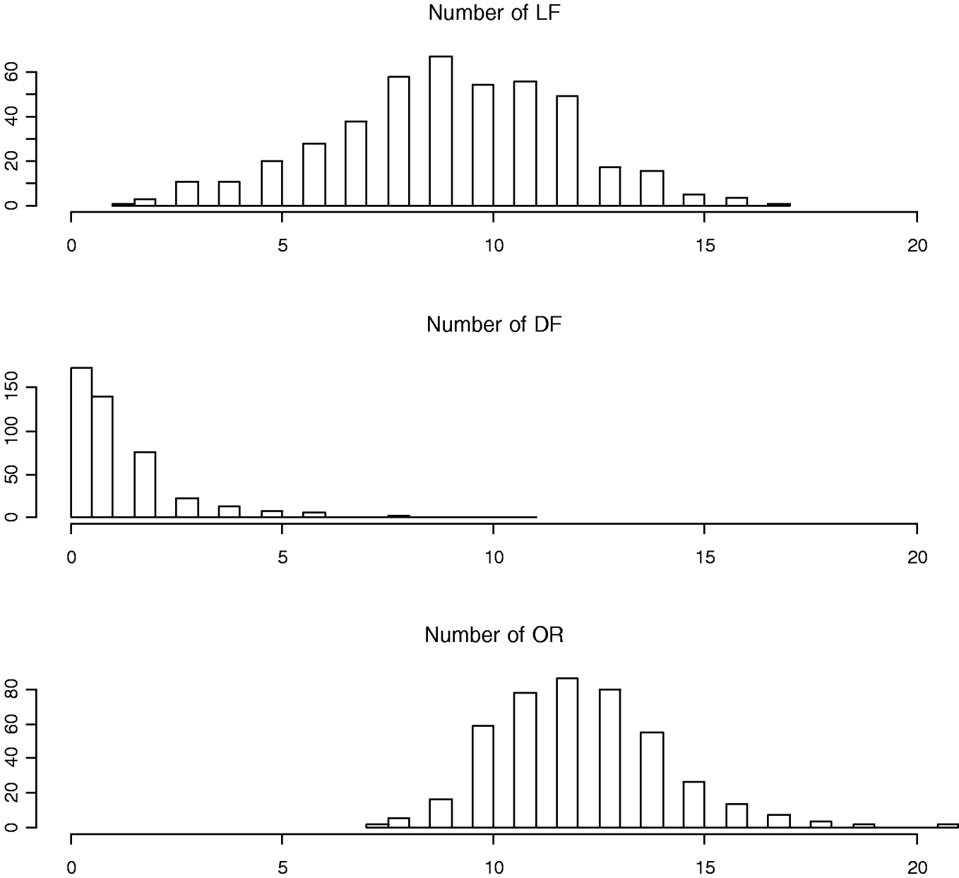
Fig. 1. Histograms of numbers of LF, DF and OR (also called corpora lutea).

(iii) Genotyping

A total of 63 fully informative microsatellite markers spanning the 19 autosomes were genotyped (Rocha et al., 2004a, b). Marker genotypes were determined by PCR and agarose gel electrophoresis protocols. Segregation distortion was evaluated by Chi-square test. Detection and correction of genotyping errors were conducted with MAPMAKER. A linkage map was generated with MAPMAKER/EXP and QTL analysis was carried out after marker distances were estimated. The marker linkage map covered 1257·8 cM (Kosambi) with an average spacing of 30 cM. A total of 21 (0·04%) marker genotypes were missing.

(iv) Statistical analyses

(a) Hierarchical Poisson and binomial models

Poisson and binomial models were used to detect QTL for the numbers of LF and DF. The Poisson model treated the number of LF and DF as counted responses relative to the number of OR, and the binomial model treated the number of LF and DF as the events of ‘success’ out of the corresponding ‘trials’ (the number of OR). Under each of these models, two approaches were applied: the first considering only main effects of QTL, and the second considering not only main effects but also their epistatic effects. All the models included WK10 and the family indicator as continuous and categorical covariates, respectively.

Denoting the number of LF or DF by y_i and the number of OR by T_i, for mouse i=1, …, n, the Poisson epistatic QTL model can be expressed as

(1)

and the binomial epistatic QTL model can take the form

(2)

where Poisson(T_iθ_i) presents Poisson distribution with mean T_iθ_i, and Bin(T_i,p_i) represents binomial distribution with size T_i and probability p_i; X _E, X _G and X_GG are design matrices for the environmental effects, main effects (additive and dominance) and epistatic effects (additive–additive, additive–dominance, dominance–additive and dominance–dominance), respectively; β₀ is the intercept, and β_E, β_G and β_GG are vectors of the environmental, main and epistatic effects, respectively. In the Poisson model, θ_i is the underlying rate per unit of OR for the ith mouse, and the logarithm of θ_i is expressed as a linear predictor of the environmental effects, main and epistatic effects of potential QTL. In the binomial model, p_i is the probability of each OR being live or dead for the ith mouse, and the logit transformation is used to relate p_i to the environmental effects, main and epistatic effects of potential QTLs. The Poisson and binomial models are different but both reasonable for the present data analyses. It would be expected that these two models may each enable us to detect some different QTLs.

The genetic variables were coded by using a modified Cockerham genetic model (Yi & Banerjee, 2009). The dominance variable was coded as −0·5 and 0·5 for homozygotes and heterozygote of each QTL, respectively. To achieve the same scale as that of the dominance contrast, the additive variable was coded as −2^−0·5, 0 and 2^−0·5 for the three genotypes of F₂ population, rather than the original Cockerham codes of −1, 0 and 1. The epistasis X_GG was constructed by multiplying two corresponding main-effect variables. For each environmental variable, the raw values were transformed to have a mean of 0 and a standard deviation of 0·5 (Gelman et al., 2008; Yi & Banerjee, 2009). This transformation standardized all the environmental effects to the scale of all the genetic main effects described above. For loci with missing genotypic values, the codes of contrasts were replaced by their conditional expectations given the observed marker data (Haley & Knott, 1992). Although the proposed models can include loci between the observed markers, we describe our methods by considering observed markers as potential QTLs (e.g. Xu, 2007; Yi & Banerjee, 2009).

A total of 63 observed markers lead to a total of 7938 effects, including 63 additive effects, 63 dominance effects and 7812 epistatic effects. Most of these effects are expected to be zero or at least negligible. To incorporate this notion into the model and to make the large-scale model identifiable, an independent Student-t prior was assumed on coefficients β_j for j=1, …, J (Yi & Banerjee, 2009). For the intercept β₀, a weakly informative prior with ν₀=1 and s ₀=10 was used, and for main and epistatic effects, ν_j=0·01 and s_j=10⁻⁴ were assigned. These shrinkage priors give each coefficient a high probability of being near zero while still allowing for occasionally large effects (Yi & Xu, 2008; Yi & Banerjee, 2009). To facilitate the estimation of parameters, the t distribution was expressed as a mixture of normal distributions with mean 0 and variance distributed as scaled inverse-χ²:

(3)

(b) Model fit and search algorithm

The computational algorithm of Yi & Banerjee (2009) as implemented in the freely available R package qtlbim (Yandell et al., 2007) was used to fit the Poisson and binomial models by estimating the posterior modes of the coefficients. Yi & Banerjee (2009) developed a procedure to fit generalized linear models with the Student-t prior by incorporating an expectation–maximum (EM) algorithm into the usual iteratively weighted least squares (IWLS). The IWLS algorithm approximates the generalized linear model by a weighted normal linear regression (Gelman et al., 2003). At each iteration, one calculates pseudo-datum z_i and pseudo-variance σ_i ² for each observation i based on the current estimates of parameters, approximates the generalized linear model likelihood p(y_i| X_iβ,φ) by the normal likelihood N(z_i| X_iβ,σ_i ²), and then updates the parameters β_j by a weighted linear regression. The EM algorithm of Yi & Banerjee (2009) treats variances τ_j ² as missing data and replaces them by their posterior means at each E-step. Given the variances τ_j ², the parameters β_j are estimated by including the priors of β_j|τ_j ²~N(0,τ_j ²) as additional ‘data points’ in the normal likelihood N(z_i| X_iβ,σ_i ²). Briefly, the algorithm starts with initial values for each τ_j ² and β_j, and then proceeds as follows: (1) based on the current values of β_j, calculate pseudo-datum z_i and pseudo-variance σ_i ²; (2) E-step: replace each variance τ_j ² by its conditional posterior expectation; (3) M-step: perform the weighted least square regression based on the normal likelihood approximation to obtain estimates and (4) repeat steps 1–3 until convergence.

The hierarchical model can simultaneously handle many correlated variables (Xu, 2007; Yi & Banerjee, 2009). However, fitting a model with thousands of variables requires large memory and intensive computation. Thus, the model search strategy proposed by Yi & Banerjee (2009) was used to build a parsimonious model. The approach sets two threshold values t ₁ (say 10⁻¹⁰) and t ₂ (say 0·005) to control the effect size and the P-values, respectively, and then proceeds to identify significant effects as follows: (1) searching for main effects: for each chromosome c (c=1, 2, …, 19), simultaneously add all possible main effects for markers on chromosome c into the current model, fit the model, and then delete main effects satisfying ; (2) searching for epistatic effects among the included main effects: simultaneously add all possible interactions among the included main effects into the current model, fit the model, and then delete epistatic effects satisfying ; (3) searching for epistatic effects between the excluded and the included main effects: for chromosome c (c=1, 2, …, 19), simultaneously add all possible interactions between the remaining main effects (not included in the current model) on chromosome c and the included main effects into the current model, fit the model, and then delete epistatic effects ; (4) removing main and epistatic effects with P-values larger than t ₂ from the current model.

After these steps, a final model would be obtained with both the preset environmental effects and the genetic effects that are associated with the phenotype. The estimates of these effects and the corresponding P-values indicate how strongly they influence the phenotype. We present estimate, standard error and P-value for each effect included in the final model, and calculated two measures of model fit and comparison, the deviance and the Akaike information criterion (AIC).

3. Results

(i) LF

(a) Poisson models

Using the main-effect model, five main effects were detected (the left panel of Fig. 2). Among them, two additive effects were located on chromosomes 2 and 10, and three dominance effects on chromosomes 1, 2 and 10, respectively. The strongest main effect on LF was on chromosome 2, at position 65·3 cM, and it accounted for the highest proportion of phenotypic variance (about 3%). The P-values for the main effects were all less than 0·05.

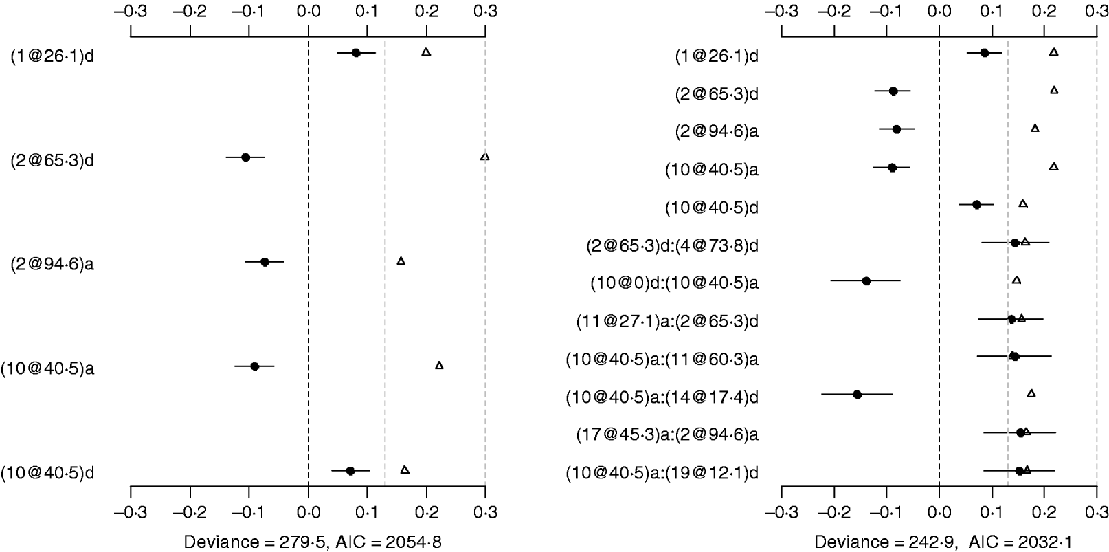
Fig. 2. Poisson main-effect (left) and epistatic (right) models for LF: estimated effects with±1 standard errors (dots and short lines), P-values (rescaled as −log₁₀p/10) (triangles), and deviance and AIC. The notation for additive effect (C@h)a dominance effect (C@h)d, indicates chromosome C and position h cM. The term X₁:X₂ represents interaction between X₁ and X₂. The two grey lines indicate the P-values of 0·05 and 0·001, respectively.

The Poisson epistatic model detected five main effects and seven epistatic effects (the right panel of Fig. 2). The five main effects were identical to those of the main effect model. Among the seven epistatic effects, there were two additive–additive, three additive–dominance, one dominance–additive and one dominance–dominance effects on LF located on some pairs of the seven chromosomes (2, 4, 10, 11, 14, 17 and 19). The epistatic effects involved three QTLs identified in the main effect model and seven novel QTLs, suggesting that the epistasis model can identify QTLs with weak main effects but strong epistasis. The strongest epistatic effect on LF was observed between chromosome 10 and chromosome 14. The absolute values of estimated epistatic effects ranged from 0·13 to 0·16, which were about two times greater than those of the main effects, and the total proportion of phenotypic variances explained by the epistatic effects was approximately 9%, which was higher than that of the main effects. This revealed evidence that QTL affect LF mainly through their epistatic effects and the epistasis plays a more important role than does the main effect in controlling the genetic variation of LF. The P-values for the main and epistatic effects were all less than 0·05.

For comparison purposes, the Poisson main-effect model for LF was refitted without model search (i.e. always including all of 126 additive and dominance effects in the model). Figure 3 shows that the main effects detected in this saturated model coincided with those in the parsimonious model (the left panel of Fig. 2). The majority of genetic effects were shrunk to zero, indicating that the proposed model with shrinkage prior can capture the notion that most genetic effects influencing LF are very weak. We also tried to simultaneously fit all the main effects and epistatic interactions, but the attempt failed because of requirement of large memory. This demonstrated that a model search strategy is necessary to build a parsimonious model by seeking significant genetic effects when the number of effects is huge.

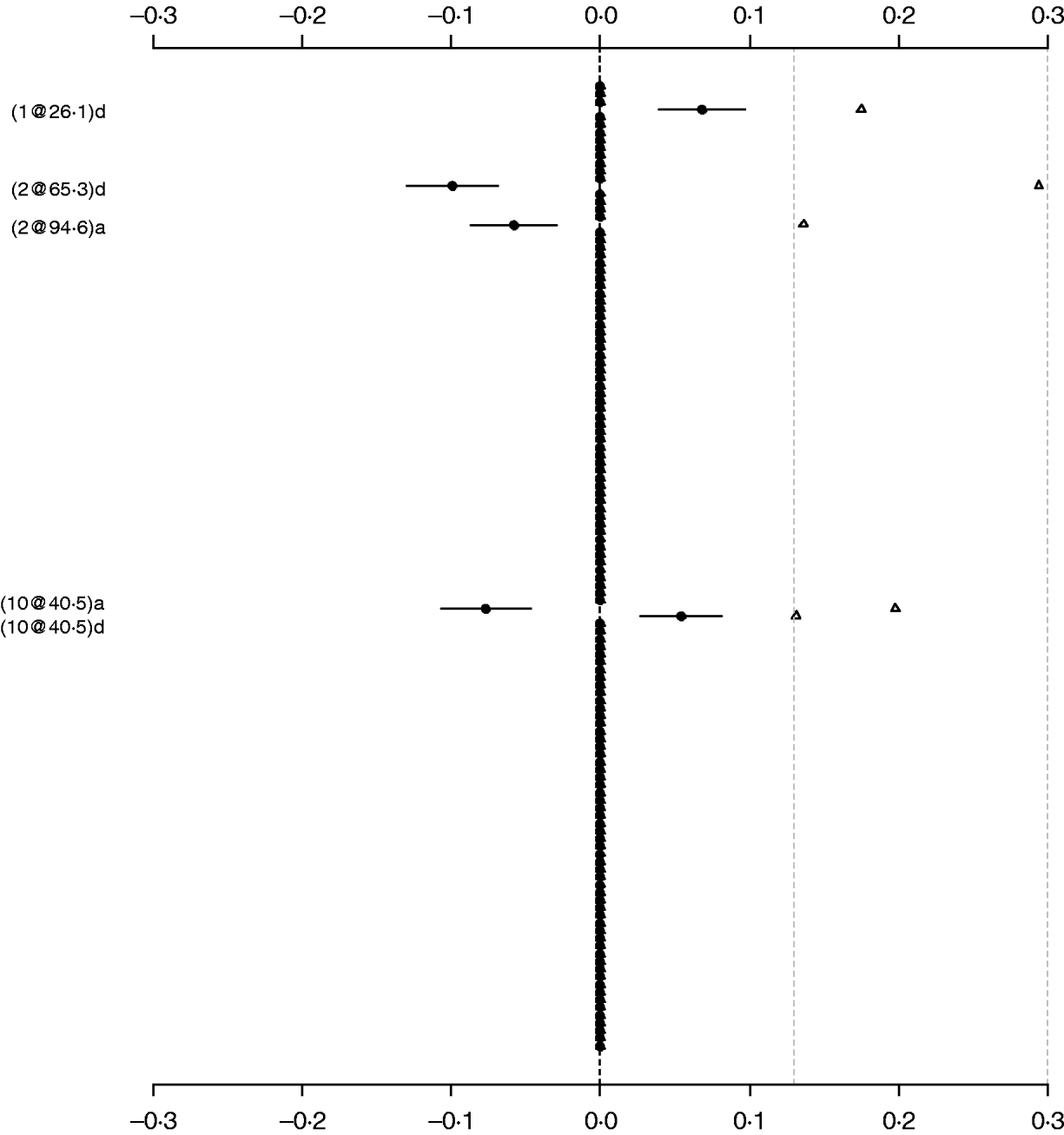
Fig. 3. Poisson main-effect model without model search for LF: estimated effects with±1 standard errors (dots and short lines), and P-values (rescaled as −log₁₀p/10) (triangles). The notation for additive effect (C@h)a dominance effect (C@h)d, indicates chromosome C and position h cM. The term X₁:X₂ represents interaction between X₁ and X₂. The two grey lines indicate the P-values of 0·05 and 0·001, respectively.

(b) Binomial models

The binomial main-effect model identified seven main effects (the left panel of Fig. 4). Among these main effects, four additive effects were located on chromosomes 2, 6 and 9, and three dominance effects on chromosomes 1, 2 and 10, respectively. The strongest main effect on LF was on chromosome 9, at position 0 cM, and it contributed the highest proportion (about 6%) to the phenotypic variance. The P-values for the main effects were all less than 0·0005.

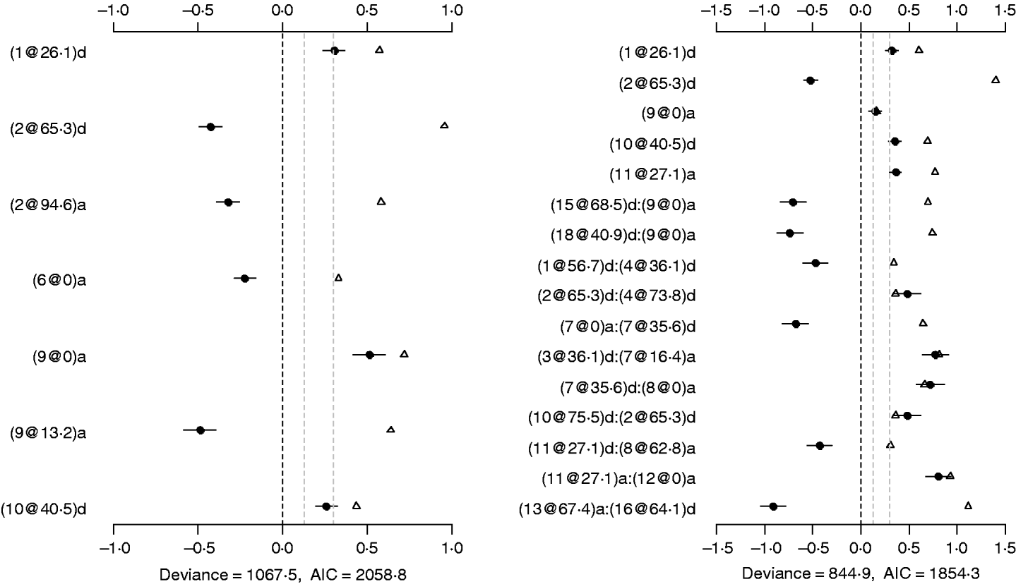
Fig. 4. Binomial main-effect (left) and epistatic (right) models for LF: estimated effects with ±1 standard errors (dots and short lines), P-values (rescaled as −log₁₀p/10) (triangles), and deviance and AIC. The notation for additive effect (C@h)a dominance effect (C@h)d, indicates chromosome C and position h cM. The term X₁:X₂ represents interaction between X₁ and X₂. The two grey lines indicate the P-values of 0·05 and 0·001, respectively.

Under the epistatic model, five main effects and 11 epistatic effects were identified (the left panel of Fig. 4). Among the five main effects, four effects overlapped those in the binomial main-effect model. The strongest main effect on LF was on chromosome 2, at position 65·3 cM, and it explained the highest proportion (about 5%) of phenotypic variance. Among the 11 epistatic effects, there were one additive–additive, two additive–dominance, five dominance–additive and three dominance–dominance effects. The epistatic effects involved three main effects that were identified and 16 effects that were not identified in the main-effect model. This shows that the model can identify QTLs which have a weak main effect but a strong interaction with other QTLs. The strongest epistatic effect was observed between chromosome 13 and chromosome 16. The absolute values of estimated epistatic effects ranged from 0·4 to 0·9, two times greater than those of main effects, and the total proportion of phenotypic variance explained by the epistatic effects was approximately 23%, about two times greater than that of main effects. All the P-values for the main and epistatic effects in the model were less than 0·001.

(ii) DF

(a) Poisson models

The Poisson main-effect model detected nine main effects on DF (the left panel of Fig. 5). Among these main effects, six additive effects were on chromosomes 1, 3, 6, 8, 10 and 11, and three dominance effects on chromosomes 1, 5 and 14, respectively. The strongest main effect on DF was on chromosome 6, at position 0 cM, and it contributed the highest proportion (about 2%) to the overall phenotypic variance. The P-values for the main effects were all less than 0·05.

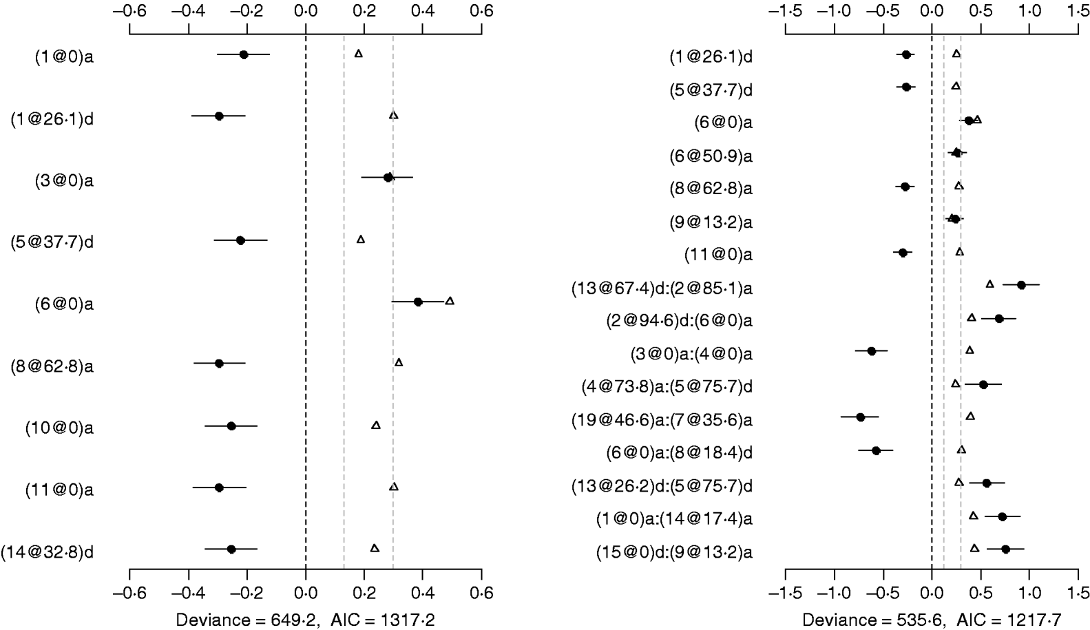
Fig. 5. Poisson main-effect (left) and epistatic (right) models for DF: estimated effects with ±1 standard errors (dots and short lines), P-values (rescaled as −log₁₀p/10) (triangles), and deviance and AIC. The notation for additive effect (C@h)a dominance effect (C@h)d, indicates chromosome C and position h cM. The term X₁:X₂ represents interaction between X₁ and X₂. The two grey lines indicate the P-values of 0·05 and 0·001, respectively.

Using the Poisson epistatic model, seven main effects and nine epistatic effects were identified (the right panel of Fig. 5). Among the seven main effects, five were identical to those identified in the main-effect model. The strongest main effect on DF was the same as that in the main-effect model. Among the nine epistatic effects, there were three additive–additive, two additive–dominance, three dominance–additive and one dominance–dominance effects. The epistatic effects involved only one main effect that was identified and 15 effects that were not identified in the main-effect model. The strongest epistatic effect on DF was observed between chromosome 2 and chromosome 13, accounting for the highest proportion of phenotypic variance (about 3%). The absolute values of estimated epistatic effects ranged from 0·5 to 0·9, which were about three times greater than those of main effects, and the total proportion of phenotypic variances explained by the epistatic effects was approximately 15%, about two times greater than that of main effects. The P-values for the main and epistatic effects were less than 0·001.

(b) Binomial models

The binomial main-effect model identified nine main effects (the left panel of Fig. 6). Seven additive effects were located on chromosomes 1, 3, 6, 8, 9, 10 and 11, and two dominance effects on chromosomes 14 and 18, respectively. The strongest main effect on DF was on chromosome 6, at position 0 cM, and it contributed the highest proportion (about 2%) to the phenotypic variance. The P-values for the main effects were all less than 0·01.

Fig. 6. Binomial main-effect (left) and epistatic (right) models for DF: estimated effects with ±1 standard errors (dots and short lines), P-values (rescaled as −log₁₀p/10) (triangles), and deviance and AIC. The notation for additive effect (C@h)a dominance effect (C@h)d, indicates chromosome C and position h cM. The term X₁:X₂ represents interaction between X₁ and X₂. The two grey lines indicate the P-values of 0·05 and 0·001, respectively.

The epistatic model detected seven main effects and ten epistatic effects (the right panel of Fig. 6). Among the seven main effects, five coincided with those identified in the binomial main-effect model. The strongest main effect on DF was located on chromosome 1, at position 26·1 cM, and it accounted for the highest proportion of phenotypic variance (about 2%). There were three additive–additive, three additive–dominance, three dominance–additive and one dominance–dominance effects on DF Among these epistatic effects, six were also identified by the preceding Poisson epistatic model for DF. The epistatic effects involved three main effects that were identified and 15 effects that were not identified in the main-effect model. The strongest epistatic effect on DF was between chromosome 2 and chromosome 6. The absolute values of estimated epistatic effects ranged from 0·6 to 1·0, which were about two times greater than those of main effects, and the total proportion of phenotypic variances explained by the epistatic effects was approximately 20%, two times greater than that of main effects. All the P-values for the main and epistatic effects in the model were less than 0·001.

(iii) Model comparison

We used two summary measures, the deviance and the AIC, to compare different models. The deviance, defined as −2 times the log-likelihood, is a statistical summary of model fit; lower deviance means better fit to data. The AIC, defined as deviance +2 (number of predictors), measures the predictive power; a model is estimated to reduce out-of-sample prediction error if the AIC decreases. In all the analyses, the epistatic model had lower deviance and AIC than the corresponding main-effect model (Figs 2–6). This indicated that inclusion of the significant epistatic interactions improved the fit of the model to data and reduced out-of-sample prediction error.

(iv) Treating discrete LF and DF as normally continuous traits

To investigate whether or not count phenotypes can be analysed by methods for continuous traits, we performed Bayesian methods by treating the count phenotypes LF and DF or the ratios LF/OR and DF/OR as normally continuous traits. We also tried to use the Box–Cox transformation to these traits and obtained similar results displayed here. Our analyses used the same priors and the model search method as in the analyses of our Poisson and Binomial models. Figure 7 displays the estimates, standard errors and P-values for the effects detected in the final models. Most of the effects detected by the normal models were also detected in the Poisson and the binomial models. However, the normal models missed several strong effects that were detected by both the Poisson and the Binomial models. The results indicated that the proposed methods were more appropriate for analysing the count phenotypes. This is expected from the general framework of generalized linear models (e.g. Gelman et al., 2003).

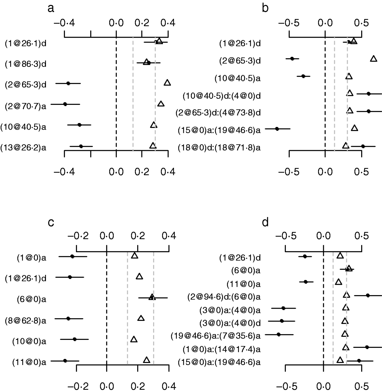
Fig. 7. Treating discrete LF and DF as normally continuous traits. a, main-effect model for LF; b, epistatic model for LF; c, main-effect model for DF; d, epistatic model for DF; estimated effects with ±1 standard errors (dots and short lines), P-values (rescaled as −log₁₀p/10) (triangles), and deviance and AIC. The notation for additive effect (C@h)a dominance effect (C@h)d, indicates chromosome C and position h cM. The term X₁:X₂ represents interaction between X₁ and X₂. The two grey lines indicate the P-values of 0·05 and 0·001, respectively.

4. Discussion

We have developed hierarchical Poisson and binomial models for mapping multiple interacting QTLs for count phenotypes based upon the unified generalized linear model framework of Yi & Banerjee (2009). Our method can fit a large number of effects, including covariates, main effects of numerous loci, and epistatic and gene–environment interactions, and can accommodate the correlation among the variables. Many complex traits, including reproductive phenotypes in mice, were measured as Poisson or binomial data. However, statistical methods for mapping multiple interacting QTLs for such phenotypes have not been fully developed previously.

To better characterize the genetic architecture of reproductive traits in mice, we applied our methods to two counted reproductive traits, LF and DF, in an F₂ female mouse population. Since the observed number of OR provides important information about the variation of LF and DF, the numbers of LF and DF were modelled using the Poisson model with OR as an offset, and as the events of ‘success’ out of total ‘trials’ (OR) using the binomial model. As described earlier, the Poisson and binomial models capture different properties of the trait, and allow us to detect some different QTLs. In contrast, since the Poisson distribution can be derived as a limiting case to the binomial distribution as the number of trials goes to infinity and the expected number of successes remains fixed, the two models can lead to similar results (Casella & Berger, 2001). In the present study, however, since the sample size (n=439) is not large enough and the proportions of LF and DF (0·75 and 0·10, respectively) are not small, it is not surprising that the QTLs detected in the Poisson models are not in full agreement with those detected in the binomial models. Furthermore, since the proportion of DF is lower than that of LF, there is more coincidence between two models for DF than that for LF.

More than 10 QTLs involved in the main and epistatic effects were identified for LF and DF, respectively, which exhibit a complex pattern of genetic influence on LF and DF. Most QTLs show a very weak main effect but a strong epistatic effect on LF and DF. Compared to the initial study (Rocha et al., 2004b), in which only 3 and 1 QTLs were identified for LF and DF, respectively, and no epistasis was evaluated, the current study not only identified additional QTLs but also provided new information about the genetic architecture of LF and DF through the epistasis. These results also demonstrated that the models incorporating analysis of epistasis can identify QTLs, which might have a weak main effect but a strong epistatic effect with other QTLs. Moreover, based on the number of QTLs involved in the epistatic effects, the absolute values of estimated epistatic effects, and the total proportion of phenotypic variances accounted for by the epistatic effects, one conclusion can be drawn that the epistasis plays a more crucial role than does the main effect in regulating the genetic variation of LF and DF. Given the importance of epistasis in the genetic architecture of complex traits, appropriate statistical analyses should accommodate epistatic effects (Manolio et al., 2009).

Several main and epistatic effects are shared by LF and DF, which suggests that the pleiotropy plays an important role in the reproductive traits in this particular context of F₂ mice. Among all of the chromosomes on which some QTLs were detected for LF and DF in the present study, the most active one is chromosome 2, on which about seven QTLs involved in the main and epistatic effects were detected. Furthermore, the QTL on chromosome 2 has the strongest main or epistatic effects and contribute the highest proportion to the overall phenotypic variance in some fitted models, which suggests that chromosome 2 has potentially biological relevance to LF and DF. The result is consistent with that in the initial study (Rocha et al., 2004b). Other frequently involved chromosomes include chromosomes 1, 6, 9 and 10.