


Crossref Citations
This article has been cited by the following publications. This list is generated based on data provided by Crossref.
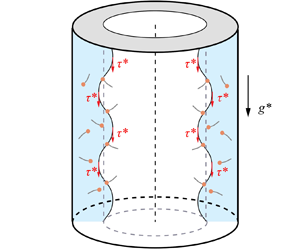
Jain, Neha
and
Sharma, Gaurav
2025.
Effect of imposed shear stress on the stability of surfactant-laden liquid film flow over a rod.
European Journal of Mechanics - B/Fluids,
Vol. 111,
Issue. ,
p.
229.