Adversarial consistency and the uniqueness of the adversarial bayes classifier

Abstract

Minimizing an adversarial surrogate risk is a common technique for learning robust classifiers. Prior work showed that convex surrogate losses are not statistically consistent in the adversarial context – or in other words, a minimizing sequence of the adversarial surrogate risk will not necessarily minimize the adversarial classification error. We connect the consistency of adversarial surrogate losses to properties of minimizers to the adversarial classification risk, known as adversarial Bayes classifiers. Specifically, under reasonable distributional assumptions, a convex surrogate loss is statistically consistent for adversarial learning iff the adversarial Bayes classifier satisfies a certain notion of uniqueness.

1. Introduction

Robustness is a core concern in machine learning, as models are deployed in classification tasks such as facial recognition [36], medical imaging [25] and identifying traffic signs in self-driving cars [13]. Deep learning models exhibit a concerning security risk – small perturbations imperceptible to the human eye can cause a neural net to misclassify an image [9, 32]. The machine learning literature has proposed many defenses, but many of these techniques remain poorly understood. This paper analyzes the statistical consistency of a popular defense method that involves minimizing an adversarial surrogate risk.

The central goal in a classification task is minimizing the proportion of mislabeled data-points – also known as the classification risk. Minimizers to the classification risk are easy to compute analytically and are known as Bayes classifiers. In the adversarial setting, each point is perturbed by a malicious adversary before the classifier makes a prediciton. The proportion of mislabelled data under such an attack is called the adversarial classification risk, and minimizers to this risk are called adversarial Bayes classifiers. Unlike the standard classification setting, computing minimizers to the adversarial classification risk is a nontrivial task [8, 27]. Further studies [15, 18, 28, 33, 35] investigate additional properties of these minimizers, and Frank [15] describes a notion of uniqueness for adversarial Bayes classifiers. The main result in this paper will connect this notion of uniqueness the statistical consistency of a popular defense method.

The empirical adversarial classification error is a discrete notion and minimizing this quantity is computationally intractable. Instead, typical machine learning algorithms minimize a surrogate risk in place of the classification error. In the robust setting, the adversarial training algorithm uses a surrogate risk that computes the supremum of loss over the adversary’s possible attacks, which we refer to as adversarial surrogate risks. However, one must verify that minimizing this adversarial surrogate will also minimize the classification risk. A loss function is adversarially consistent for a particular data distribution if every minimizing sequence of the associated adversarial surrogate risk also minimizes the adversarial classification risk. A loss is simply called adversarially consistent if it is adversarially consistent for all possible data distributions. Surprisingly, Meunier et al. [23] show that no convex surrogate is adversarially consistent, in contrast to the standard classification setting where most convex losses are statistically consistent [6, 22, 24, 31, 37].

Our contributions. We relate the statistical consistency of losses in the adversarial setting to the uniqueness of the adversarial Bayes classifier. Specifically, under reasonable assumptions, a convex loss is adversarially consistent for a specific data distribution iff the adversarial Bayes classifier is unique.

Prior work [15] further demonstrates several distributions for which the adversarial Bayes classifier is unique, and thus a typical convex loss would be consistent. Understanding general conditions under which uniqueness occurs is an open question.

Paper outline. Section 2 discusses related works, and Section 3 presents the problem background. Section 4 states our main theorem and presents some examples. Subsequently, Section 5 discusses intermediate results necessary for proving our main theorem. Next, our consistency results are proved in Sections 6 and 7. Appendices A and B present deferred proofs from Section 5, while Appendix C presents deferred proofs on surrogate risks from Sections 5 and 6. Finally, Appendix D presents deferred proofs from Section 7.

2. Related works

Our results are inspired by prior work that showed that no convex loss is adversarially consistent [3, 23] yet a wide class of adversarial losses is adversarially consistent [16]. These consistency results rely on the theory of surrogate losses, studied by Bartlett et al. [6], Lin [22] in the standard classification setting; and by Frank and Niles-Weed Frank and Niles-Weed [17], Li and Telgarsky [21] in the adversarial setting. Furthermore, [2, 5, 31] study a property of related to consistency called calibration, which [23] relate to consistency. Complimenting this analysis, another line of research studies $\mathcal {H}$ -consistency, which refines the concept of consistency to specific function classes [3, 26]. Our proof combines results on losses with minimax theorems for various adversarial risks, as studied by [16, 17, 28, 34].

Furthermore, our result leverages recent results on the adversarial Bayes classifier, which are extensively studied by [4, 8, 10, 16, 27, 28]. Specifically, [4, 8, 10] prove the existence of the adversarial Bayes classifier, while Trillos and Murray [33] derive necessary conditions that describe the boundary of the adversarial Bayes classifier. Frank [15] defines the notion of uniqueness up to degeneracy and proves that in one dimension, under reasonable distributional assumptions, every adversarial Bayes classifier is equivalent up to degeneracy to an adversarial Bayes classifier which satisfies the necessary conditions of [33]. Finally, [8, 27] also calculate the adversarial Bayes classifier for distributions in dimensions higher than one by finding an optimal coupling, but whether this method can calculate the equivalence classes under equivalence up to degeneracy remains an open question.

3. Notation and background

3.1 Surrogate risks

This paper investigates binary classification on $\mathbb {R}^d$ with labels $\{-1,+1\}$ . Class $-1$ is distributed according to a measure ${\mathbb P}_0$ while class $+1$ is distributed according to measure ${\mathbb P}_1$ . A classifier is a Borel set $A$ and the classification risk of a set $A$ is the expected proportion of errors when label $+1$ is predicted on $A$ and label $-1$ is predicted on $A^C$ :

\begin{align*} R(A)=\int {\mathbf {1}}_{A^C} d{\mathbb P}_1+\int {\mathbf {1}}_{A}d{\mathbb P}_0. \end{align*}

A minimizer to $R$ is called a Bayes classifier.

However, minimizing the empirical classification risk is a computationally intractable problem [7]. A common approach is to instead learn a function $f$ and then threshold at zero to obtain the classifier $A=\{{\mathbf x}\,:\, f({\mathbf x})\gt 0\}$ . We define the classification risk of a function $f$ by

(1) \begin{align} R(f)=R(\{f\gt 0\})=\int {\mathbf {1}}_{f\leq 0}d{\mathbb P}_1+\int {\mathbf {1}}_{{-}f\lt 0}d{\mathbb P}_0 \end{align}

Figure 1. Several common loss functions for classification along with the indicator ${\mathbf {1}}_{\alpha \leq 0}$ .

In order to learn $f$ , machine learning algorithms typically minimize a better-behaved alternative to the classification risk called a surrogate risk. To obtain this risk, we replace the indicator functions in (1) with the loss $\phi$ , resulting in:

(2) \begin{align} R_\phi (f)=\int \phi (f)d{\mathbb P}_1+\int \phi ({-}f) d{\mathbb P}_0\,. \end{align}

We restrict to losses with similar properties to the indicator functions in (1) yet are easier to optimize. In particular we require:

Assumption 1. The loss $\phi$ is nonincreasing, continuous, and $\lim _{\alpha \to \infty } \phi (\alpha )=0$ .

See Figure 1 for a comparison of the indicator function and a several common losses. Losses on $\mathbb {R}$ -valued functions in machine learning typically satisfy Assumption1.

3.2 Adversarial surrogate risks

In the adversarial setting, a malicious adversary corrupts each data point. We model these corruptions as bounded by $\epsilon$ in some norm $\|\cdot \|$ . The adversary knows both the classifier $A$ and the label of each data point. Thus, a point $({\mathbf x},+1)$ is misclassified when it can be displaced into the set $A^C$ by a perturbation of size at most $\epsilon$ . This statement can be conveniently written in terms of a supremum. For any function $g\,:\,\mathbb {R}^d\to \mathbb {R}$ , define

\begin{align*} S_\epsilon (g)({\mathbf x})=\sup _{{\mathbf x}^{\prime} \in \overline {B_\epsilon ({\mathbf x})}} g({\mathbf x}^{\prime}), \end{align*}

where $\overline {B_\epsilon ({\mathbf x})}=\{{\mathbf x}^{\prime}\,:\,\|{\mathbf x}^{\prime}-{\mathbf x}\|\leq \epsilon \}$ is the ball of allowed perturbations. The expected error rate of a classifier $A$ under an adversarial attack is then

\begin{align*} R^\epsilon (A)=\int S_\epsilon ({\mathbf {1}}_{A^C}) d{\mathbb P}_1+\int S_\epsilon ({\mathbf {1}}_{A})d{\mathbb P}_0, \end{align*}

which is known as the adversarial classification risk.¹ Minimizers of $R^\epsilon$ are called adversarial Bayes classifiers.

Just like (1), we define $R^\epsilon (f)=R^\epsilon (\{f\gt 0\})$ :

\begin{align*} R^\epsilon (f)=\int S_\epsilon ({\mathbf {1}}_{f\leq 0})d{\mathbb P}_1+\int S_\epsilon ({\mathbf {1}}_{f\gt 0})d{\mathbb P}_0 \end{align*}

Again, minimizing an empirical adversarial classification risk is computationally intractable. A surrogate to the adversarial classification risk is formulated as ²

(3) \begin{align} R_\phi ^\epsilon (f)=\int S_\epsilon ( \phi \circ f)d{\mathbb P}_1 +\int S_\epsilon ( \phi \circ -f)d{\mathbb P}_0. \end{align}

3.3 The statistical consistency of surrogate risks

Learning algorithms typically minimize a surrogate risk using an iterative procedure, thereby producing a sequence of functions $f_n$ . One would hope that that $f_n$ also minimizes that corresponding classification risk. This property is referred to as statistical consistency. ³

Definition 1.

• • If every sequence of functions $f_n$ that minimizes $R_\phi$ also minimizes $R$ for the distribution ${\mathbb P}_0,{\mathbb P}_1$ , then the loss $\phi$ is consistent for the distribution ${\mathbb P}_0,{\mathbb P}_1$ . If $R_\phi$ is consistent for every distribution ${\mathbb P}_0,{\mathbb P}_1$ , we say that $\phi$ is consistent.

• • If every sequence of functions $f_n$ that minimizes $R_\phi ^\epsilon$ also minimizes $R^\epsilon$ for the distribution ${\mathbb P}_0,{\mathbb P}_1$ , then the loss $\phi$ is adversarially consistent for the distribution ${\mathbb P}_0,{\mathbb P}_1$ . If $R_\phi ^\epsilon$ is adversarially consistent for every distribution ${\mathbb P}_0,{\mathbb P}_1$ , we say that $\phi$ is adversarially consistent.

A case of particular interest is convex $\phi$ , as these losses are ubiquitous in machine learning. In the non-adversarial context, Theorem2 of [6] shows that a convex loss $\phi$ is consistent iff $\phi$ is differentiable at zero and $\phi ^{\prime}(0)\lt 0$ . In contrast, Meunier et al. [23] show that no convex loss is adversarially consistent. Further results of [16] characterize the adversarially consistent losses in terms of the function $C_\phi ^*$ :

Theorem 1. The loss $\phi$ is adversarially consistent if and only if $C_\phi ^*(1/2)\lt \phi (0)$ .

Notice that all convex losses satisfy $C_\phi ^*(1/2)=\phi (0)$ : By evaluating at $\alpha =0$ , one can conclude that $C_\phi ^*(1/2)= \inf _\alpha C_\phi (1/2,\alpha )\leq C_\phi (1/2,0)=\phi (0)$ . However,

\begin{align*} C_\phi ^*(1/2)=\inf _\alpha \frac 12 \phi (\alpha )+\frac 12 \phi (-\alpha )\geq \phi (0) \end{align*}

due to convexity. Notice that Theorem1 does not preclude the adversarial consistency of a loss satisfying $C_\phi ^*(1/2)=\phi (0)$ for some particular ${\mathbb P}_0,{\mathbb P}_1$ . Prior work [16, 23] provides a counterexample to consistency only for a single, atypical distribution. The goal of this paper is characterizing when adversarial consistency fails for losses satisfying $C_\phi ^*(1/2)=\phi (0)$ .

4. Main result

Prior work has shown that there always exists minimizers to the adversarial classification risk, which are referred to as adversarial Bayes classifiers (see Theorem3 below). Furthermore, Frank [15] developed a notion of uniqueness for adversarial Bayes classifiers.

Definition 2. The adversarial Bayes classifiers $A_1$ and $A_2$ are equivalent up to degeneracy if any Borel set $A$ with $A_1\cap A_2\subset A\subset A_1\cup A_2$ is also an adversarial Bayes classifier. The adversarial Bayes classifier is unique up to degeneracy if any two adversarial Bayes classifiers are equivalent up to degeneracy.

When the measure

\begin{align*} {\mathbb P}={\mathbb P}_0+{\mathbb P}_1 \end{align*}

is absolutely continuous with respect to Lebesgue measure, then equivalence up to degeneracy is an equivalence relation [15, Theorem 3.3]. The central result of this paper relates the consistency of convex losses to the uniqueness of the adversarial Bayes classifier.

Theorem 2. Assume that $\mathbb P$ is absolutely continuous with respect to Lebesgue measure and let $\phi$ be a loss with $C_\phi ^*(1/2)=\phi (0)$ . Then $\phi$ is adversarially consistent for the distribution ${\mathbb P}_0$ , ${\mathbb P}_1$ iff the adversarial Bayes classifier is unique up to degeneracy.

Prior results of Frank [15] provide the tools for verifying when the adversarial Bayes classifier is unique up to degeneracy for a wide class of one dimensional distributions. Below we highlight two interesting examples. In the examples below, the function $p_1$ will represent the density of ${\mathbb P}_1$ and the function $p_0$ will represent the density of ${\mathbb P}_0$ .

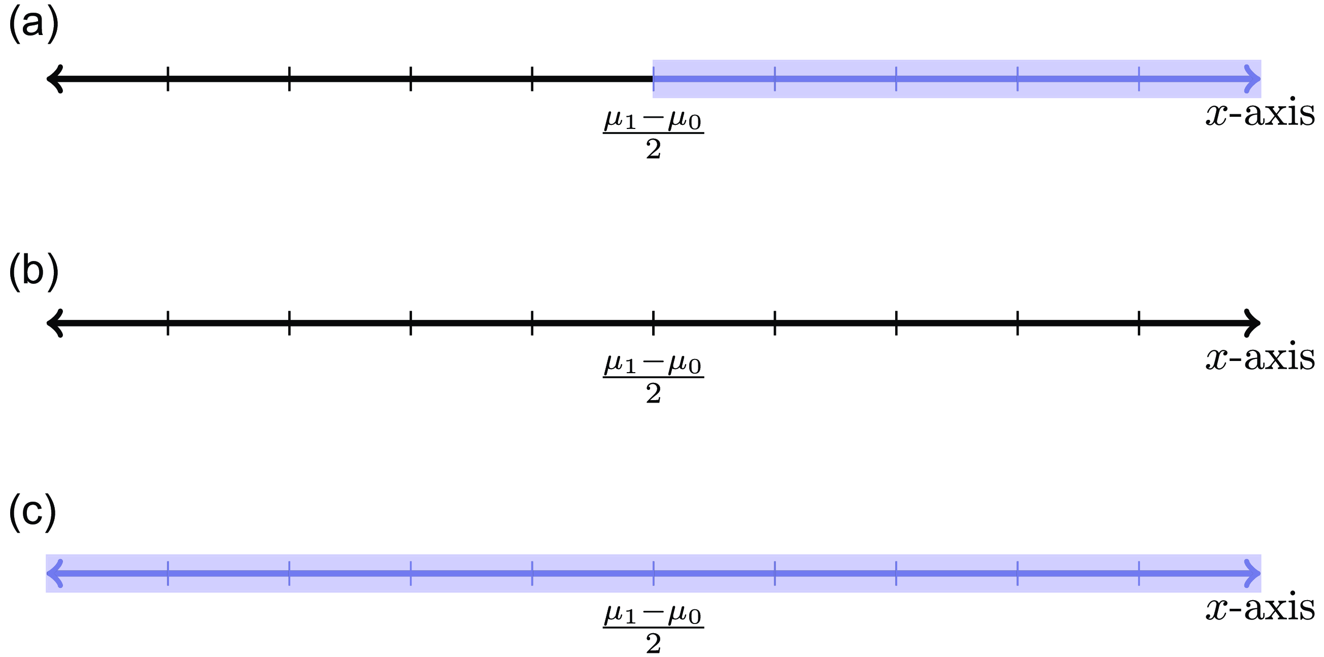
Figure 2. The adversarial Bayes classifier for two gaussians with equal variances and differing means. We assume in this figure that $\mu _1\gt \mu _0$ . The shaded blue area depicts the region inside the adversarial Bayes classifier. Figure 2a depicts an adversarial Bayes when $\epsilon \leq (\mu _1-\mu _0)/2$ and Figure 2b and 2c depict the adversarial Bayes classifier when $\epsilon \geq (\mu _1-\mu _0)/2$ . (See [15, Example 4.1] for a justification of these illustrations.) the adversarial Bayes classifiers in Figure 2b and 2c are not equivalent up to degeneracy.

• • Consider mean zero gaussians with different variances: $p_0(x)=\frac 1 {2\sqrt {2\pi } \sigma _0}e^{-x^2/2\sigma _0^2}$ and $p_1(x)=\frac 1 {2\sqrt {2\pi } \sigma _1}e^{-x^2/2\sigma _1^2}$ . The adversarial Bayes classifier is unique up to degeneracy for all $\epsilon$ [15, Example 4.2].

• • Consider gaussians with variance $\sigma$ and means $\mu _0$ and $\mu _1$ : $p_0(x)=\frac 1 {\sqrt {2\pi } \sigma }e^{-(x-\mu _0)^2/2\sigma ^2}$ and $p_1(x)=\frac 1 {\sqrt {2\pi } \sigma }e^{-(x-\mu _1)^2/2\sigma ^2}$ . Then the adversarial Bayes classifier is unique up to degeneracy iff $\epsilon \lt |\mu _1-\mu _0|/2$ [15, Example 4.1]. See Figure 2 for an illustration of the adversarial Bayes classifiers for this distribution.

Theorem2 implies that a convex loss is always adversarially consistent for the first gaussian mixture above. Furthermore, a convex loss is adversarially consistent for the second gaussian mixture when the perturbation radius $\epsilon$ is small compared to the differences between the means. However, Frank [15, Example 4.5] provides an example of a distribution for which the adversarial Bayes classifier is not unique up to degeneracy for all $\epsilon \gt 0$ , even though the Bayes classifier is unique. At the same time, one would hope that if the Bayes classifier is unique and ${\mathbb P}_0$ , ${\mathbb P}_1$ are sufficiently regular, then the adversarial Bayes classifier would be unique up to degeneracy for sufficiently small $\epsilon$ . In general, understanding when the adversarial Bayes classifier is unique up to degeneracy for well-behaved distributions is an open problem.

The examples above rely on the techniques of [15] for calculating the equivalence classes under uniqueness up to degeneracy. Frank [15] proves that in one dimension, if $\mathbb P$ is absolutely continuous with respect to Lebesgue measure, every adversarial Bayes classifier is equivalent up to degeneracy to an adversarial Bayes classifier whose boundary points are strictly more than $2\epsilon$ apart [15, Theorem 3.5]. Therefore, to find all adversarial Bayes classifiers under equivalence under degeneracy, it suffices to consider all sets whose boundary points satisfy the first order necessary conditions obtained by differentiating the adversarial classification risk of a set $A$ with respect to its boundary points [15, Theorem 3.7]. The corresponding statement in higher dimensions is false – there exist distributions for which no adversarial Bayes classifier has enough regularity to allow for an equivalent statement. For instance, Bungert et al. [10] demonstrate a distribution for which there is no adversarial Bayes classifier with two-sided tangent balls at all points in the boundary. Developing a general method for calculating these equivalence classes in dimensions higher than one remains an open problem.

Proposition2 in Section 6 presents a condition under which one can conclude consistency without the absolute continuity assumption. This result proves consistency whenever the optimal adversarial classification risk is zero, see the discussion after Proposition2 for details. Consequently, if $\mathrm {supp} {\mathbb P}_0$ and $\mathrm {supp} {\mathbb P}_1$ are separated by more than $2\epsilon$ , then consistent losses are always adversarially consistent for such distributions. On the other hand, our analysis of the reverse direction of Theorem2 requires the absolute continuity assumption. Using Proposition2 to further understand consistency is an open question.

5. Preliminary results

5.1 Minimizers of standard risks

Minimizers to the classification risk can be expressed in terms of the measure $\mathbb P$ and the function $\eta =d{\mathbb P}_1/d{\mathbb P}$ . The risk $R$ in terms of these quantities is

\begin{align*} R(A)= \int C(\eta, {\mathbf {1}}_A)d{\mathbb P}. \end{align*}

and $\inf _A R(A)=\int C^*(\eta )d{\mathbb P}$ where the functions $C\,:\,[0,1]\times \{0,1\}\to \mathbb {R}$ and $C^*\,:\,[0,1]\to \mathbb {R}$ are defined by

(4) \begin{align} C(\eta, b)=\eta b+(1-\eta )(1-b),\quad C^*(\eta )=\inf _{b\in \{0,1\}} C(\eta, b)=\min \!(\eta, 1-\eta ). \end{align}

Thus, if $A$ is a minimizer of $R$ , then ${\mathbf {1}}_A$ must minimize the function $C(\eta, \cdot )$ $\mathbb P$ -almost everywhere. Consequently, the sets

(5) \begin{align} \{{\mathbf x}\,:\,\eta ({\mathbf x})\gt 1/2\} \quad \text {and} \quad \{{\mathbf x}\,:\,\eta ({\mathbf x})\geq 1/2\} \end{align}

are both Bayes classifiers.

Similarly, one can compute the infimum of $R_\phi$ by expressing the risk in terms of the quantities $\mathbb P$ and $\eta$ :

(6) \begin{align} R_\phi (f)=\int C_\phi (\eta ({\mathbf x}),f({\mathbf x}))d{\mathbb P} \end{align}

and $\inf _f R_\phi (f)=\int C_\phi ^*(\eta ({\mathbf x}))d{\mathbb P}({\mathbf x})$ where the functions $C_\phi (\eta, \alpha )$ and $C_\phi ^*(\eta )$ are defined by

(7) \begin{align} C_\phi (\eta, \alpha ) = \eta \phi (\alpha )+(1-\eta )\phi (-\alpha ),\quad C_\phi ^*(\eta )=\inf _\alpha C_\phi (\eta, \alpha ) \end{align}

for $\eta \in [0,1]$ . Thus, a minimizer $f$ of $R_\phi$ must minimize $C_\phi (\eta ({\mathbf x}),\cdot )$ almost everywhere according to the probability measure $\mathbb P$ . Because $\phi$ is continuous, the function

(8) \begin{align} \alpha _\phi (\eta )=\inf \{\alpha \in \overline {\mathbb {R}}\,:\, \alpha \text { is a minimizer of }C_\phi (\eta, \cdot )\} \end{align}

maps each $\eta$ to the smallest minimizer of $C_\phi (\eta, \cdot )$ . Consequently, the function

(9) \begin{align} \alpha _\phi (\eta ({\mathbf x})) \end{align}

minimizes $C_\phi (\eta ({\mathbf x}),\cdot )$ at each point $\mathbf x$ . Next, we will argue this function is measurable, and therefore is a minimizer of the risk $R_\phi$ .

Lemma 1. The function $\alpha _\phi \,:\,[0,1]\to \overline {\mathbb {R}}$ that maps $\eta$ to the smallest minimizer of $C_\phi (\eta, \cdot )$ is non-decreasing.

The proof of this result is presented below Lemma7 in Appendix C. Because $\alpha _\phi$ is monotonic, the composition in (9) is always measurable, and thus this function is a minimizer of $R_\phi$ . Allowing for minimizers in extended real numbers $\overline {\mathbb {R}}=\{-\infty, +\infty \}\cup \mathbb {R}$ is necessary for certain losses – for instance when $\phi$ is the exponential loss, then $C_\phi (1,\alpha )= e^{-\alpha }$ does not assume its infimum on $\mathbb {R}$ .

5.2 Dual problems for the adversarial risks

The proof Theorem2 relies on a dual formulation of the adversarial classification problem involving the Wasserstein- $\infty$ metric. Informally, a measure ${\mathbb Q}^{\prime}$ is within $\epsilon$ of $\mathbb Q$ in the Wasserstein- $\infty$ metric if one can produce ${\mathbb Q}^{\prime}$ by perturbing each point in $\mathbb {R}^d$ by at most $\epsilon$ under the measure $\mathbb Q$ . The formal definition of the Wasserstein- $\infty$ metric involves couplings between probability measures: a coupling between two Borel measures $\mathbb Q$ and ${\mathbb Q}^{\prime}$ with ${\mathbb Q}(\mathbb {R}^d)={\mathbb Q}^{\prime}(\mathbb {R}^d)$ is a measure $\gamma$ on $\mathbb {R}^d\times \mathbb {R}^d$ with marginals $\mathbb Q$ and ${\mathbb Q}^{\prime}$ : $\gamma (A\times \mathbb {R}^d)={\mathbb Q}(A)$ and $\gamma (\mathbb {R}^d\times A)={\mathbb Q}^{\prime}(A)$ for any Borel set $A$ . The set of all such couplings is denoted $\Pi ({\mathbb Q},{\mathbb Q}^{\prime})$ . The Wasserstein- $\infty$ distance between the two measures is then

\begin{align*} W_\infty ({\mathbb Q},{\mathbb Q}^{\prime})= \inf _{\gamma \in \Pi ({\mathbb Q},{\mathbb Q}^{\prime})} \mathop {\textrm{ess sup}}\limits_{({\mathbf x},{\mathbf x}^{\prime})\sim \gamma } \|{\mathbf x}-{\mathbf x}^{\prime}\| \end{align*}

Theorem 2.6 of [19] proves that this infimum is always assumed. Equivalently, $W_\infty ({\mathbb Q},{\mathbb Q}^{\prime})\leq \epsilon$ iff there is a coupling between $\mathbb Q$ and ${\mathbb Q}^{\prime}$ supported on

\begin{align*} \Delta _\epsilon =\{({\mathbf x},{\mathbf x}^{\prime})\,:\, \|{\mathbf x}-{\mathbf x}^{\prime} \|\leq \epsilon \}. \end{align*}

Let ${{\mathcal {B}}^\infty _{\epsilon }}({\mathbb Q})=\{{\mathbb Q}^{\prime}\,:\, W_\infty ({\mathbb Q},{\mathbb Q}^{\prime})\leq \epsilon \}$ be the set of measures within $\epsilon$ of $\mathbb Q$ in the $W_\infty$ metric. The minimax relations from prior work leverage a relationship between the Wasserstein- $\infty$ metric and the integral of the supremum function over an $\epsilon$ -ball.

Lemma 2. Let $E$ be a Borel set. Then

\begin{align*} \int S_\epsilon ({\mathbf {1}}_E)d{\mathbb Q}\geq \sup _{{\mathbb Q}^{\prime}\in {{\mathcal {B}}^\infty _{\epsilon }}({\mathbb Q}) } \int {\mathbf {1}}_E d{\mathbb Q}^{\prime} \end{align*}

Proof. Let ${\mathbb Q}^{\prime}$ be a measure in ${{\mathcal {B}}^\infty _{\epsilon }} ({\mathbb Q})$ , and let $\gamma ^*$ be a coupling between these two measures supported on $\Delta _\epsilon$ . Then if $({\mathbf x},{\mathbf x}^{\prime})\in \Delta _\epsilon$ , then ${\mathbf x}^{\prime}\in \overline {B_\epsilon ({\mathbf x})}$ and thus $S_\epsilon ({\mathbf {1}}_E)({\mathbf x})\geq {\mathbf {1}}_E({\mathbf x}^{\prime})$ $\gamma ^*$ -a.e. Consequently,

\begin{align*} \int S_\epsilon ({\mathbf {1}}_E)({\mathbf x})d{\mathbb Q}_1=\int S_\epsilon ({\mathbf {1}}_E)({\mathbf x})d\gamma ^*({\mathbf x},{\mathbf x}^{\prime})\geq \int {\mathbf {1}}_E({\mathbf x}^{\prime}) d\gamma ^*({\mathbf x},{\mathbf x}^{\prime})=\int {\mathbf {1}}_E d{\mathbb Q}^{\prime} \end{align*}

Taking a supremum over all ${\mathbb Q}^{\prime}\in {{\mathcal {B}}^\infty _{\epsilon }}({\mathbb Q})$ proves the result.

Lemma2 implies:

\begin{align*} \inf _f R^\epsilon (f)\geq \inf _f\sup _{\substack {{\mathbb P}_1^{\prime}\in {\mathcal {B}}_\epsilon ({\mathbb P}_1)\\ {\mathbb P}_0^{\prime}\in {\mathcal {B}}_\epsilon ({\mathbb P}_0) }}\int {\mathbf {1}}_{f\leq 0} d{\mathbb P}_1^{\prime}+\int {\mathbf {1}}_{f\gt 0} d{\mathbb P}_0^{\prime}. \end{align*}

Does equality hold and can one swap the infimum and the supremum? Frank and Niles-Weed [16], Pydi and Jog [28] answer this question in the affirmative:

Theorem 3. Let ${\mathbb P}_0$ , ${\mathbb P}_1$ be finite Borel measures. Define

\begin{align*} \bar R({\mathbb P}_0^*,{\mathbb P}_1^*)=\int C^*\left (\frac {d{\mathbb P}_1^*}{d({\mathbb P}_0^*+d{\mathbb P}_1^*)} \right )d({\mathbb P}_0^*+{\mathbb P}_1^*) \end{align*}

where the function $C^*$ is defined in ( 4 ). Then

\begin{align*} \inf _{\substack {f\text { Borel}\\\mathbb {R}\text {-valued}}} R^\epsilon (f)=\sup _{\substack {{\mathbb P}_1^{\prime}\in {{\mathcal {B}}^\infty _{\epsilon }}({\mathbb P}_1)\\{\mathbb P}_0^{\prime}\in {{\mathcal {B}}^\infty _{\epsilon }}({\mathbb P}_0)}}\bar R({\mathbb P}_0^{\prime},{\mathbb P}_1^{\prime}) \end{align*}

and furthermore equality is attained for some $f^*$ , ${\mathbb P}_0^*$ , ${\mathbb P}_1^*$ .

See Theorem1 of [16] for a proof. Theorems6, 8, and 9 of [17] show an analogous minimax theorem for surrogate risks.

Theorem 4. Let ${\mathbb P}_0$ , ${\mathbb P}_1$ be finite Borel measures. Define

\begin{align*} {\bar {R}_\phi }({\mathbb P}_0^*,{\mathbb P}_1^*)=\int C_\phi ^*\left (\frac {d{\mathbb P}_1^*}{d({\mathbb P}_0^*+d{\mathbb P}_1^*)} \right )d({\mathbb P}_0^*+{\mathbb P}_1^*) \end{align*}

with the function $C_\phi ^*$ is defined in ( 7 ). Then

\begin{align*} \inf _{\substack {f\text { Borel,}\\\overline {\mathbb {R}}\text {-valued}}} R_\phi ^\epsilon (f)=\sup _{\substack {{\mathbb P}_0^{\prime}\in {{\mathcal {B}}^\infty _{\epsilon }}({\mathbb P}_0)\\ {\mathbb P}_1^{\prime}\in {{\mathcal {B}}^\infty _{\epsilon }}({\mathbb P}_1)}}{\bar {R}_\phi }({\mathbb P}_0^{\prime},{\mathbb P}_1^{\prime}) \end{align*}

and furthermore equality is attained for some $f^*$ , ${\mathbb P}_0^*$ , ${\mathbb P}_1^*$ .

Just like $R_\phi$ , the risk $R_\phi ^\epsilon$ may not have an $\mathbb {R}$ -valued minimizer. However, Lemma8 of [16] states that

\begin{align*} \inf _{\substack {f\text { Borel}\\\overline {\mathbb {R}}\text {-valued}}} R_\phi ^\epsilon (f)=\inf _{\substack {f\text { Borel}\\ \mathbb {R}\text {-valued}}} R_\phi ^\epsilon (f). \end{align*}

5.3 Minimizers of adversarial risks

A formula analogous to (9) defines minimizers to adversarial risks. Let $I_\epsilon$ denote the infimum of a function over an $\epsilon$ ball:

(10) \begin{align} I_\epsilon (g)=\inf _{{\mathbf x}^{\prime}\in \overline {B_\epsilon ({\mathbf x})}}g({\mathbf x}^{\prime}) \end{align}

Lemma 24 of [17] and Theorem9 of [17] prove the following result:

Theorem 5. There exists a function $\hat \eta \,:\, \mathbb {R}^d\to [0,1]$ and measures ${\mathbb P}_0^*\in {{\mathcal {B}}^\infty _{\epsilon }} ({\mathbb P}_0)$ , ${\mathbb P}_1^*\in {{\mathcal {B}}^\infty _{\epsilon }} ({\mathbb P}_1)$ for which

1. I) $\hat \eta =\eta ^*$ ${\mathbb P}^*$ -a.e., where ${\mathbb P}^*={\mathbb P}_0^*+{\mathbb P}_1^*$ and $\eta ^*=d{\mathbb P}_1^*/d{\mathbb P}^*$

2. II) $I_\epsilon (\hat \eta )({\mathbf x})=\hat \eta ({\mathbf x}^{\prime})$ $\gamma _0^*$ -a.e. and $S_\epsilon (\hat \eta )({\mathbf x})=\hat \eta ({\mathbf x}^{\prime})$ $\gamma _1^*$ -a.e., where $\gamma _0^*$ , $\gamma _1^*$ are couplings between ${\mathbb P}_0$ , ${\mathbb P}_0^*$ and ${\mathbb P}_1$ , ${\mathbb P}_1^*$ supported on $\Delta _\epsilon$ .

3. III) The function $\alpha _\phi (\hat \eta ({\mathbf x}))$ is a minimizer of $R_\phi ^\epsilon$ for any loss $\phi$ , where $\alpha _\phi$ is the function defined in ( 8 ).

The function $\hat \eta$ can be viewed as the conditional probability of label $+1$ under an ‘optimal’ adversarial attack [17]. Just as in the standard learning scenario, the function $\alpha (\hat \eta ({\mathbf x}))$ may be $\overline {\mathbb {R}}$ -valued. Item 3 is actually a consequence of Item 1 and Item 2: Item 1 and Item 2 imply that $R_\phi ^\epsilon (\alpha _\phi (\hat \eta ))={\bar {R}_\phi }({\mathbb P}_0^*,{\mathbb P}_1^*)$ and Theorem4 then implies that $\alpha _\phi (\hat \eta )$ minimizes $R_\phi ^\epsilon$ and ${\mathbb P}_0^*$ , ${\mathbb P}_1^*$ maximize $\bar {R}_\phi$ . (A similar argument is provided later in this paper in Lemma6 of Appendix D.1.) Furthermore, the relation $R_\phi ^\epsilon (\alpha _\phi (\hat \eta ))={\bar {R}_\phi }({\mathbb P}_0^*,{\mathbb P}_1^*)$ also implies

Lemma 3. The ${\mathbb P}_0^*$ , ${\mathbb P}_1^*$ of Theorem 5 maximize $\bar {R}_\phi$ over ${{\mathcal {B}}^\infty _{\epsilon }}({\mathbb P}_0)\times {{\mathcal {B}}^\infty _{\epsilon }}({\mathbb P}_1)$ for every $\phi$ .

We emphasize that a formal proof of Theorems5 and 3 is not included in this paper, and refer to Lemma 26 and Theorem9 of [17] for full arguments.

Next, we derive some further results about the function $\hat \eta$ . Recall that Bayes classifiers can be constructed by thesholding the conditional probability $\eta$ at $1/2$ , see Equation 5). The function $\hat \eta$ plays an analogous role for adversarial learning.

Theorem 6. Let $\hat \eta$ be the function described by Theorem 5 . Then the sets $\{\hat \eta \gt 1/2\}$ and $\{\hat \eta \geq 1/2\}$ are adversarial Bayes classifiers. Furthermore, any adversarial Bayes classifier $A$ satisfies

(11) \begin{align} \int S_\epsilon ({\mathbf {1}}_{\{\hat \eta \geq 1/2\}^C})d{\mathbb P}_1\leq \int S_\epsilon ({\mathbf {1}}_{A^C})d{\mathbb P}_1\leq \int S_\epsilon ({\mathbf {1}}_{\{\hat \eta \gt 1/2)^C})d{\mathbb P}_1 \end{align}

and

(12) \begin{align} \int S_\epsilon ({\mathbf {1}}_{\{\hat \eta \gt 1/2\}})d{\mathbb P}_0\leq \int S_\epsilon ({\mathbf {1}}_{A})d{\mathbb P}_0\leq \int S_\epsilon ({\mathbf {1}}_{\{\hat \eta \geq 1/2\}})d{\mathbb P}_0 \end{align}

See Appendix A for a formal proof; these properties follow direction from Item 1 and Item 2 of Theorem5. Equations (11) and (12) imply that the sets $\{\hat \eta \gt 1/2\}$ and $\{\hat \eta \geq 1/2\}$ can be viewed as ‘minimal’ and ‘maximal’ adversarial Bayes classifiers.

Theorem6 is proved in Appendix A– Item 1 and Item 2 imply that $ R^\epsilon (\{\hat \eta \gt 1/2\})=\bar R({\mathbb P}_0^*,{\mathbb P}_1^*)=R^\epsilon (\hat \eta \geq 1/2\})$ and consequently Theorem3 implies that $\{\hat \eta \gt 1/2\}$ , $\{\hat \eta \geq 1/2\}$ minimize $R^\epsilon$ and ${\mathbb P}_0^*$ , ${\mathbb P}_1^*$ maximize $\bar R$ . This proof technique is analogous to the approach employed by [17] to establish Theorem5. Lastly, uniqueness up to degeneracy can be characterized in terms of these ${\mathbb P}_0^*$ , ${\mathbb P}_1^*$ .

Theorem 7. Assume that $\mathbb P$ is absolutely continuous with respect to Lebesgue measure. Then the following are equivalent:

1. A) The adversarial Bayes classifier is unique up to degeneracy

2. B) ${\mathbb P}^*(\eta ^*=1/2)=0$ , where ${\mathbb P}^*={\mathbb P}_0^*+{\mathbb P}_1^*$ and $\eta ^*=d{\mathbb P}_1^*/d{\mathbb P}^*$ for the measures ${\mathbb P}_0^*,{\mathbb P}_1^*$ of Theorem 5 .

See Appendix B for a proof of Theorem7. In relation to prior work – the proof of [15, Theorem 3.4] shows Theorem7 but a full proof of Theorem7 is included in this paper for clarity as [15] did not discuss the role of the function $\hat \eta$ .

6. Uniqueness up to degeneracy implies consistency

Before presenting the full proof of consistency, we provide an overview of the strategy of this argument. First, a minimizing sequence of $R_\phi ^\epsilon$ must satisfy the approximate complementary slackness conditions derived in [16, Proposition 4].

Proposition 1. Assume that the measures ${\mathbb P}_0^*\in {{\mathcal {B}}^\infty _{\epsilon }}({\mathbb P}_0)$ , ${\mathbb P}_1^*\in {{\mathcal {B}}^\infty _{\epsilon }}({\mathbb P}_1)$ maximize $\bar {R}_\phi$ . Then any minimizing sequence $f_n$ of $R_\phi ^\epsilon$ must satisfyr

(13) \begin{align} \lim _{n\to \infty } \int C_\phi (\eta ^*,f_n)d{\mathbb P}^*= \int C_\phi ^*(\eta ^*)d{\mathbb P}^* \\[-18pt] \nonumber \end{align}

(14) \begin{align} \lim _{n\to \infty } \int S_\epsilon (\phi \circ f_n)d{\mathbb P}_1-\int \phi \circ f_nd{\mathbb P}_1^*=0, \quad \lim _{n\to \infty } \int S_\epsilon (\phi \circ -f_n) d{\mathbb P}_0- \int \phi \circ -f_nd{\mathbb P}_0^*=0, \\[6pt] \nonumber \end{align}

where ${\mathbb P}^*={\mathbb P}_0^*+{\mathbb P}_1^*$ and $\eta ^*=d{\mathbb P}_1^*/d{\mathbb P}^*$ .

We will show that when ${\mathbb P}^*(\eta ^*=1/2)=0$ , every sequence of functions satisfying (13) and (14) must minimize $R^\epsilon$ . Specifically, we will prove that every minimizing sequence $f_n$ of $R_\phi ^\epsilon$ must satisfy

(15) \begin{align} \limsup _{n\to \infty } \int S_\epsilon ({\mathbf {1}}_{f_n\leq 0}) d{\mathbb P}_1\leq \int {\mathbf {1}}_{\eta ^*\leq \frac 12} d{\mathbb P}_1^*, \\[-18pt] \nonumber \end{align}

(16) \begin{align} \limsup _{n\to \infty } \int S_\epsilon ({\mathbf {1}}_{f_n\geq 0}) d{\mathbb P}_0\leq \int {\mathbf {1}}_{\eta ^*\geq \frac 12} d{\mathbb P}_0^* \\[6pt] \nonumber \end{align}

for the measures ${\mathbb P}_0^*$ , ${\mathbb P}_1^*$ in Theorem5. Consequently, ${\mathbb P}^*(\eta ^*=1/2)=0$ would imply that $\limsup _{n\to \infty } R^\epsilon (f_n)\leq \bar R({\mathbb P}_0^*,{\mathbb P}_1^*)$ and the strong duality relation in Theorem3 implies that $f_n$ must in fact be a minimizing sequence of $R^\epsilon$ .

Next, we summarize the argument establishing Equation 15. We make several simplifying assumptions in the following discussion. First, we assume that the functions $\phi$ , $\alpha _\phi$ are strictly monotonic and that for each $\eta$ , there is a unique value of $\alpha$ for which $\eta \phi (\alpha )+(1-\eta )\phi (-\alpha )=C_\phi ^*(\eta )$ . (For instance, the exponential loss $\phi (\alpha )=e^{-\alpha }$ satisfies these requirements.) Let $\gamma _1^*$ be a coupling between ${\mathbb P}_1$ and ${\mathbb P}_1^*$ supported on $\Delta _\epsilon$ .

Because $C_\phi (\eta ^*,f_n)\geq C_\phi ^*(\eta ^*)$ , the condition (13) implies that $C_\phi (\eta ^*,f_n)$ converges to $C_\phi ^*(\eta ^*)$ in $L^1({\mathbb P}^*)$ , and the assumption that there is a single value of $\alpha$ for which $\eta \phi (\alpha )+(1-\eta )\phi (-\alpha )=C_\phi ^*(\eta )$ implies that the function $\phi (f_n({\mathbf x}^{\prime}))$ must converge to $\phi (\alpha _\phi (\eta ^*({\mathbf x}^{\prime}))$ in $L^1({\mathbb P}_1^*)$ . Similarly, because Lemma2 states that $S_\epsilon (\phi \circ f_n)({\mathbf x})\geq \phi \circ f_n({\mathbf x}^{\prime})$ $\gamma _1^*$ -a.e., Equation 14) implies that $S_\epsilon (\phi \circ f_n)({\mathbf x})-\phi \circ f_n({\mathbf x}^{\prime})$ converges to 0 in $L^1(\gamma _1^*)$ . Consequently $S_\epsilon (\phi \circ f_n)({\mathbf x})$ must converge to $\phi (\alpha _\phi (\eta ^*({\mathbf x}^{\prime})))$ in $L^1(\gamma _1^*)$ . As $L^1$ convergence implies convergence in measure [14, Proposition 2.29], one can conclude that

(17) \begin{align} \lim _{n\to \infty } \gamma _1^*\big (S_\epsilon (\phi \circ f_n)({\mathbf x})-\phi \circ ( \alpha _\phi (\hat \eta ({\mathbf x}^{\prime})))\gt c\big )=0 \end{align}

for any $c\gt 0$ . The lower semi-continuity of $\alpha \mapsto {\mathbf {1}}_{\alpha \leq 0}$ implies that $\int S_\epsilon ({\mathbf {1}}_{f_n\leq 0})d{\mathbb P}_1\leq \int {\mathbf {1}}_{S_\epsilon (\phi (f_n))({\mathbf x})\geq \phi (0)}d{\mathbb P}_1$ and furthermore (17) implies

(18) \begin{align} \limsup _{n\to \infty } \int {\mathbf {1}}_{S_\epsilon (\phi (f_n))({\mathbf x})\geq \phi (0)}d\gamma _1^*\leq \int {\mathbf {1}}_{\phi (\alpha _\phi (\eta ^*({\mathbf x}^{\prime})))\lt \phi (0)-c}d\gamma _1^* = \int {\mathbf {1}}_{\eta ^*\geq \alpha _\phi ^{-1}\circ \phi ^{-1}(\phi (0)-c)}d{\mathbb P}_1^*. \end{align}

Next, we will also assume that $\alpha _\phi ^{-1}$ is continuous and $\alpha _\phi (1/2)=0$ . (The exponential loss satisfies these requirements as well.) Due to our assumptions on $\phi$ and $\alpha _\phi$ , the quantity $\phi ^{-1}(\phi (0)-c)$ is strictly smaller than 0, and consequently, $\alpha _\phi ^{-1}\circ \phi ^{-1}(\phi (0)-c)$ is strictly smalaler than $1/2$ . However, if $\alpha _\phi ^{-1}$ is continuous, one can choose $c$ small enough so that ${\mathbb P}^*( |\eta -1/2|\lt 1/2- \alpha _\phi ^{-1}\circ \phi ^{-1}(\phi (0)-c))\lt \delta$ for any $\delta \gt 0$ when ${\mathbb P}^*(\eta ^*=1/2)=0$ . This choice of $c$ along with (18) proves (15).

To avoid the prior assumptions on $\phi$ and $\alpha$ , we prove that when $\eta$ is bounded away from $1/2$ and $\alpha$ is bounded away from the minimizers of $C_\phi (\eta, \cdot )$ , then $C_\phi (\eta, \alpha )$ is bounded away from $C_\phi ^*(\eta )$ .

Lemma 4. Let $\phi$ be a consistent loss. For all $r\gt 0$ , there is a constant $k_r\gt 0$ and an $\alpha _r\gt 0$ for which if $|\eta -1/2|\geq r$ and $\textrm {sign}(\eta -1/2) \alpha \leq \alpha _r$ then $C_\phi (\eta, \alpha _r)-C_\phi ^*(\eta )\geq k_r$ , and this $\alpha _r$ satisfies $\phi (\alpha _r)\lt \phi (0)$ .

See Appendix C for a proof. A minor modification of the argument above our main result:

Proposition 2. Assume there exist ${\mathbb P}_0^*\in {{\mathcal {B}}^\infty _{\epsilon }} ({\mathbb P}_0)$ , ${\mathbb P}_1^*\in {{\mathcal {B}}^\infty _{\epsilon }}({\mathbb P}_1)$ that maximize $\bar {R}_\phi$ for which ${\mathbb P}^*(\eta ^*=1/2)=0$ . Then any consistent loss is adversarially consistent.

When $\mathbb P$ is absolutely continuous with respect to Lebesgue measure, uniqueness up to degeneracy of the adversarial Bayes classifier implies the assumptions of this proposition due to Theorem7. However, this result applies even to distributions which are not absolutely continuous with respect to Lebesgue measure. For instance, if the optimal classification risk is zero, the ${\mathbb P}^*(\eta ^*=1/2)=0$ . To show this statement, notice that if $\inf _A R^\epsilon (A)=0$ , then Theorem3 implies that for any measures ${\mathbb P}_0^{\prime}\in {{\mathcal {B}}^\infty _{\epsilon }}({\mathbb P}_0)$ , ${\mathbb P}_1^{\prime}\in {{\mathcal {B}}^\infty _{\epsilon }}({\mathbb P}_1)$ , one can conclude that ${\mathbb P}^{\prime}(\eta ^{\prime}=1/2)=0$ , where ${\mathbb P}^{\prime}={\mathbb P}_0^{\prime}+{\mathbb P}_1^{\prime}$ and $\eta ^{\prime}=d{\mathbb P}_1^{\prime}/d{\mathbb P}^{\prime}$ .

Proof of Proposition 2. We will show that every minimizing sequence of $R_\phi ^\epsilon$ must satisfy (15) and (16). These equations together with the assumption ${\mathbb P}^*(\eta ^*=1/2)=0$ imply that

\begin{align*} \limsup _{n\to \infty } R^\epsilon (f_n)\leq \int {\mathbf {1}}_{\eta ^*\leq \frac 12} d{\mathbb P}_1^*+\int {\mathbf {1}}_{\eta ^*\geq \frac 12} d{\mathbb P}_0^*=\int \eta ^*{\mathbf {1}}_{\eta ^*\leq 1/2} +(1-\eta ^*){\mathbf {1}}_{\eta ^*\gt 1/2}d{\mathbb P}^*=\bar R({\mathbb P}_0^*,{\mathbb P}_1^*). \end{align*}

The strong duality result of Theorem3 then implies that $f_n$ must be a minimizing sequence of $R^\epsilon$ .

Let $\delta$ be arbitrary. Due to the assumption ${\mathbb P}^*(\eta ^*=1/2)=0$ , one can pick an $r$ for which

(19) \begin{align} {\mathbb P}^*(|\eta ^* -1/2|\lt r)\lt \delta . \end{align}

Next, let $\alpha _r$ , $k_r$ be as in Lemma4. Let $\gamma _i^*$ be couplings between ${\mathbb P}_i$ and ${\mathbb P}_i^*$ supported on $\Delta _\epsilon$ . Lemma2 implies that $S_\epsilon (\phi \circ f_n)({\mathbf x})\geq \phi \circ f_n({\mathbf x}^{\prime})$ $\gamma _1^*$ -a.e., and thus (14) implies that $S_\epsilon (\phi \circ f_n)({\mathbf x})- \phi \circ f_n({\mathbf x}^{\prime})$ converges to 0 in $L^1(\gamma _1^*)$ . Because convergence in $L^1$ implies convergence in measure [14, Proposition 2.29], the quantity $S_\epsilon (\phi \circ f_n)({\mathbf x})- \phi \circ f_n({\mathbf x}^{\prime})$ converges to 0 in $\gamma _1^*$ -measure. Similarly, one can conclude that $S_\epsilon (\phi \circ -f_n)({\mathbf x})- \phi \circ -f_n({\mathbf x}^{\prime})$ converges to zero in $\gamma _0^*$ -measure. Analogously, as $C_\phi ^*(\eta ^*,f_n)\geq C_\phi ^*(\eta ^*)$ , Equation 13) implies that $C_\phi ^*(\eta ^*,f_n)$ converges in ${\mathbb P}^*$ -measure to $C_\phi ^*(\eta ^*)$ . Therefore, Proposition1 implies that one can choose $N$ large enough so that $n\gt N$ implies

(20) \begin{align} \gamma _1^*\Big ( S_\epsilon (\phi \circ f_n)({\mathbf x})- \phi \circ f_n({\mathbf x}^{\prime})\geq {\phi (0)-\phi (\alpha _r)} \Big )\lt \delta, \\[-18pt] \nonumber \end{align}

(21) \begin{align} \gamma _0^*\Big ( S_\epsilon (\phi \circ -f_n)({\mathbf x})- \phi \circ -f_n({\mathbf x}^{\prime})\geq {\phi (0)-\phi (\alpha _r)} \Big )\lt \delta, \\[6pt] \nonumber \end{align}

and ${\mathbb P}^*(C_\phi ^*(\eta ^*, f_n)\gt C_\phi ^*(\eta ^*)+k_r)\lt \delta$ . The relation ${\mathbb P}^*(C_\phi ^*(\eta ^*, f_n)\gt C_\phi ^*(\eta ^*)+k_r)\lt \delta$ implies

(22) \begin{align} {\mathbb P}^*\Big ( |\eta ^* -1/2|\geq r, f_n\textrm {sign}(\eta ^* -1/2)\leq \alpha _r\Big )\lt \delta \end{align}

due to Lemma4. Because $\phi$ is non-increasing, ${\mathbf {1}}_{f_n\leq 0}\leq {\mathbf {1}}_{\phi \circ f_n\geq \phi (0)}$ and since the function $z \mapsto {\mathbf {1}}_{z\geq \phi (0)}$ is upper semi-continuous,

\begin{align*} \int S_\epsilon ({\mathbf {1}}_{f_n\leq 0}) d{\mathbb P}_1\leq \int {\mathbf {1}}_{S_\epsilon (\phi \circ f_n)\geq \phi (0)} d{\mathbb P}_1=\int {\mathbf {1}}_{S_\epsilon (\phi \circ f_n)({\mathbf x})\geq \phi (0)}d\gamma _1^* =\gamma _1^*\big (S_\epsilon (\phi \circ f_n)({\mathbf x})\geq \phi (0)\big ). \end{align*}

Now (20) implies that for $n\gt N$ , $S_\epsilon (\phi \circ f_n)({\mathbf x})\lt (\phi \circ f_n)({\mathbf x}^{\prime})+\phi (0)-\phi (\alpha _r)$ outside a set of $\gamma _1^*$ -measure $\delta$ and thus

(23) \begin{align} \int S_\epsilon ({\mathbf {1}}_{f_n\leq 0})d{\mathbb P}_1\leq \gamma _1^*\big (\phi \circ f_n ({\mathbf x}^{\prime})+\phi (0)-\phi (\alpha _r)\gt \phi (0)\big )+\delta \leq {\mathbb P}_1^*\big (\phi \circ f_n\gt \phi (\alpha _r)\big ) +\delta \end{align}

Next, the monotonicity of $\phi$ implies that ${\mathbb P}_1^*(\phi \circ f_n({\mathbf x}^{\prime})\gt \phi (\alpha _r))\leq {\mathbb P}_1^*(f_n\lt \alpha _r)$ and thus

(24) \begin{align} &\int S_\epsilon ({\mathbf {1}}_{f_n\leq 0})d{\mathbb P}_1\leq {\mathbb P}_1^*(f_n\lt \alpha _r)+\delta \leq {\mathbb P}_1^*(f_n\lt \alpha _r, |\eta ^* -1/2|\geq r)+2\delta . \end{align}

by (19). Next, (22) implies ${\mathbb P}_1^*(\eta ^*\geq 1/2+r, f_n\leq \alpha _r)\lt \delta$ and consequently

\begin{align*} &\int S_\epsilon ({\mathbf {1}}_{f_n\leq 0})d{\mathbb P}_1\leq {\mathbb P}_1^*(f_n\lt \alpha _r, \eta ^* \leq 1/2 -r)+3\delta \leq {\mathbb P}_1^*( \eta ^*\leq 1/2)+3\delta . \end{align*}

Because $\delta$ is arbitrary, this relation implies (15). Next, to prove (16), observe that ${\mathbf {1}}_{f\geq 0}={\mathbf {1}}_{-f\leq 0}$ , and thus the inequalities (23) and (24) hold with $-f_n$ in place of $f_n$ , ${\mathbb P}_0,$ ${\mathbb P}_0^*$ , $\gamma _0^*$ in place of ${\mathbb P}_1,{\mathbb P}_1^*$ , $\gamma _1^*$ , and (21) in place of (20). Equation 22 further implies ${\mathbb P}_1^*(\eta ^*\leq 1/2-r, f_n\geq -\alpha _r)\lt \delta$ , and these relations imply (16).

7. Consistency requires uniqueness up to degeneracy

We prove the reverse direction of Theorem2 by constructing a sequence of functions $f_n$ that minimize $R_\phi ^\epsilon$ for which $R^\epsilon (f_n)$ is constant in $n$ and not equal to the minimal adversarial Bayes risk.

Proposition 3. Assume that $\mathbb P$ is absolutely continuous with respect to Lebesgue measure and that the adversarial Bayes classifier is not unique up to degeneracy. Then any consistent loss $\phi$ satisfying $C_\phi ^*(1/2)=\phi (0)$ is not adversarially consistent.

We will outline the proof in this section below, and the full argument is presented in Appendix D. Before discussing the components of this argument, we illustrate this construction using the adversarial Bayes classifiers depicted in Figure 2. In this example, when $\epsilon \leq (\mu _1-\mu _0)/2$ , two adversarial Bayes classifiers are $A_1=\emptyset$ and $A_2=\mathbb {R}$ , as depicted in Figure 2b and 2c. These sets are not equivalent up to degeneracy, and in particular the set $\{1\}$ is not an adversarial Bayes classifier. However, the fact that both $\emptyset$ and $\mathbb {R}$ are adversarial Bayes classifiers suggests that $\hat \eta (x) \equiv 1/2$ on all of $\mathbb {R}$ , and thus $f(x)\equiv 0$ is a minimizer of $R_\phi ^\epsilon$ . Consequently, the function sequence

\begin{align*} f_n(x)=\begin{cases} \frac 1 n &\text {if }x\in \{1\}\\ -\frac 1n&\text {otherwise} \end{cases} \end{align*}

is a minimizing sequence of $R_\phi ^\epsilon$ for which $R^\epsilon (f_n)$ is constant in $n$ and not equal to the adversarial Bayes risk.

To generalize this construction to an arbitrary distribution, one must find a set $\tilde A$ contained between two adversarial Bayes classifiers that is not itself an adversarial Bayes classifier. The absolute continuity assumption is key in this step of the argument. Theorem6 together with a result of [15] imply that when $\mathbb P$ is absolutely continuous with respect to Lebesgue measure, the adversarial Bayes classifier is unique iff $\{\hat \eta \gt 1/2\}$ and $\{\hat \eta \geq 1/2\}$ are equivalent up to degeneracy, see Appendix D for a proof.

Lemma 5. Assume $\mathbb P$ is absolutely continuous with respect to Lebesgue measure. Then adversarial Bayes classifier is unique up to degeneracy iff the adversarial Bayes classifiers $\{\hat \eta \gt 1/2\}$ and $\{\hat \eta \geq 1/2\}$ are equivalent up to degeneracy.

Consequently, if the adversarial Bayes classifier is not unique up to degeneracy, then there is a set $\tilde A$ that is not an adversarial Bayes classifier but $\{\hat \eta \gt 1/2\}\subset \tilde A\subset \{\hat \eta \geq 1/2\}$ . Next, we prove that one can replace the value of $\alpha _\phi (1/2)$ by 0 in the minimizer $\alpha _\phi (\hat \eta ({\mathbf x}))$ and still retain a minimizer of $R_\phi ^\epsilon$ . Formally:

Lemma 6. Let $\alpha _\phi \,:\,[0,1]\to \mathbb {R}$ be as in Lemma 1 and define a function $\tilde \alpha _\phi \,:\,[0,1]\to \overline {\mathbb {R}}$ by

(25) \begin{align} \tilde \alpha _\phi (\eta )=\begin{cases} \alpha _\phi (\eta )&\text {if }\eta \neq 1/2\\ 0&\text {otherwise} \end{cases} \end{align}

Let $\hat \eta \,:\,\mathbb {R}^d\to [0,1]$ be the function described in Theorem 5 . If $\phi$ is consistent and $C_\phi ^*(1/2)=\phi (0)$ , then $\tilde \alpha (\hat \eta ({\mathbf x}))$ is a minimizer of $R_\phi ^\epsilon$ .

See Appendix D.1 for a proof of this result. Thus, we select a sequence $f_n$ that is strictly positive on $\tilde A$ , strictly negative on $\tilde A^C$ , and approaches 0 on $\{\hat \eta =1/2\}$ . Consider the sequence

(26) \begin{align} f_n({\mathbf x})=\begin{cases} \tilde \alpha _\phi (\hat \eta ({\mathbf x})) &\hat \eta ({\mathbf x})\neq 1/2\\ \frac 1n & \hat \eta ({\mathbf x})=1/2, {\mathbf x} \in \tilde A\\ -\frac 1n & \hat \eta ({\mathbf x})=1/2, {\mathbf x} \not \in \tilde A \end{cases} \end{align}

Then $R^\epsilon (f_n)=R^\epsilon (\tilde A)\gt \inf _AR^\epsilon (A)$ for all $n$ and one can show that $f_n$ is a minimizing sequence of $R_\phi ^\epsilon$ . However, $f_n$ may assume the values $\pm \infty$ because the function $\alpha _\phi$ is $\overline {\mathbb {R}}$ -valued. Truncating these functions produces an $\mathbb {R}$ -valued sequence that minimizes $R_\phi ^\epsilon$ but $R^\epsilon (f_n)=R^\epsilon (\tilde A)$ for all $n$ , see Appendix C for details.

8. Conclusion

In summary, we prove that under a reasonable distributional assumption, a convex loss is adversarially consistent if and only if the adversarial Bayes classifier is unique up to degeneracy. This result connects an analytical property of the adversarial Bayes classifier to a statistical property of surrogate risks. Analyzing adversarial consistency in the multiclass setting remains an open problem. Prior work [29] has proposed an alternative loss function to address the issue of robust overfitting. Furthermore, many recent papers suggest that classification with a rejection option is a better framework for robust learning – a non-exhaustive list includes [11, 12, 20, 30]. Analyzing the behavior of these alternative risks using the tools developed in this paper is an open problem as well. Hopefully, our results will aid in the analysis and development of further algorithms for adversarial learning.