Local transition indicator and modelling of turbulent mixing based on the mixing state

Abstract

Turbulent mixing is a pivotal phenomenon in fusion research with profound implications for energy gain. A Reynolds-averaged Navier–Stokes model capable of predicting realistic mixing transition processes is of significant importance for fusion applications, yet such a model remains elusive. This work addresses the limitations of prevalent global transition criteria, proposing a new idea to quantify local transition characteristics based on the mixing state, recognizing its direct relevance to fusion reaction rates. We delve into the description and analysis of the spatiotemporal evolution of the mixing state and its interplay with the transition process. Then, a local transition indicator is developed and compared with conventional global criteria using the large-eddy simulation (LES) of Rayleigh–Taylor turbulent mixing. Building upon this foundation, we introduce a novel eddy viscosity model based on the local transition indicator. A posterior assessment using LES data validates that it significantly outperforms standard gradient transport models during the transition stage. Consequently, we integrate this new eddy viscosity model with the Besnard–Harlow–Rauenzahn model to construct a comprehensive transition model, which demonstrates reasonably good performance in comparison with LES results. This work paves the way for future research in developing advanced modelling strategies that can effectively address the complexities of transitional flows in fusion engineering applications.

1. Introduction

Turbulent mixing induced by hydrodynamic instabilities, such as Rayleigh–Taylor (RT) (Rayleigh 1883; Taylor 1950), Richtmyer–Meshkov (RM) (Richtmyer 1960; Meshkov 1969) and Kelvin–Helmholtz (Helmholtz 1868; Kelvin 1871), broadly occur for a wide range of variable density physical events ranging from inertial confinement fusion (ICF) (Petrasso 1994) to supernova explosions (Burrows 2000). Especially, in the fusion engineering problems represented by ICF, mixing will cause non-fusion materials to mix with fusion materials, which significantly affects the fusion reaction rate, yielding breakup of the capsule shell and preventing ignition (Zhou 2017a).

The entire process of turbulent mixing covers initial instability, transition and fully developed turbulence (Dimotakis 2000). Note that it can also be divided into four typical stages, namely independent modal growth, weak turbulence, mixing transition and strong turbulence (Cook, Cabot & Miller 2004). In fact, the mixing problem for many applications, such as high-energy-density physics (HEDP) experiments on lasers and $Z$ pinches, is a transitional problem (Zhou 2017b), as flows start from rest at $t = 0$. Ideally, the model should mimic the initial instability and transition as well as the fully turbulent late-stage mixing. However, the research on mixing transition is comparatively scarce and present turbulent mixing models are based on the hypothesis that the flows must be sufficiently turbulent. How to model mixing transition is still a bottleneck issue restricting accurate simulations of fusion engineering problems.

On the one hand, the existing research mainly focuses on developing global transition criteria, as accurate and robust transition criteria will be critical for guiding the design activities for creating turbulent flows on HEDP platforms and realizing laboratory-scale research comparable to astrophysical scale systems (Zhou et al. 2019). Dimotakis (2000) found that the Reynolds number defined on the outer scale needs to reach $1\unicode{x2013}2 \times 10^4$ in order to achieve turbulence, by studying steady-state flows such as shear flow and jet flow. Zhou (2007) pointed out that at Reynolds number ${\sim }10^4$, the separation between energy-containing and dissipation scales is just beginning, and the lowest Reynolds number that will provide a sufficiently long inertial range is around $1.6 \times 10^5$, which is called minimum state turbulence (Zhou 2007). At the same time, for unsteady flow such as RT and RM, it is necessary to require the temporal criterion of transition (Robey et al. 2003; Zhou, Robey & Buckingham 2003). Based on this criterion, simulation (Lombardini, Pullin & Meiron 2012) and experiment (Mohaghar et al. 2019) show that the mixing transition to turbulence can be achieved in the late stage after the reshock for the RM flow. Wang et al. (2022) developed a new global transition criterion identified via posterior integral mixed mass, which is shown to be a promising strategy for handling complex transitional phenomena. Unfortunately, these criteria are all based on global physical quantities, which cannot quantify local transition features and guide transition modelling.

On the other hand, the existing research on mixing transition pays more attention to the dynamics characteristics of the fluid than the mixing characteristics. Large-eddy simulation (LES) of RT flow conducted by Cook et al. (2004) shows that during the mixing transition, an inertial range in the two-dimensional spectrum of vertical velocity begins to form. When the flow approaches the self-similar state (fully developed turbulence), the kinetic to potential energy ratio is still gradually increasing. Thus, larger simulations are needed to investigate whether the growth rate ever becomes independent of Reynolds number. Compared with RT flow, the energy of RM flow (Mosedale & Drikakis 2007) decays after the initial shock energy deposition, so it is more difficult to transition to a turbulent state (Zhou et al. 2019). In the aspect of mixing characteristics during the transition stage, the mixing degree increases obviously, and the diffusing of mixed fluids is faster than the entrainment of pure fluids, yielding a suppressed growth rate of the mixing layer (Cook et al. 2004). However, there is relatively little discussion on the mixing state characteristics. The important point is that different kinds of mixing states (e.g. pure molecular-mix, pure no-mix or hybrid-mix) directly determine the mean fusion reaction rate of mixed materials. For example, for the variable density turbulence formed by two initially separated fluids, the mean reaction rate is lower than that of constant density turbulent mixing considering density fluctuations caused by no-mix or hybrid mix scenarios (Ristorcelli 2017). Noted that mixing state characteristics are highly coupled with the local transition process. It is necessary to carry out more in-depth research on the mixing state both for understanding the transition process and for engineering applications.

Based on above considerations, this paper puts forward a brand-new idea, developing a local transition indicator based on characteristics of the mixing state. It is applied and compared with previous global transition criteria using LES of RT turbulent mixing. A posterior assessment on improving the eddy viscosity model using LES data and a further application in the Besnard–Harlow–Rauenzahn (BHR) model validate its ability of modifying modelling issues when describing transition characteristics. The layout of this paper is as follows. In § 2, the idea and derivation of local transition indicator are given; § 3 analyses the local transition indicator using LES of RT turbulent mixing; § 4 validates its ability of modifying the modelling issues; finally, discussions and conclusions are given in § 5.

2. Local transition indicator

The highlighted feature of multimaterials turbulent mixing which is different from classical wall-bounded turbulence, is the existence of the mixing process. Mixing and turbulent dynamics are highly coupled. Mixing induces turbulence, and the enhancement of turbulence also enhances the mixing process. Mixing characteristics are usually described by integral mixing degree, mixing width and its growth rate, and mass fraction/volume fraction distribution. However, the mixing state, as a local feature, has attracted more and more attention as its importance on the reaction rate of fusion engineering problems (Ristorcelli 2017).

The mixing state can be quantified by the density specific volume covariance $b \equiv - \overline {\rho '{{( {1/\rho } )}^\prime }}$, where $\rho$ is the mixed density, $\bar \phi$ denotes the Reynolds average of quantity $\phi$ and $\phi ' \equiv \phi - \bar \phi$ is the Reynolds fluctuation. This quantity plays an important role in the K-L-a-b four equation (Kokkinakis, Drikakis & Youngs 2019) and BHR family models (Besnard et al. 1992; Schwarzkopf et al. 2011; Xie, Xiao & Zhang 2021). When two fluids are completely miscible and exhibit a molecular mix state, quantity $b$ approximates to $0$ in the fully mixed limit. On the contrary, when two fluids are totally immiscible and exhibit no-mix (subscript $nm$) state, quantity $b$ attains a maximum value $b_{nm}$ ($\phi _{nm}$ represents the value of physical quantity $\phi$ in no-mix state) in the no-mix limit, which can be analytically calculated as follows (Ristorcelli 2017):

(2.1)\begin{equation} {b_{nm}} = {\bar Y_1}{\bar Y_2}\frac{{{{( {{\rho_1} - {\rho_2}} )}^2}}}{{{\rho _1}{\rho_2}}} = 4{\bar Y_1}{\bar Y_2}\frac{{A_t^2}}{{1 - A_t^2}}, \end{equation}

where $Y_i$ and $\rho _i$ are the mass fraction and the density of the $i$th ($i=1,2$) material. Here $A_t$ is the Atwood number, defined as ${A_t} \equiv ({{\rho _1} - {\rho _2}})/({{\rho _1} + {\rho _2}})$. This means that for two fluids with known density, once mass fractions of two fluids are determined, the maximum value of the mixing quantity $b$ is also determined. For practical miscible fluids, the entrainment of unmixed fluids into the mixing layer and molecular mixing processes coexist and come into a balance. Thus, it is described as the hybrid mix state. When $b$ is normalized by its maximum value $b_{nm}$, one can get

(2.2)\begin{equation} \frac{b}{{{b_{nm}}}} = \left\{ \begin{array}{@{}ll} 0 & {\rm molecular~mix~state,}\\ 0\sim1 & {\rm hybrid~mix~state,}\\ 1 & {\rm no~mix~state,} \end{array} \right. \end{equation}

which can be regarded as a mixing state indicator. Its evolution is also highly coupled with different stages of the turbulent mixing process, as similarly shown by the evolution of the quantity $\sqrt {\overline {{{\rho '}^2}}} /\bar \rho$ ($b \approx \overline {{{\rho '}^2}} /{{\bar \rho }^2}$ at moderate Atwood numbers (Livescu et al. 2009)) at the mixing zone centre given by Cook et al. (2004). To be more specific, the characteristics of the mixing state indicator in different mixing stages are as follows.

1. (i) In the initial stage of instability, the large-scale entrainment effect dominates, and pure fluids on both sides of the disturbed interface are continuously entrained into the disturbed region. Thus, $b/b_{nm}$ increases rapidly from a small value.

2. (ii) In the mixing transition stage, the molecular diffusion effect near the mixing interface becomes obvious due to the sharp increasing of the distorted interface area. At this time, $b/b_{nm}$ firstly shows a slowing growth trend and then begins to decrease when the two fluids are diffusing together faster than pure fluids are entrained into the mixing zone. Thus, an overshoot of $b/b_{nm}$ presents, which is also observed in LESs of Cook et al. (2004) and Kokkinakis et al. (2019) by plotting a similar quantity $\sqrt {\overline {{{\rho '}^2}} } /\bar \rho$ and $b$ at the centre of the mixing zone.

3. (iii) In the fully developed turbulence stage, the flow reaches self-similarity. The molecular mixing and entrainment rates come into balance. Thus, $b/b_{nm}$ approximates to a constant. It also means that the proportion of no-mix and molecular-mix state in the mixing zone tends to be a constant value.

This shows that $b/b_{nm}$ exhibits completely different characteristics in different stages and could be an ideal transition indicator, similar to the intermittent factor in wall-bounded transitional flows.

Based on the above analysis, it can be seen that $b/b_{nm}$ finally tends to a saturated asymptotic value, denoted as ${\varTheta _b}$. This inspires us that the entire evolving process can be quantitatively expressed by ${b}/{{{\varTheta _b}{b_{nm}}}}$, namely

(2.3)\begin{equation} \frac{b}{{{\varTheta_b}{b_{nm}}}} = \left\{ \begin{array}{@{}ll} <1 & {\rm instability,}\\ >1 & {\rm transition,}\\ {\approx}1 & {\rm turbulence.} \end{array} \right. \end{equation}

It should be highlighted that this local transition indicator is quite different from the prevailing global transition criteria (Dimotakis 2000; Zhou 2007; Wang et al. 2022). From a temporal perspective, previous global analyses of Dimotakis (2000) and Zhou (2007) have treated transition as an abrupt event occurring instantly upon surpassing a critical threshold, whereas our local perspective acknowledges transition as a temporal process that unfolds over time. Spatially, prior global criteria have viewed the Reynolds number ($Re$) (Dimotakis 2000; Zhou 2007) or the integral mixing mass (Wang et al. 2022) as a bulk measure of a mixing zone, ignoring spatially localized information. By contrast, our local approach underscores the simultaneous dependence of local transitional characteristics on both time and space. In accordance with this definition, the present local transition indicator aims at constructing a closure model that captures the local transition characteristics of turbulent mixing, utilizing the information gleaned from the ensemble average of physical quantities. The ensemble average represents the lowest extremum where all relevant characteristics can be captured without any loss of essential spatiotemporal information. If the flow is inherently $N$-dimensional (ND) for ensemble statistical purposes, the outcome will also be ND. However, in specific scenarios, reductions in dimensionality can occur due to additional spatial symmetries or temporal stationarities. For the three-dimensional (3-D) planar RT turbulent mixing problem under investigation here, after being averaged in the spanwise plane (perpendicular to the acceleration direction), it becomes a one-dimensional (1-D) statistical mean field.

The next work is how to deduce the final asymptotic constant ${\varTheta _b}$. Based on the derivation of Ristorcelli (2017), there are

(2.4)\begin{equation} \frac{b}{{{b_{nm}}}} = \frac{{\widetilde{{{Y''}^2}}}}{{{{\widetilde{{{Y''}^2}}}_{nm}}}}, \end{equation}

where $\tilde \phi$ denotes the Favre average of quantity $\phi$ and $\phi '' = \phi - \tilde \phi$ is the Favre fluctuation. Ristorcelli (2017) deduces that ${\widetilde {{{Y''}^2}}_{nm}} = \widetilde Y( {1 - \widetilde Y} )$. Based on the relationship of the Favre average ($\widetilde {Y''} = 0$), we can get

(2.5)\begin{equation} \widetilde{{{Y''}^2}} = \widetilde Y( {1 - \tilde Y} ) - \widetilde{Y( {1 - Y} )}. \end{equation}

Then, we obtain

(2.6)\begin{equation} \frac{{\widetilde{{{Y''}^2}}}}{{{{\widetilde{{{Y''}^2}}}_{nm}}}} = \frac{{\tilde Y( {1 - \tilde Y} ) - \widetilde{Y( 1 - Y )}}}{{\tilde Y( {1 - \tilde Y} )}} = 1 - \frac{{\widetilde{Y( 1 - Y )}}}{{\tilde Y( {1 - \tilde Y} )}}. \end{equation}

Based on the self-similarity analysis method used by Dimonte & Tipton (2006), Morgan & Wickett (2015), Zhang et al. (2020a) and others in deriving turbulence model coefficients, for 1-D turbulent mixing with density ratio approaching 1, the profile of the Favre-averaged mass fraction satisfies linear distribution in the self-similar turbulent stage,

(2.7)\begin{equation} \tilde Y = \frac{1}{2}\left( {1 - \frac{x}{h}} \right), \end{equation}

where $x$ is the spatial coordinate and $h$ is the half-width of the mixing zone. This yields

(2.8)\begin{equation} \tilde Y( {1 - \tilde Y} ) = \frac{1}{4}\left( {1 - \frac{{{x^2}}}{{{h^2}}}} \right). \end{equation}

Here $\widetilde {Y( {1 - Y} )}$ is similar to other second-order quantities (such as $b,\widetilde {{{Y''}^2}}$) (Morgan & Wickett 2015), whose profile should satisfy quadratic distribution, namely

(2.9)\begin{equation} \widetilde{Y( 1 - Y )} = {f_0}(t)\left( {1 - \frac{{{x^2}}}{{{h^2}}}} \right), \end{equation}

where ${f_0}( t )$ is a time-varying term independent of space. Thus, we have

(2.10)\begin{equation} \frac{{\widetilde{Y( 1 - Y )}}}{{\tilde Y( {1 - \tilde Y} )}} = \frac{{{f_0}(t)}}{{1/4}}, \end{equation}

which means that this ratio is independent of space, then

(2.11)\begin{equation} \frac{{\widetilde{Y( 1 - Y )}}}{{\tilde Y( {1 - \tilde Y} )}} \approx \frac{{\displaystyle \int {\widetilde{Y( 1 - Y )}{\,{\rm d}{\kern0.9pt}x}} }}{{\displaystyle \int {\tilde Y( {1 - \tilde Y} ){\,{\rm d}{\kern0.9pt}x}} }} \buildrel\textstyle.\over= \varTheta, \end{equation}

where $\varTheta$ is the so-called mixedness parameter. It is proved to be asymptotic to a constant value of approximately 0.8 for fully developed turbulent mixing both theoretically (Zhang et al. 2020b,c) and numerically under different Grashof number, Schmidt number, Atwood number and initial perturbation spectrum (Cook et al. 2004; Livescu, Wei & Petersen 2011; Youngs 2013; Morgan & Black 2019), while for some simulations with initial long-wave disturbances, the mixing degree is less than 0.8 because it has not completely reached the fully developed turbulent state. As the mixing zone is forced to grow more rapidly, the process becomes less dissipative (Youngs 2013). Thus, we can get

(2.12)\begin{equation} \frac{b}{{{b_{nm}}}} \approx 1 - \varTheta, \end{equation}

which yields ${\varTheta _b} \approx 1 - \varTheta = 0.2$. Later, we will show that the above relationship is approximately valid in the entire mixing process through numerical results.

3. Numerical verifications

3.1. Numerical simulation

A LES of RT turbulent mixing with a $3:1$ density ratio (${\rho _1} = 1\ {\rm g}\ {\rm cm}^{-3}$, ${\rho _2} = 3\ {\rm g}\ {\rm cm}^{-3}$, $A_t=0.5$) is performed. The employed LES model is an explicit one-equation model considering the buoyancy production effect, recently developed by Xiao et al. (2022). A high-resolution grid of $1001\times 1801\times 1001 (\varDelta _{y}=0.01\ {\rm cm})$ is used in the main computational domain $[0,10]\times [-8,10]\times [0,10]$, and a stretched buffer region with extra 100 grids is added at both sides of vertical direction to eliminate the reflecting effects of boundary.

The heavy fluid is placed on the upper side of the domain and the initial interface is at $y =0$ cm. The adiabatic exponent is $\gamma = 5/3$ for both fluids. The relation $A_tg = 1$ is satisfied, thus for the $3:1$ density ratio the gravitational acceleration is $g = 2\ {\rm cm}\ {\rm ms}^{-2}$. A random initial perturbation $\eta (x, z)$ similar to Youngs (2013), with the power spectrum $P(k)\sim k^{-2}$ and wavelength $0.04$ cm ($4\varDelta _{y}$) to $5$ cm (half the domain width) and the perturbation standard deviation amplitude $0.0025$ cm, is applied to the interface $y=0$. A finite initial interface thickness is imposed in the mass fraction field to facilitate a grid sensitivity study, as

(3.1)\begin{equation} \psi ( {x,y,z} ) = \frac{1}{2}\left( 1 + \tanh \left( {\frac{{y - \eta ( {x,z} )}}{{{L_{premix} }}}} \right) \right), \end{equation}

with $L_{premix}= 0.001$ cm being the characteristic initial thickness. For other detailed numerical settings, the readers are suggested to refer to Xiao et al. (2022).

Figure 1 depicts the instantaneous rendering of the isosurface of the mass fraction of the heavy fluid at $t=2,5,10$ ms, illustrating that the flow approximately reaches the multiscale turbulent state. Figure 2(a) presents the temporal evolution of the bubble height $h_b$, defined by the position where the volume fraction (VF) of the light fluid is $0.01$, and its growth rate $\alpha _b = {{\partial h}}/{{\partial A_tg{t^2}}}$ against self-similar time $A_t g t^2$. Here $h_b$ exhibits a linear scaling in the late stage, and the growth rate ${\alpha _b}$ approximates to $0.045$, larger than 0.026 given by previous direct numerical simulation or LES performed using short-wavelength perturbations (Cabot & Cook 2006; Youngs 2013). This is attributed to the influence of the initial long-wavelength random perturbations (Kokkinakis et al. 2019). Figure 2(b) further depicts the temporal evolution of the integral mixing parameter $\varTheta \equiv \int {\widetilde {Y( {1 - Y} )}} \,{{\rm d} y}/\int {\tilde Y( {1 - \tilde Y} )} \,{{\rm d} y}$, which approximates to 0.78 in the late stage, consistent with existing approximations to 0.78 in the late stage, consistent with existing works (Cook et al. 2004; Livescu et al. 2011; Youngs 2013; Morgan & Black 2019; Zhang et al. 2020b,c).

Figure 1. Instantaneous rendering of isosurfaces of the mass fraction (0.05–0.95) of the heavy fluid at $t=2,5,10$ ms, also coloured by the mass fraction of the heavy fluid: (a) $t=2$; (b) $t=5$; (c) $t=10$.

Figure 2. Temporal evolution of bubble height and its growth rate (a) and integral mixing parameter $\varTheta$ (b).

Furthermore, comparisons of VF and turbulent kinetic energy (TKE) over maximum value $K/K_{max}$ profiles versus $y/W$ at $t=10$ between present LES and implicit LES (ILES) of Youngs (2013) are presented in figure 3, since ILES results of Youngs (2013) are obtained from similarly high-resolution simulations and have been applied to validations of turbulence modelling (Kokkinakis et al. 2015, 2019). Here $W$ is the integral mixing width, defined by $W = \int {\tilde f( {1 - \tilde f} )} \,{{\rm d} y}$, where $\tilde f$ is the VF of the heavy fluid. It exhibits a good agreement between these two simulations, validating the correctness of the present LES.

Figure 3. Comparisons of VF (a) and TKE over maximum value($K/K_{max}$) (b) profiles between present LES and ILES of Youngs (2013) at $t=10$.

3.2. Results

Figure 4(a) shows the ratio of ${b^{max}}/b_{nm}^{max}$ with time, representing the temporal evolution of $b/b_{nm}$ at the centre of the mixing zone. It can be seen that this ratio eventually tends to a constant value of 0.22, which is in close proximity to the theoretical value of 0.2 in the above deduction. Figure 4 also shows the evolution of the characteristic quantity of mixing degree $1-\varTheta$. It can be seen that it finally tends to 0.22 (that is, the mixing degree finally approximately reaches 0.78, as shown in figure 2b), and its evolving trend and magnitude are basically consistent with ${b^{max}}/b_{nm}^{max}$ in the entire evolving process, which verifies the applicability of (2.12) besides the turbulent stage.

Figure 4. Temporal evolution of $b/b_{nm}$ at the centre of mixing zone, namely ${b^{max }}/b_{nm}^{max }$ (a) and local temporal–spatial transition characteristics coloured by different levels of $b/b_{nm}$ (b). Quantities are spanwise ($x$–$z$ plane) averaged.

If the above-mentioned transition indicator is adopted, the mixing zone centre enters the transition stage at $t\sim 1.0$ ms and reaches the fully developed turbulence at $t\sim 6.8$ ms. That is, for this case, the transition region is quite long and presents an obvious overshoot phenomenon, which is owing to the initial random long wavelength perturbations ($k^{-2}$ spectrum).

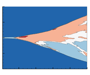
Next, according to the local transition indicator developed above, for the statistically averaged field, the local temporal–spatial transition characteristics can be depicted, as shown in figure 4(b) with contour rendered by different thresholds of $b/b_{nm}$. The deep-blue region is the no-mix (pure fluids) region ($b/b_{nm}=0$), the light-blue region denotes the initial instability region ($b/b_{nm}<(0.2-0.02)$) and the white-like region represents the approximately fully developed turbulence region ($b/b_{nm}\sim 0.2 \pm 0.02$) and the red-like region is the mixing transition region ($b/b_{nm}>0.2+0.02$). It can be seen that the bubble side ($\,y > 0$) transitions first, so that the central turbulence region is closer to the bubble side. On the spike side ($\,y < 0$), it is harder to enter the transition or reach the turbulent state. This is because the spikes are falling faster than the ascending velocity of the bubbles and their speeds can be quite different between different modes, thus harder to reach the self-similar state. All these observations are consistent with our physical understanding.

A comparison with published global transition criteria is also given in figure 4(b). According to Reynolds number ($Re \equiv h\dot h/\nu$, where $h$ and $\dot h$ are the mixing width and its growth rate, and $\nu$ is the kinematic viscosity) criteria, the flow reaches the criterion $1\times 10^{4}$ of Dimotakis (2000) at $t_1=2.61$ ms, and reaches the minimum state turbulence criterion $1.5\times 10^{5}$ of Zhou et al. (2019) at $t_3=9.76$ ms, which represent the global onset of transition and of turbulence, respectively. Meanwhile, according to the integral mixing mass ($M \equiv \int {4\rho {Y_1}} {Y_2}\, {\rm d} V$) criterion of Wang et al. (2022), the flow satisfies the onset of transition condition at $t_2=2.81$ s. It can be seen that the global onsets of transition given by Dimotakis (2000) and Wang et al. (2022) are more backward than that of the local centre position and closer to the peak value of $b/b_{nm}$. At the time of onset of turbulence given by Zhou et al. (2019), for the local flow field, more than $60\,\%$ of the region basically reaches the transition and the turbulent stages.

4. Modelling and validation

4.1. A posteriori validation using LES data

In this section, the present local indicator serves for modifying the gradient transport hypothesis for the turbulent transport terms. The modelling issues related to the eddy viscosity was previously investigated by Livescu et al. (2009) using the high Reynolds number fully resolved numerical simulation of Cabot & Cook (2006). It found that the popular eddy viscosity expression, ${\mu _t} \sim \bar \rho \tilde k/\varepsilon$ ($\tilde k$ and $\varepsilon$ are TKE and dissipation, respectively), does not model the temporal variation of the turbulent transport in any of the moment equations. The results suggest that an eddy viscosity based on a length scale related to the mixing width $h$, ${\mu _t} \sim \bar \rho \sqrt {\tilde k} h$, works well. However, the mixing width is a global quantity and does not lead to local closure. In this paper, based on the present local indicator, we propose a modified eddy viscosity as follows:

(4.1)\begin{equation} {\mu_t} = {C_\mu }\frac{b}{{{\varTheta_b}{b_{nm}}}}\bar \rho \tilde k/\varepsilon, \end{equation}

where ${C_\mu }$ is a model coefficient, chosen such that it yields an optimal match within the mixing layer when $t=10$. Equation (4.1) shows that the results given by the new closure are smaller than those given by the original form in the instability stage (${b}/{{{\varTheta _b}{b_{nm}}}} < 1$), larger in the transition stage (${b}/{{{\varTheta _b}{b_{nm}}}} > 1$) and degenerate to the original form in the fully developed turbulent stage (${b}/{{{\varTheta _b}{b_{nm}}}} \sim 1$). Below, it is shown that the transport terms can be better described using the new closure instead of the original form in the gradient transport hypothesis.

The gradient transport hypothesis for the mass flux is $\overline {\rho '{{u'}_2}} = - ({\mu _t}/{\bar \rho })({{\partial \bar \rho }}/{{\partial {x_2}}})$. Figure 5 plots comparisons of $\overline {\rho '{{u'}_2}}$ across the layer with a gradient transport hypothesis, $- 0.18\tilde k/\varepsilon ({{\partial \bar \rho }}/{{\partial {y}}})$ and $- 0.18({b}/{{{\varTheta _b}{b_{nm}}}})\tilde k/\varepsilon ({{\partial \bar \rho }}/{{\partial {y}}})$ versus $y/W$, at $t=2$ and $t=10$. It clearly shows that the new closure yields better results in the early transition stage, while it gives a similar profile in the later turbulence stage.

Figure 5. Comparisons of $\overline {\rho '{{u'}_2}}$ across the layer with a gradient transport hypothesis, $- 0.18\tilde k/\varepsilon ({{\partial \bar \rho }}/{{\partial {y}}})$ (blue dashed line) and $- 0.18({b}/{{{\varTheta _b}{b_{nm}}}})\tilde k/\varepsilon ({{\partial \bar \rho }}/{{\partial {y}}})$ (red solid line) at $t=2$ (a) and $t=10$ (b). The coefficients are chosen to provide a good fit in the interior of the layer at $t=10$.

The gradient transport hypothesis for the term ${R_{ii2}} \equiv \overline {\rho {{u''}_i}{{u''}_i}{{u''}_2}}$ in kinetic energy equation is ${R_{ii2}}/{\bar \rho } = - ({\mu _t}/{\bar \rho })({{\partial \tilde k}}/{{\partial {x_2}}})$. This term is important both at the centre and edges of the layer (Livescu et al. 2009). As shown in figure 6, the new closure works well both at the transition and turbulence stage, while the standard closure fails to capture the variation in the early transition stage.

Figure 6. Comparison of ${R_{ii2}}/{\bar \rho }$ across the layer with a gradient transport hypothesis, $- 1.0\tilde k/\varepsilon ({{\partial \tilde k }}/{{\partial {y}}})$ (blue dashed line) and $- 1.0({b}/{{{\varTheta _b}{b_{nm}}}})\tilde k/\varepsilon ({{\partial \tilde k }}/{{\partial {y}}})$ (red solid line) at $t=2$ (a) and $t=10$ (b). The coefficients are chosen to provide a good fit in the interior of the layer at $t=10$.

4.2. Modelling validation

In the following part, the improved eddy viscosity is further applied to transition modelling, by coupling with the BHR2 model (Kokkinakis et al. 2019). It should be noticed that much effort has been made to improve the Reynolds-averaged Navier–Stokes (RANS) models’ ability of capturing transition features (Grinstein 2017; Grinstein et al. 2017; Morgan & Black 2019; Singh, Duraisamy & Morgan 2019; Griffond, Soulard & Gréa 2023), including manually controlling the start time of the RANS model (Grinstein 2017), using the hybrid RANS-LES model (Grinstein et al. 2017), developing data-augmented machine learning models (Morgan & Black 2019; Singh et al. 2019), suggesting a new closure of the eddy viscosity model based on the mixing width (Livescu et al. 2009) and proposing a modified dissipation equation to improve the model's transient behaviour (Griffond et al. 2023). Here, the present local transition indicator is used in the closure of the eddy viscosity to characterize the transition process. The governing equations are given by RANS equations. Neglecting mean molecular diffusion, the Favre-averaged continuity, momentum, total energy, species mass fraction and turbulent quantities equations are

(4.2)\begin{gather} \frac{{\partial \bar \rho }}{{\partial t}} + \frac{{\partial \bar \rho {{\tilde u}_j}}}{{\partial {x_j}}} = 0, \end{gather}

(4.3)\begin{gather}\frac{{\partial \bar \rho {{\tilde u}_i}}}{{\partial t}} + \frac{{\partial \bar \rho {{\tilde u}_i}{{\tilde u}_j}}}{{\partial {x_j}}} + \frac{{\partial \bar p}}{{\partial {x_i}}} - \bar \rho {{\bar g}_i} ={-} \frac{{\partial {{\bar \tau }_{ij}}}}{{\partial {x_j}}}, \end{gather}

(4.4)\begin{gather}\frac{{\partial \bar \rho \tilde E}}{{\partial t}} + \frac{{\partial {{\tilde u}_j}( {\bar \rho \tilde E + \bar p} )}}{{\partial {x_j}}} - \bar \rho {{\tilde u}_i}{{\bar g}_i} = \frac{\partial }{{\partial {x_j}}}\left( {\frac{{{\mu_t}}}{{{N_h}}}\frac{{\partial \tilde h}}{{\partial {x_j}}}} \right) + \frac{\partial }{{\partial {x_j}}}\left( {\frac{{{\mu_t}}}{{{N_k}}}\frac{{\partial {{\tilde k}}}}{{\partial {x_j}}} - {{\bar \tau }_{ij}}{{\tilde u}_i}} \right), \end{gather}

(4.5)\begin{gather}\frac{{\partial \bar \rho {{\tilde Y}_a}}}{{\partial t}} + \frac{{\partial \bar \rho {{\tilde u}_j}{{\tilde Y}_a}}}{{\partial {x_j}}} = \frac{\partial }{{\partial {x_j}}}\left( {\frac{{{\mu_t}}}{{{N_Y}}}\frac{{\partial {{\tilde Y}_a}}}{{\partial {x_j}}}} \right), \end{gather}

(4.6)\begin{gather}\frac{{\partial \bar \rho \tilde k}}{{\partial t}} + \frac{{\partial \bar \rho {{\tilde u}_j}\tilde k}}{{\partial {x_j}}} = {C_B}{a_j}\frac{{\partial \bar p}}{{\partial {x_j}}} - {{\bar \tau }_{ij}}\frac{{\partial {{\tilde u}_i}}}{{\partial {x_j}}} + \frac{\partial }{{\partial {x_j}}}\left( {\frac{{{\mu_t}}}{{{N_k}}}\frac{{\partial \tilde k}}{{\partial {x_j}}}} \right) - {C_D}\bar \rho \frac{{{{\tilde k}^{3/2}}}}{{\tilde L}}, \end{gather}

(4.7) \begin{gather}\frac{{\partial \bar \rho \tilde L}}{{\partial t}} + \frac{{\partial \bar \rho {{\tilde u}_j}\tilde L}}{{\partial {x_j}}} = \frac{{\tilde L}}{{\tilde k}}\left[ {\left( {\frac{3}{2} - {C_3}} \right){a_j}\frac{{\partial \bar p}}{{\partial {x_j}}} - \left( {\frac{3}{2} - {C_1}} \right){{\bar \tau }_{ij}}\frac{{\partial {{\tilde u}_i}}}{{\partial {x_j}}}} \right] \!+\! \frac{\partial }{{\partial {x_j}}}\left( {\frac{{{\mu_t}}}{{{N_L}}}\frac{{\partial \tilde L}}{{\partial {x_j}}}} \right) \!+\! {C_L}\bar \rho \sqrt {\tilde k}, \end{gather}

(4.8)\begin{align} \frac{{\partial \bar \rho {a_i}}}{{\partial t}} + \frac{{\partial \bar \rho {{\tilde u}_j}{a_i}}}{{\partial {x_j}}}& = b\frac{{\partial \bar p}}{{\partial {x_i}}} - \frac{{{{\bar \tau }_{ij}}}}{{\bar \rho }}\frac{{\partial \bar \rho }}{{\partial {x_j}}} - {C_{Ba}}\bar \rho {a_j}\frac{{\partial ( {{{\tilde u}_i} - {a_i}} )}}{{\partial {x_j}}} + {C_{Ra}}\bar \rho \frac{{\partial {a_i}{a_j}}}{{\partial {x_j}}} + \frac{\partial }{{\partial {x_j}}}\left( {\frac{{{\mu_t}}}{{{N_a}}}\frac{{\partial {a_i}}}{{\partial {x_j}}}} \right) \nonumber\\ &\quad - {C_{Da}}\bar \rho {a_i}\frac{{\sqrt {\tilde k} }}{{\tilde L}}, \end{align}

(4.9)\begin{align} \frac{{\partial \bar \rho b}}{{\partial t}} + \frac{{\partial \bar \rho {{\tilde u}_j}b}}{{\partial {x_j}}} ={-} 2( {b + 1} ){a_j}\frac{{\partial \bar \rho }}{{\partial {x_j}}} + 2{C_{Rb}}\bar \rho {a_j}\frac{{\partial b}}{{\partial {x_j}}} + {{\bar \rho }^2}\frac{\partial }{{\partial {x_j}}}\left( {\frac{{{\mu_t}}}{{{{\bar \rho }^2}{N_b}}}\frac{{\partial b}}{{\partial {x_j}}}} \right) - {C_{Db}}\bar \rho b\frac{{\sqrt {\tilde k} }}{{\tilde L}},\end{align}

where $\rho$ is the density, $u_i$ is the velocity in the $i$th ($i=1,2,3$) direction, $p$ is the pressure, $g_i$ is the acceleration in the $i$th direction, $E=e+{u_i}^2/2$ is the total energy ($e$ denotes the internal energy), $Y_\alpha$ is the mass fraction of $\alpha$th species. Here $t$ is the temporal coordinate and $x_i$ is the spatial coordinate in the $i$th direction. Based on the BHR2 model framework (Besnard et al. 1992; Rollin et al. 2012; Haines, Grinstein & Schwarzkopf 2013; Denissen et al. 2014; Kokkinakis et al. 2019), four transport equations of turbulent quantities, including the TKE $\tilde k$, the turbulent length scale $\tilde L$, the turbulent mass flux ${a_i} \equiv - \overline {{{u''}_i}}$ and the density-specific-volume covariance $b \equiv - \overline {\rho '{{( {1/\rho } )}^\prime }}$, are introduced.

The right-hand sides of (4.2)–(4.9) are the modelled turbulent terms, in which the turbulent transport terms are described by the gradient diffusion assumption and for the quantity $\phi$,

(4.10)\begin{equation} \frac{{\partial \overline{\rho {{u''}_j}\phi ''} }}{{\partial {x_j}}} ={-} \frac{{{\mu_t}}}{{{N_\phi }}}\frac{{\partial \tilde \phi }}{{\partial {x_j}}}, \end{equation}

where $\mu _t$ is the eddy viscosity and $N_\phi$ is the closure coefficient. Here ${{\bar \tau }_{ij}} \equiv \overline {\rho {{u''}_i}{{u''}_j}}$ is the Reynolds stress, $\tilde h \equiv \tilde e + \bar p/\bar \rho$ is the Favre-averaged enthalpy and $\tilde k \equiv \overline {{{u''}_i}{{u''}_i}} /2$ is the TKE. The equation array is solved by coupling with the equation of state (EOS) $\bar p M =\bar \rho R \tilde T$ for the perfect gas, where $M$ is the molar mass, $R$ is the gas constant and $\tilde T$ is the Favre-averaged static temperature. The assumptions of isotemperature (i.e. $T=T_1=\cdots =T_\alpha$) and partial-pressure (i.e. $p = \sum {{p_\alpha }}$) are used to calculate the EOS of the mixture (Livescu 2013), and the species linearly weighted assumption (i.e. $f = \sum {{Y_\alpha }{f_\alpha }}$) is adopted to calculate the fluid properties of the mixture.

Based on the Boussinesq eddy-viscosity assumption, the Reynolds stress is described as

(4.11)\begin{equation} {{\bar \tau }_{ij}} = \tfrac{2}{3}\bar \rho \tilde k{\delta_{ij}} - 2{\mu_t}( {{{\tilde S}_{ij}} - \tfrac{1}{3}{{\tilde S}_{kk}}{\delta_{ij}}} ), \end{equation}

where ${\tilde S}_{ij}={\frac {1}{2}}({{\partial {{\tilde u}_i}}}/{{\partial {x_j}}} + {{\partial {{\tilde u}_j}}}/{{\partial {x_i}}})$ is the strain-rate tensor. Here, the eddy viscosity is given according to (4.1) as follows:

(4.12)\begin{equation} {\mu_t} = {C_\mu } \frac{b}{{{\varTheta_b}{b_{nm}}}} \bar \rho \sqrt {\tilde k} \tilde L, \end{equation}

where $C_\mu$ is a constant coefficient.

All model coefficients are set according to the work of Kokkinakis et al. (2019). Diffusion coefficients except for $N_K$ and $N_L$ are set to 1.0. Here $N_K$ and $N_L$ are set as 1.1 and 0.125, respectively. Other model coefficients are listed in table 1.

Table 1. Model coefficients for transition modelling.

Then, we apply this model to the RT case and compare it with the LES results. The initial field of 1-D RANS simulation satisfies the isentropic hydrostatic equilibrium, i.e. $\tilde u=0$ and $\bar p/\bar \rho ^\gamma ={\rm const.}$ Combining this with the EOS of the ideal gas, we can integrate the momentum equation to derive the initial profiles of the density and the pressure as follows:

(4.13) \begin{equation} \left.\begin{array}{@{}c@{}} {{\bar \rho }_0}(x) = \left\{ \begin{array}{@{}ll@{}} {{\bar \rho }_{0H}}{\left[ {1 + \dfrac{{\gamma - 1}}{\gamma }\dfrac{{{{\bar \rho }_{0H}}}}{{{{\bar p}_{0I}}}}g(x - {x_I})} \right]^{{1}/({{\gamma - 1}})}} & x < {x_I}\\ {{\bar \rho }_{0L}}{\left[ {1 + \dfrac{{\gamma - 1}}{\gamma } \dfrac{{{{\bar \rho }_{0L}}}}{{{{\bar p}_{0I}}}}g(x - {x_I})} \right]^{{1}/({{\gamma - 1}})}} & x \ge {x_I} \end{array} \right. \\ {{\bar p}_0}(x) = \left\{ \begin{array}{@{}ll} {{\bar p}_{0I}}{\left[ {1 + \dfrac{{\gamma - 1}}{\gamma } \dfrac{{{{\bar \rho }_{0H}}}}{{{{\bar p}_{0I}}}}g(x - {x_I})} \right]^{{\gamma }/({{\gamma - 1}})}} & x < {x_I}\\ {{\bar p}_{0I}}{\left[ {1 + \dfrac{{\gamma - 1}}{\gamma } \dfrac{{{{\bar \rho }_{0L}}}}{{{{\bar p}_{0I}}}}g(x - {x_I})} \right]^{{\gamma }/({{\gamma - 1}})}} & x \ge {x_I} \end{array} \right. \end{array}\right\}, \end{equation}

where ${x_I} = 0$ is the interface position, the subscript 0 denotes the interface (throughout this paper), ${\bar p_{0I}}$ is the interface pressure, ${\bar \rho _{0H}}$ and ${\bar \rho _{0L}}$ denote the density located at $x = {0^- }$ (the side of the heavy fluid) and $x = {0^+ }$ (the side of the light fluid), respectively. Here ${\bar \rho _{0L}}$ is fixed as $1\ {\rm g}\ {\rm cm}^{-3}$, and ${\bar \rho _{0H}}$ is correspondingly set as ${\bar \rho _{0H}} = {\bar \rho _{0L}}(1+A_t)/(1-A_t)\ {\rm g}\ {\rm cm}^{-3}$. The value of ${\bar p_{0I}}$ will influence the shape of the density profile, and a larger value of ${\bar p_{0I}}=6000\ {\rm g} {\rm cm}^{-1}\ {\rm s}^{-2}$ is used to lead to a flatter density profile to approach incompressible limit. The velocity is initialized as zero across the whole field. The mass fraction of heavy fluid ${\tilde Y_1}(x)$ is set as 1 for $x < {x_I}$ and 0 for $x \ge {x_I}$. Inside the perturbed region($|x| \le \Delta x$, $\Delta x$ is the mesh scale), ${\tilde k}(0)$ is set as ${\tilde k}(0) = A_tg\tilde L(0)$ by a simple dimensional analysis, $\tilde L(0)$ is the initial length scale and is set as $\tilde L(0) = 1 \times {10^{ - 3}}$, initial mass flux $a_x(0)$ is set to $\sqrt {\tilde k( 0 )} /4$, $b(0)$ is initialized as a small value of $10^{-8}$ (Kokkinakis et al. 2019). The boundaries at the start and the end of the computational domain are set as wall conditions.

A grid convergence study is performed for the present BHR2 model using three grids composing of 300, 600 and 1200 cells, as shown in figure 7. For grid resolutions of 300, discrepancies are observed between the predicted bubble height $h_b$ and maximum TKE $K_{max}$ when compared with grid resolutions of 600 during the early stages. Nevertheless, the model exhibits clear grid convergence behaviour from 600 to 1200 cells. Consequently, all subsequent results showcased are computed using a grid resolution of 600.

Figure 7. Temporal evolution of the bubble height $h_b$ versus self-similar time $A_t g t^2$ (a) and the maximum TKE $K_{max}$ versus $t$ (b) for RT mixing using the present BHR2 model: effect of grid resolution.

Figure 8 shows comparisons of temporal evolutions of the bubble height $h_b$ and its growth rate $\alpha _b$ versus self-similar time $A_t g t^2$ among LES, the BHR2 model and the present BHR2 model with transition. The results suggest that both turbulence models enter the quadratic growth stage earlier as compared with the results of LES, and their growth rates saturate to the same value of 0.043. This discrepancy occurs because the initial set of LES incorporates long-wavelength perturbation, consequently elongating the transitional stage. Investigating how to tailor the turbulence model's initial conditions to encompass the spectral properties of these perturbations presents a subject conducive to further study. It is noticed that the present model, owing to its consideration of transition effects, displays a smaller overall mixing width development than the BHR2 model, aligning more closely with the LES.

Figure 8. Comparisons of temporal evolutions of the bubble height $h_b$ (a) and its growth rate $\alpha _b$ (b) versus self-similar time $A_t g t^2$ among LES (black circles), BHR2 model (blue solid lines) and the present BHR2 model with transition (red solid lines). Legends of the following figures are the same as this.

Figure 9 further depicts comparisons of temporal evolutions of the maximum TKE $K_{max}$ and the maximum density specific volume covariance $b_{max}$ versus time $t$. It illustrates that the present model exhibits better agreement with LES results in the early stage, while the BHR2 model tends to overestimate the TKE and $b$ due to its neglect of transition effects. In the late stage, the evolution characteristics of both models converge to a similar behaviour, e.g. the $b_{max}$ saturates to a constant value of $0.2b_{nm}^{max }$ in agreement with the LES results.

Figure 9. Comparisons of temporal evolutions of the maximum TKE $K_{max}$ (a) and the maximum density specific volume covariance $b_{max}$ (b) versus time $t$.

Moreover, the predicted profiles of turbulent transport $\overline {\rho 'u'}$, ${{{R_{ii2}}}}/{{\bar \rho }}$, VF $\tilde f$, TKE $\tilde k$, mass flux $a_x$ and density specific volume covariance $b$ are shown in figures 10 and 11 for $t=10$ and $t=2$, respectively. It is noteworthy to clarify that the 1-D RANS simulations in this study are conducted solely in the $x$-direction, with the acceleration aligned along the $x$-axis as well. The heavy fluid is positioned to the left of the domain ($x<0$). Conversely, for the 3-D LES, the acceleration is oriented along the $y$-axis, and the heavy fluid is situated on the right-hand side of the domain ($y>0$). Consequently, when comparing the RANS and LES results, the LES results necessitate a coordinate transformation to align with the RANS reference frame, wherein $-y$ corresponds to the $x$-coordinate, and physical quantities such as $\overline {\rho 'u'}$, ${{{R_{ii2}}}}/{{\bar \rho }}$, mass flux $a_x$ require a sign reversal for an apt comparison. Accordingly, subsequent figures presented will adhere to the coordinate system and scaling of the 1-D RANS simulations, depicting $x/W$ as the horizontal axis. In comparison to figures 5 and 6, profile plots of the physical quantities $\overline {\rho 'u'}$ and ${{{R_{ii2}}}}/{{\bar \rho }}$ necessitate not only a transformation of the abscissa polarity (from positive to negative or vice versa) but also an inversion of the magnitude of these physical quantities. This ensures a consistent comparison between the LES and RANS results. In the late turbulent stage ($t=10$), both RANS models exhibit commendable predictive capabilities, with the present model demonstrating a closer agreement with LES results in terms of magnitude. In the early transition stage ($t=2$), the modified model's predictions are not as large as those of the unmodified BHR2 model, as they are compared through posterior analysis in § 4.1. Instead, they are found to be smaller. This disparity can be attributed to the fact that in the posterior analysis, all results are derived based on accurate LES data directly applied to the target quantities of interest. Conversely, the RANS predictions might encompass inaccuracies due to the potentially suboptimal treatment of individual physical quantities and their strong interdependencies. Note that the introduced local transition indicator contributes to the turbulent viscosity term, thereby influencing the computation of Reynolds stresses and diffusion terms. However, considering that for RT turbulent mixing, the dominant production mechanism is driven by buoyancy effects rather than shear effects. Thus, the modification in transition modelling does not fundamentally alter the production–dissipation balance, resulting in the primary characteristics and growth rates remaining consistent with the unmodified model. There remains considerable scope for further research and improvement in effectively incorporating the local transition indicator within the BHR2 model to enhance the capturing of transition features.

Figure 10. Comparisons of profiles of turbulent transport $\overline {\rho 'u'}$, ${{{R_{ii2}}}}/{{\bar \rho }}$, VF $\tilde f$, TKE $\tilde k$, mass flux $a_x$ and density specific volume covariance $b$ at $t=10$.

Figure 11. Comparisons of profiles of turbulent transport $\overline {\rho 'u'}$, ${{{R_{ii2}}}}/{{\bar \rho }}$, VF $\tilde f$, TKE $\tilde k$, mass flux $a_x$ and density specific volume covariance $b$ at $t=2$.

5. Conclusion

In this paper, a new perspective on the local transition indicator and modelling of turbulent mixing is proposed. That is, from the point of view of fusion engineering applications, developing a local transition indicator based on the mixing state. This indicator is employed using LES of RT turbulent mixing and compared with established global criteria. So far as we know, this is the first time that the local spatiotemporal transition characteristics of turbulent mixing are depicted.

Furthermore, the present indicator is validated by investigating the modelling issues of the gradient transport hypothesis. The analysis of the LES results proves that a new closure of eddy viscosity based on the transition indicator provides a reasonably good description of the transport terms both in transition and turbulence stages. Thus, we further apply this local transition indicator for transition modelling, by coupling it with the BHR2 model. Note that predictions in the late stage exhibit better agreement with LES data; there remains substantial room for improvement in predictions of the transition stage. The refinement of methodologies to better incorporate the employment of the local transition indicator into the BHR2 model for more accurately capturing transition characteristics warrants further investigation. Notice that $b$ is related to the mixing state, whose evolution substantially depends on the initial perturbed spectrum. This model may have better sensitivity to the mixing transition process induced by different initial disturbances. This endeavour is expected to contribute to the understanding and simulation of complex fusion scenarios, especially for precise calculations of reaction rates and assessments of fusion performance.

However, before embarking on practical applications in fusion engineering, several challenges need to be addressed. Primarily, it is crucial to assess the model's adaptability to complex mixing problems, like reshocked RM and spherical implosion issues. This might involve refining the local transition criterion's asymptotic value of 0.2 and addressing realizable concerns. Additionally, enhancing the description accuracy of mixing state representation necessitates incorporating the dynamics of particles and their interaction with turbulence. Integrating a particle-turbulence framework into the transition modelling could lead to a more comprehensive understanding and predictive capability. These upcoming tasks, while posing their own complexities, offer exciting opportunities for further refining the local transition indicator and solidifying its position as a powerful tool in fusion engineering. Future publications are awaited to chronicle these advancements.