Hostname: page-component-745bb68f8f-cphqk Total loading time: 0 Render date: 2025-01-27T11:43:32.828Z Has data issue: false hasContentIssue false

Bounding heat transport in supergravitational turbulent thermal convection

Published online by Cambridge University Press:  19 December 2024
Zijing Ding*
Affiliation:
Institute of Mechanics, Chinese Academy of Sciences, Beijing 100190, PR China School of Energy Science and Engineering, Harbin Institute of Technology, Harbin 150001, PR China
*
Email address for correspondence: [email protected]

Abstract

This paper derives the upper bound on heat transport in supergravitational turbulent thermal convection analytically and numerically. Using a piecewise background profile, the functional inequality analysis delivers a suboptimal bound $Nu\lesssim -({3\sqrt {3}}/{2})({\eta \ln (\eta )}/({1-\eta ^2}))\,Ra^{1/2}$ as $Ra\rightarrow \infty$, where $Nu$ is the Nusselt number, $\eta$ is the radius ratio of the inner cylinder to the outer cylinder ($0<\eta <1$), and $Ra$ is the Rayleigh number. A variational problem yielded from Doering–Constantin–Hopf formalism is solved asymptotically and numerically, which delivers a better upper bound than the piecewise background profile. The asymptotic analysis and numerical data indicate that the current best bound is given by $Nu\leqslant -0.106({\eta \ln (\eta )}/({(1-\eta )(1+\sqrt {\eta })^2}))\,Ra^{1/2}$. Both analytical and numerical results demonstrate that the upper bound can be significantly reduced by the curvature effect. Unlike the traditional Rayleigh–Bénard turbulence, in which the optimal perturbation yielded from the variational problem is always two-dimensional, the present study shows that three-dimensional perturbations, annular perturbations and axisymmetric perturbations can be induced by the curvature effect simultaneously. However, we show that the bound yielded from the three-dimensional variational problem is very close to the axisymmetric situation as $\eta$ increases and $Ra$ increases.

Type
JFM Papers
Copyright
© The Author(s), 2024. Published by Cambridge University Press

1. Introduction

The Rayleigh–Bénard convection between two parallel plates has been the paradigm for exploring the scaling laws in thermal turbulence as the driving parameter approaches infinity (Ahlers, Grossmann & Lohse Reference Ahlers, Grossmann and Lohse2009; Lohse & Xia Reference Lohse and Xia2010; Ecke & Shishkina Reference Ecke and Shishkina2023; Lindborg Reference Lindborg2023). A classical scaling law for heat transport proposed by Malkus (Reference Malkus1954) is still competing with the ‘ultimate scaling’, which was proposed by Kraichnan (Reference Kraichnan1962). Experiments and current direct numerical simulations (DNS) seem to support the classical scaling (Urban, Musilová & Skrbek Reference Urban, Musilová and Skrbek2011; Bouillaut et al. Reference Bouillaut, Lepot, Aumaître and Gallet2019; Iyer et al. Reference Iyer, Scheel, Schumacher and Sreenivasan2020). But there are some competing claims of the existence of ultimate scaling (He et al. Reference He, Funfschilling, Nobach, Bodenschatz and Ahlers2012; Zhu et al. Reference Zhu, Mathai, Stevens, Verzicco and Lohse2018). The debate over the classical and ultimate scalings stems from two factors: it is difficult to push the driving parameter higher but keep the other parameters constant in experiments; and the formidable DNS are limited by current computational power.

Recently, Sun and his collaborators proposed a novel experimental study of thermal turbulence between two co-rotating cylinders (Jiang et al. Reference Jiang, Zhu, Wang, Huisman and Sun2020, Reference Jiang, Wang, Liu and Sun2022), in which the non-Oberbeck–Boussinesq effects are negligible. The inner cylinder is cooled while the outer cylinder is heated, while they are rotating at the same angular speed. The centrifugal force can drive turbulent convection more efficiently than buoyancy in traditional Rayleigh–Bénard convection, which is referred to as supergravitational convection. Jiang et al. (Reference Jiang, Wang, Liu and Sun2022) reported that transition to the ultimate regime in the supergravitational convection occurs at $Ra\sim 10^{11}$ (where $Ra$ is the Rayleigh number). They observed the scaling $Nu\sim Ra^{0.4}$ in the range $Ra\in [10^{11},4\times 10^{12}]$ (where $Nu$ is the Nusselt number, measuring the ratio between total heat transport and that by pure conduction), which is clearly higher than Malkus's classical scaling. Wang et al. (Reference Wang, Jiang, Liu, Zhu and Sun2022) further examined the influence of curvature on the heat transfer, and reported that heat transfer is generally inhibited by curvature, and Zhong, Wang & Sun (Reference Zhong, Wang and Sun2023) investigated the influence of an imposed shear flow on the heat transfer. However, Wang et al. (Reference Wang, Jiang, Liu, Zhu and Sun2022) focused on relatively lower $Ra$ flow, and they did not give an analytical expression for the geometrical dependence. Moreover, there is no report on curvature's influence on the ultimate regime scaling. In addition, it would be interesting to ask if the supergravitational convection can transport more heat beyond Kraichnan's scaling.

A potential way to provide insights into the above questions is to derive an upper bound on heat transfer in supergravitational convection. The upper bound is usually derived from a variational problem, which has its root in Malkus (Reference Malkus1954). Turbulence was hypothesized to maximize heat transfer in traditional Rayleigh–Bénard convection, resulting in a maximization problem (Howard Reference Howard1963; Busse Reference Busse1969). A multi-$\alpha$ technique was used to solve the maximization problem, which was very tedious. A complementary minimization problem was proposed by Doering & Constantin (Reference Doering and Constantin1996), which was built upon the so-called background field method. The background field method is also referred to as Doering–Constantin–Hopf formalism (Wen et al. Reference Wen, Chini, Kerswell and Doering2015), which has a superb advantage compared to the maximization problem because it can yield an upper bound even for a trial background field. The current best upper bound on traditional Rayleigh–Bénard convection for arbitrary Prandtl number ($Pr$) yielded from Doering–Constantin–Hopf formalism was delivered by Plasting & Kerswell (Reference Plasting and Kerswell2003). Ding & Kerswell (Reference Ding and Kerswell2020) proved that it is impossible to improve (lower) the upper bound by considering a high-dimensional background field. Note that the upper bound given by Plasting & Kerswell (Reference Plasting and Kerswell2003) (${\sim }Ra^{1/2}$) is actually much higher than in the DNS and experimental data (${\sim }Ra^{1/3}$) since it uses only partial information from equations of motion. The $1/2$ scaling can be improved (lowered) if more constraints from equations of motion can be imposed. For instance, Whitehead & Doering (Reference Whitehead and Doering2011), Wen et al. (Reference Wen, Chini, Kerswell and Doering2015) and Ding & Wen (Reference Ding and Wen2020) showed that the bound can be lowered to ${\sim }Ra^{5/12}$ in two-dimensional (2-D) traditional Rayleigh–Bénard convection with stress-free boundary conditions when the vorticity equation is added as an additional constraint. When the Prandtl number is infinity, more constraints can be derived from the Stokes equations, and the bound on heat transport in traditional Rayleigh–Bénard convection between no-slip walls can be improved to $Ra^{1/3}$ with logarithmic corrections (Plasting & Ierley Reference Plasting and Ierley2005; Ierley, Plasting & Kerswell Reference Ierley, Plasting and Kerswell2006; Otto & Seis Reference Otto and Seis2011). Choffrut, Nobili & Otto (Reference Choffrut, Nobili and Otto2016) proved that the $1/3$ scaling with logarithmic correction is also the upper bound for finite but large Prandtl number flows as $Pr\geqslant (Ra\ln (Ra))^{1/3}$. In this study, we aim to derive an upper bound on heat transport in supergravitational convection of arbitrary Prandtl number. The influence of the geometry, i.e. the radius ratio, on the upper bound will be examined. It will be interesting to explore if an analytical expression of geometrical dependence can be derived.

Usually, the analytical result for an upper bound can be derived from the functional inequality analysis (Doering & Constantin Reference Doering and Constantin1996; Whitehead & Doering Reference Whitehead and Doering2011; Ding & Wen Reference Ding and Wen2020; Kumar Reference Kumar2022). Two different routes can be used to find the analytical upper bound: a direct method proposed by Seis (Reference Seis2015), and an auxiliary functional method by Chernyshenko et al. (Reference Chernyshenko, Goulart, Huang and Papachristodoulou2014). Their relationship is established by Chernyshenko (Reference Chernyshenko2022). The direct method does not apply the background field decomposition, while the quadratic auxiliary functional method is equivalent to the Constantin–Doering–Hopf formalism (Chernyshenko et al. Reference Chernyshenko, Goulart, Huang and Papachristodoulou2014; Rosa & Temam Reference Rosa and Temam2022). Indeed, Chernyshenko (Reference Chernyshenko2022) showed that the direct method and background field method can yield same analytical upper bound. In the present work, we will apply the Constantin–Doering–Hopf formalism to derive the analytical bound. However, the functional inequality analysis of the Constantin–Doering–Hopf formalism often delivers a suboptimal bound, and the best upper bound can be obtained only by solving an Euler–Lagrange system that ensued from Constantin–Doering–Hopf formalism numerically. But numerical solution cannot deliver an analytical expression for the geometrical dependence. Kumar (Reference Kumar2022) showed that in Taylor–Couette flow, an analytical expression of geometrical dependence can be obtained by solving a one-dimensional Euler–Lagrange system. This inspires us to examine if the Kumar (Reference Kumar2022) approach can be extended to the present supergravitational convection. Furthermore, it will be interesting to examine if the DNS data by Wang et al. (Reference Wang, Jiang, Liu, Zhu and Sun2022) follow the analytical geometrical dependence once it is obtained.

Hence this paper is organized as follows. Section 2 formulates the upper bound problem of supergravitational convection. An analytical suboptimal bound is derived using a piecewise background field in § 3. The Euler–Lagrange equations that ensued from the upper bound problem are presented in § 4. A one-dimensional version of the Euler–Lagrange equations is solved asymptotically in § 4.1 by dropping the constraint of the continuity equation, which delivers an analytical expression of geometrical dependence for the upper bound in supergravitational convection. Fully numerical results for the Euler–Lagrange equations are presented in § 4.2. Comparison with the DNS data by Wang et al. (Reference Wang, Jiang, Liu, Zhu and Sun2022) is made in § 4.3. Discussion and conclusion are given in § 5.

2. Mathematical formulation of the upper bound problem

2.1. Governing equations

We consider an annular liquid layer bounded by two infinitely long concentric co-rotating cylinders with constant angular speed $\omega$. The inner cylinder is of radius $R_i$, and the outer cylinder is of radius $R_o$. The liquid is Newtonian of constant kinematic viscosity $\nu$ and thermal diffusivity $\kappa$. A high temperature $T_o$ is imposed on the outer cylinder, while a lower temperature $T_i$ is imposed on the inner cylinder. Using the same scales for length ($d=R_o-R_i$), velocity (free-fall velocity is $U=\sqrt {\alpha \omega ^2(R_o+R_i)d/2}$, and $\alpha$ is the thermal expansion coefficient), pressure ($\rho U^2$) and temperature ($\Delta T=T_o-T_i$) as in Jiang et al. (Reference Jiang, Zhu, Wang, Huisman and Sun2020, Reference Jiang, Wang, Liu and Sun2022) and Wang et al. (Reference Wang, Jiang, Liu, Zhu and Sun2022), we start from the dimensionless governing equations of the supergravitational convection (Wang et al. Reference Wang, Jiang, Liu, Zhu and Sun2022):

(2.1)$$\begin{gather} \boldsymbol{\nabla}\boldsymbol{\cdot}\boldsymbol{u}=0, \end{gather}$$
(2.2)$$\begin{gather}\partial_t\boldsymbol{u}+\boldsymbol{u}\boldsymbol{\cdot}\boldsymbol{\nabla}\boldsymbol{u}+Ro^{{-}1}\,\boldsymbol{u}\times\omega\,\boldsymbol{e}_z+\boldsymbol{\nabla}p- \sqrt{\frac{Pr}{Ra}}\,\nabla^2\boldsymbol{u}+2\,\frac{1-\eta}{1+\eta}\,Tr\,\boldsymbol{e}_r=\boldsymbol{0}, \end{gather}$$
(2.3)$$\begin{gather}\partial_tT+\boldsymbol{u}\boldsymbol{\cdot}\boldsymbol{\nabla}T-\frac{1}{\sqrt{Pr\,Ra}}\,\nabla^2T=0, \end{gather}$$

where $\boldsymbol {u}=u\boldsymbol {e}_r+v\boldsymbol {e}_\phi +w\boldsymbol {e}_z$ is the velocity, $T$ is the temperature, $Pr=\nu /\kappa$ is the Prandtl number, $Ra=\alpha \omega ^2(R_i+R_o)\,\Delta T\,d^3/(2\nu \kappa )$ is the Rayleigh number, $Ro=\sqrt {\alpha \,\Delta T\,(R_i+R_o)/(2d)}/2$ is the Rossby number, and $\eta =R_i/R_o$ ($0<\eta <1$) is the radius ratio.

There is no slip or penetration at the inner and outer cylinders:

(2.4)\begin{equation} \boldsymbol{u}=\boldsymbol{0}\quad \textrm{at}\ r=R_i/d=r_i, r=R_o/d=r_o. \end{equation}

Note that $r_i=\eta /(1-\eta )$ and $r_o=1/(1-\eta )$.

The dimensionless temperatures at the cylinders are

(2.5a,b)\begin{equation} T=0 \textrm{ at}\ r=r_i,\quad T=1 \textrm{ at}\ r=r_o. \end{equation}

2.2. The Nusselt number

We define a temporal-surface average as

(2.6)\begin{equation} \bar{\bullet}=\lim_{t^*\rightarrow\infty\atop\\ L\rightarrow\infty}\frac{1}{2{\rm \pi} Lt^*}\int^{t^*}_0\int^{L/2}_{{-}L/2}\int^{2{\rm \pi}}_0 \bullet \,\textrm{d}\phi \,\textrm{d}z\,\textrm{d}t. \end{equation}

Then the temporal-volume average is defined as

(2.7)\begin{equation} \langle\bullet\rangle=\frac{2}{r_o^2-r_i^2}\int^{r_o}_{r_i}r\,\bar{\bullet} \,\textrm{d}r. \end{equation}

Taking the temporal-surface average on the thermal equation (2.3), we obtain

(2.8)\begin{equation} \frac{\textrm{d}}{\textrm{d} r}\left(r\,\frac{\textrm{d}\bar{T}}{\textrm{d}r}-\sqrt{Pr\,Ra}\,r\,\overline{uT}\right)=0. \end{equation}

Hence the total heat flux is defined as

(2.9)\begin{equation} J=r\,\frac{\textrm{d}\bar{T}}{\textrm{d}r}-r\,\sqrt{Pr\,Ra}\,\overline{uT}. \end{equation}

The heat flux $J$ is thus independent of $r$ as $\textrm{d}J/\textrm{d}r=0$. At the conduction state, we have $J_{con}=-1/\ln (\eta )$.

To quantify the heat flux, the Nusselt number $Nu$ can be defined as

(2.10)\begin{equation} Nu=\frac{J}{J_{con}}=\frac{r\,\dfrac{\textrm{d}\bar{T}}{\textrm{d}r}-r\,\sqrt{Pr\,Ra}\,\overline{uT}}{J_{con}}. \end{equation}

Multiplying by $r$ on both sides of (2.10) and integrating over the domain $r\in [r_i,r_o]$ yields

(2.11)\begin{equation} Nu=\ln(\eta)\,\langle \sqrt{Pr\,Ra}\,ruT-r\,\partial_rT\rangle. \end{equation}

Multiplying by $T$ in the thermal equation (2.3) and taking the temporal-volume average of it gives

(2.12)\begin{equation} \frac{r_o^2-r_i^2}{2}\,\langle|\boldsymbol{\nabla} T|^2\rangle=\left.r\,\frac{\textrm{d}\bar{T}}{\textrm{d}r}\right|_{r=r_o}, \end{equation}

where the boundary conditions of $\boldsymbol {u}$ and $T$ at the two walls are used. Note that $r({\textrm{d}\bar {T}}/{\textrm{d}r})|_{r=r_o}$ is the thermal flux $J$ at the outer cylinder. Hence the Nusselt number $Nu$ can also be defined as

(2.13)\begin{equation} Nu=\frac{r_o^2-r_i^2}{2}\,\frac{\langle|\boldsymbol{\nabla} T|^2\rangle}{J_{con}}. \end{equation}

The Nusselt number is the key quantity to be investigated in the present work, and we are going to explore the upper bound on $Nu$ and its dependence on $\eta$ and $Ra$.

2.3. The background method

Now we apply the background method and decompose the temperature field as follows:

(2.14)\begin{equation} T=\tau(r)+\theta. \end{equation}

Here, we assumed that the background velocity field is zero while the background temperature $\tau$ is one-dimensional. The background field $\tau$ carries the boundary conditions of $T$ at $r=r_i$, $r_o$, while the perturbation field $\theta$ satisfies the homogeneous boundary conditions. Ding & Kerswell (Reference Ding and Kerswell2020) showed that a one-dimensional background field is the optimal choice for traditional Rayleigh–Bénard convection. In fact, the zero background velocity field can be established using symmetry reduction (Fantuzzi, Arslan & Wynn Reference Fantuzzi, Arslan and Wynn2022): the solution should be invariant in azimuthal ($\phi$) and axial ($z$) directions under a ‘flow reversal operation’.

Substituting the background decomposition (2.14) into the momentum equation (2.2) and heat equation (2.3) gives

(2.15)$$\begin{gather} \boldsymbol{M}:=\partial_t\boldsymbol{u}+\boldsymbol{u}\boldsymbol{\cdot}\boldsymbol{\nabla}\boldsymbol{u}+Ro^{{-}1}\,\boldsymbol{u} \times\omega\,\boldsymbol{e}_z+\boldsymbol{\nabla}p-\sqrt{\frac{Pr}{Ra}}\,\nabla^2\boldsymbol{u}+2\, \frac{1-\eta}{1+\eta}\,(\tau(r)+\theta)r\,\boldsymbol{e}_r=\boldsymbol{0}, \end{gather}$$
(2.16)$$\begin{gather}{H}:=\partial_t\theta+\boldsymbol{u}\boldsymbol{\cdot}\boldsymbol{\nabla}\theta+u\,\frac{\textrm{d}\tau}{\textrm{d}r}-\frac{1}{\sqrt{Pr\,Ra}}\,\nabla^2\theta-\frac{1}{\sqrt{Pr\,Ra}}\left(\frac{\textrm{d}^2\tau}{\textrm{d}r^2}+\frac{1}{r}\,\frac{\textrm{d}\tau}{\textrm{d}r}\right)=0. \end{gather}$$

Dotting $\boldsymbol {u}$ on the momentum equation (2.15) and taking the temporal-volume average on it gives the kinetic energy balance constraint

(2.17)\begin{equation} \sqrt{\frac{Pr}{Ra}}\,\langle |\boldsymbol{\nabla}\boldsymbol{u}|^2\rangle+2\,\frac{1-\eta}{1+\eta}\,\langle r(\tau+\theta)u\rangle=0. \end{equation}

Multiplying $\theta$ on the heat equation (2.16) and taking the temporal-volume average on it gives the thermal energy balance condition

(2.18)\begin{equation} \left\langle \frac{1}{\sqrt{Pr\,Ra}}\,|\boldsymbol{\nabla}\theta|^2+u\theta\,\frac{\textrm{d}\tau}{\textrm{d}r}+\frac{1}{\sqrt{Pr\,Ra}}\,\frac{\textrm{d}\tau}{\textrm{d}r}\,\frac{\partial\theta}{\partial r}\right\rangle=0. \end{equation}

We also rewrite the definitions of Nusselt number (2.10) and (2.11) using the background field decomposition:

(2.19)$$\begin{gather} Nu=\ln(\eta)\,\langle \sqrt{Pr\,Ra}\,ru(\theta+\tau)-r\,\partial_r(\tau+\theta)\rangle, \end{gather}$$
(2.20)$$\begin{gather}Nu=\frac{r_o^2-r_i^2}{2}\,\frac{\langle|\boldsymbol{\nabla} T|^2\rangle}{J_{con}}={-}\ln(\eta)\,\frac{r_o^2-r_i^2}{2}\,\langle|\boldsymbol{\nabla}(\theta+\tau)|^2\rangle. \end{gather}$$

Now we can combine the constraints (2.17)–(2.18) together with the definition of $Nu$ in (2.20):

(2.21)\begin{align} {-}\frac{Nu}{\ln(\eta)}&=\frac{r_o^2-r_i^2}{2}\left\{\langle |\boldsymbol{\nabla} (\theta+\tau)|^2\rangle-a\,\sqrt{Pr\,Ra}\left(\sqrt{\frac{Pr}{Ra}}\,\langle |\boldsymbol{\nabla}\boldsymbol{u}|^2\rangle+2\,\frac{1-\eta}{1+\eta}\,\langle r(\tau+\theta)u\rangle\right)\right.\nonumber\\ &\quad\left. {}-2{b}\,\sqrt{Pr\,Ra}\left\langle \frac{1}{\sqrt{Pr\,Ra}}\,|\boldsymbol{\nabla}\theta|^2+u\theta\,\frac{\textrm{d}\tau}{\textrm{d}r}+\frac{1}{\sqrt{Pr\,Ra}}\,\frac{\textrm{d}\tau}{\textrm{d}r}\,\frac{\partial\theta}{\partial r}\right\rangle\right\}. \end{align}

The free parameter $a$ is to impose the energy balance condition, and the free parameter $b$ is to impose the balance of heat flux (Ding & Wen Reference Ding and Wen2020). However, Ding & Wen (Reference Ding and Wen2020) showed that including the free parameter $b$ improves the prefactor of the upper bound only very slightly in the classical Rayleigh–Bénard convection (less than $1\,\%$). Hence in the present work, we follow Whitehead & Doering (Reference Whitehead and Doering2011) and Wen et al. (Reference Wen, Chini, Kerswell and Doering2015), and choose to fix $b=1$, which simplifies the computation of the bound. Fixing $b=1$, however, means that our background field formulation is no longer optimal.

Using (2.19), we can eliminate the term $(({1-\eta })/({1+\eta }))\langle r(\tau +\theta )u\rangle$ in (2.21):

(2.22) \begin{align} -\frac{Nu}{\ln(\eta)}&=\int^{r_o}_{r_i}r\left(\frac{\textrm{ d}\tau}{\textrm{d}r}\right)^2\,\textrm{ d}r-a\,\frac{r_o^2-r_i^2}{2}\nonumber\\ &\quad \times \left(Pr\,\langle |\boldsymbol{\nabla}\boldsymbol{u}|^2\rangle+2\,\frac{1-\eta}{1+\eta}\left(\frac{Nu}{\ln(\eta)}+\left\langle r\,\frac{\partial(\theta+\tau)}{\partial r}\right\rangle\right)\right)\nonumber\\ &\quad -\frac{r_o^2-r_i^2}{2}\left\langle2\,\sqrt{Pr\,Ra}\,\theta u\,\frac{\textrm{ d}\tau}{\textrm{ d}r}+|\boldsymbol{\nabla}\theta|^2\right\rangle. \end{align}

Note that $(r_o^2-r_i^2)(({1-\eta })/({1+\eta }))=1$ when substituting $r_o=1/(1-\eta )$ and $r_i=\eta /(1-\eta )$ into this term.

Rearranging (2.22) gives the equation

(2.23)\begin{equation} {-}\frac{Nu}{\ln(\eta)}=\frac{1}{1-a}\int_{r_i}^{r_o} r\left(\frac{\textrm{d}\tau}{\textrm{d}r}\right)^2-2a\,\frac{1-\eta}{1+\eta}\,r^2\,\frac{\textrm{d}\tau}{\textrm{d}r}\,\textrm{d}r-\frac{1}{1-a}\,\mathscr{G}, \end{equation}

where

(2.24)\begin{equation} \mathscr{G}:=\frac{r_o^2-r_i^2}{2}\left\langle a\,Pr\,|\boldsymbol{\nabla}\boldsymbol{u}|^2+|\boldsymbol{\nabla}\theta|^2+2\,\sqrt{Pr\,Ra}\,\theta u\,\frac{\textrm{d}\tau}{\textrm{d}r}+\underbrace{2a\,\frac{1-\eta}{1+\eta}\,r\,\frac{\partial\theta}{\partial r}}_{linear\ term}\right\rangle. \end{equation}

Hence for $0< a<1$, the upper bound on $-Nu/\ln (\eta )$ is given by

(2.25)\begin{equation} {-}\frac{Nu}{\ln(\eta)}\le\frac{1}{1-a}\int^{r_o}_{r_i} r\left(\frac{\textrm{d}\tau}{\textrm{d}r}\right)^2-2a\,\frac{1-\eta}{1+\eta}\,r^2\,\frac{\textrm{d}\tau}{\textrm{d}r}\,\textrm{d}r-\frac{1}{1-a}\min_{\boldsymbol{u},\theta\, {s.t.}\,{BCs}\atop \boldsymbol{\nabla}\boldsymbol{\cdot}\boldsymbol{u}=0}\mathscr{G}, \end{equation}

where ‘BCs’ stands for boundary conditions of $\boldsymbol {u}$ and $\theta$. The linear term in $\mathscr {G}$ can be removed by defining the following shifted fluctuation field:

(2.26a,b)\begin{equation} \boldsymbol{u}=0+\hat{\boldsymbol{u}},\quad \theta={-}\frac{a}{2}\,\frac{1-\eta}{1+\eta}\,(r^2-r_i^2)-\frac{a}{2\ln(\eta)}\ln(r/r_i)+\hat{\theta}, \end{equation}

in which $\bar {\hat {\boldsymbol {u}}}=\bar {\hat {\theta }}=0$. We take this shift because the linear term in $\mathscr {G}$ will cause a non-zero contribution to $({1}/({1-a}))\int ^{r_o}_{r_i} r({\textrm{d}\tau }/{\textrm{d}r})^2-2a(({1-\eta })/({1+\eta }))r^2({\textrm{d}\tau }/{\textrm{d}r})\,\textrm{d}r$ in (2.25). This particular shift can be sought by constructing a minimization problem for $\mathscr {G}$ (see Appendix A).

By using the shifted fluctuations, we rewrite $\mathscr {G}$ as

(2.27)\begin{equation} \mathscr{G}=\frac{r_o^2-r_i^2}{2}\,\mathscr{H}-\frac{a^2}{4}\left(\frac{1}{1+\eta}+r_i+\frac{1}{\ln(\eta)}\right), \end{equation}

where

(2.28)\begin{equation} \mathscr{H}=\left\langle a\,Pr\,|\boldsymbol{\nabla}\boldsymbol{u}|^2+|\boldsymbol{\nabla}\theta|^2+2\,\sqrt{Pr\,Ra}\,\theta u\,\frac{\textrm{d}\tau}{\textrm{d}r}\right\rangle. \end{equation}

Here, we drop the hat on $\theta$ and $\boldsymbol {u}$ for simplicity; and if we rescale the velocity $\boldsymbol {u}$ by defining $\sqrt {Pr}\,\boldsymbol {u}=\boldsymbol {u}^*$, then the Prandtl number will not appear in $\mathscr {H}$. Thus the Prandtl number does not affect the bound in supergravitational convection. This is so because we are interested only in the minimum of $\mathscr {H}$ over a linear space of velocity and temperature fields, and the rescaling amounts to a reparametrization of the optimization variables that does not affect the upper bound on $Nu$. Now the upper bound on $-Nu/\ln (\eta )$ can be stated as

(2.29)\begin{equation} {-}\frac{Nu}{\ln(\eta)}\leqslant nu-\frac{1}{1-a}\min_{\boldsymbol{u},\theta\, \textit{s.t.}\,\textit{BCs}\atop \boldsymbol{\nabla}\boldsymbol{\cdot}\boldsymbol{u}=0}\frac{r_o^2-r_i^2}{2}\,\mathscr{H}, \end{equation}

where

(2.30)\begin{equation} \left.\begin{gathered} nu=\frac{1}{1-a}\int_{r_i}^{r_o} r\left(\frac{\textrm{d}\tau}{\textrm{d}r}\right)^2-2a\,\frac{1-\eta}{1+\eta}\,r^2\,\frac{\textrm{d}\tau}{\textrm{d}r}\,\textrm{d}r+\frac{a^2}{4(1-a)}\left(\frac{1}{1+\eta}+r_i+\frac{1}{\ln(\eta)}\right),\\ \mathscr{H}=\left\langle a\,|\boldsymbol{\nabla}\boldsymbol{u}|^2+|\boldsymbol{\nabla}\theta|^2+2\,\sqrt{Ra}\,\theta u\,\frac{\textrm{d}\tau}{\textrm{d}r}\right\rangle. \end{gathered}\right\} \end{equation}

The $*$ on $\boldsymbol {u}$ is omitted for simplicity here. Since $\mathscr {H}$ is a homogeneous quadratic functional, the upper bound problem (2.29) is equivalent to

(2.31)\begin{equation} {-}\frac{Nu}{\ln(\eta)}\leqslant nu,\quad \textrm{if}\ \mathscr{H}\geqslant 0 \textrm{ and } 0< a<1. \end{equation}

The semidefinite constraint on $\mathscr {H}$ should hold for all admissible $\boldsymbol {u}$ and $\theta$.

The positive semidefinite constraint on $\mathscr {H}$ is equivalent to requiring that all eigenvalues $\lambda$ of the following eigenvalue problem are non-positive:

(2.32)$$\begin{gather} \lambda\boldsymbol{u}=2a\,\nabla^2\boldsymbol{u}-2\,\sqrt{Ra}\,\theta\,\frac{\textrm{d}\tau}{\textrm{d}r}\,\boldsymbol{e}_r-\boldsymbol{\nabla} p, \end{gather}$$
(2.33)$$\begin{gather}\boldsymbol{\nabla}\boldsymbol{\cdot}\boldsymbol{u}=0, \end{gather}$$
(2.34)$$\begin{gather}\lambda\theta=2\,\nabla^2\theta-2\,\sqrt{Ra}\,u\,\frac{\textrm{d}\tau}{\textrm{d}r}. \end{gather}$$

For a given background temperature field $\tau$, we should check if all eigenvalues are non-positive (Doering & Constantin Reference Doering and Constantin1996; Ding & Kerswell Reference Ding and Kerswell2020). An analytical suboptimal bound can be derived from the given tested background profile by functional inequality analysis. The numerical optimal bound can be obtained by constructing a variational problem and minimizing $nu$ subject to the spectral constraint. The background field and the eigenvalue problem should be numerically solved together, and the ‘spectral’ constraint should be exactly satisfied such that no spurious solutions exist (Fantuzzi et al. Reference Fantuzzi, Arslan and Wynn2022). Kumar (Reference Kumar2022) hypothesized and showed that the suboptimal bound may yield the same geometrical dependence as the variational problem in Taylor–Couette flow. He tested a background field that looks similar to the optimal background field obtained from numerical results, which showed that the analytical result is in good agreement with the numerical results. In fact, we observed that the geometrical dependence relies on the choice of background profile in the present work: different $\tau$ can yield different analytical geometrical dependence.

3. Analytical suboptimal bound

Now we aim to derive an analytical upper bound on heat transport in supergravitational convection by assuming that the background temperature has the following profile:

(3.1)\begin{equation} \tau=\left\{\!\!\begin{array}{ll} \dfrac{c}{\ln((r_i+\delta_i)/r_i)}\ln(r/r_i), & z\in[r_i,r_i+\delta_i],\\ c, & z\in(r_i+\delta_i,r_o-\delta_o],\\ \dfrac{c-1}{\ln((r_o-\delta_o)/r_o)}\ln(r/r_o)+1, & z\in(r_o-\delta_o,r_o]. \end{array}\right. \end{equation}

Here, $c$ is the mean temperature profile in the bulk region, and $\delta _i$, $\delta _o$ are the boundary layer thicknesses adjacent to the inner/outer cylinders. We use logarithmic profiles for $\tau$ in the boundary layers because they satisfy the pure conduction state. We also require that the background field bears the following constraint such that the heat flux is conserved:

(3.2)\begin{equation} \frac{c}{\ln((r_i+\delta_i)/r_i)}=\frac{c-1}{\ln((r_o-\delta_o)/r_o)}. \end{equation}

The mean temperature $c$ thus depends on the boundary thicknesses $\delta _i$ and $\delta _o$. When $\delta _i\ll r_i$ and $\delta _o\ll r_o$ as $Ra\rightarrow \infty$, we have $c=(\delta _i/\delta _o)/(\eta +\delta _i/\delta _o)+o(\delta _i,\delta _o)$.

The next step is to fix the boundary layer thicknesses such that the spectral constraint is satisfied:

(3.3)\begin{equation} \mathscr{H}=\left\langle a\,|\boldsymbol{\nabla}\boldsymbol{u}|^2+|\boldsymbol{\nabla}\theta|^2+2\,\sqrt{Ra}\,\theta u\,\frac{\textrm{d}\tau}{\textrm{d}r}\right\rangle\geqslant 0. \end{equation}

Therefore, we only need to bound the last term in $\mathscr {H}$ such that $\langle a\,|\boldsymbol {\nabla }\boldsymbol {u}|^2+|\boldsymbol {\nabla }\theta |^2\rangle \geqslant$$|\langle 2\,\sqrt {Ra}\,\theta u({\textrm {d}\tau }/{\textrm {d}r})\rangle |$. Substituting the piecewise continuous profile into the last term in $\mathscr {H}$, we have

(3.4)\begin{align} \left|\left\langle\theta u\,\frac{\textrm{d}\tau}{\textrm{d}r}\right\rangle\right|&=\frac{2}{r_o^2-r_i^2}\left|\frac{c}{\ln((r_i+\delta_i)/r_i)}\int^{r_i+\delta_i}_{r_i} \overline{u\theta} \,\textrm{d}r +\frac{c-1}{\ln((r_o-\delta_o)/r_o)}\int^{r_o}_{r_o-\delta_o} \overline{u\theta} \,\textrm{d}r\right|\nonumber\\ &\leqslant\frac{2}{r_o^2-r_i^2}\underbrace{\left|\frac{c}{\ln((r_i+\delta_i)/r_i)}\int^{r_i+\delta_i}_{r_i} \overline{u\theta} \,\textrm{d}r\right|}_{P_1}\nonumber\\ &\quad +\frac{2}{r_o^2-r_i^2}\underbrace{\left|\frac{c-1}{\ln((r_o-\delta_o)/r_o)}\int^{r_o}_{r_o-\delta_o} \overline{u\theta} \,\textrm{d}r\right|}_{P_2}. \end{align}

The part $P_1$ is then written as

(3.5)\begin{equation} P_1=\left|\frac{c}{\ln((r_i+\delta_i)/r_i)}\int^{r_i+\delta_i}_{r_i} \overline{\int^r_{r_i}\frac{\partial u}{\partial r'}\,\textrm{d}r'\int^r_{r_i}\frac{\partial \theta}{\partial r''}\,\textrm{d}r''} \,\textrm{d}r\right|. \end{equation}

Using the Cauchy–Schwarz inequality, we have

(3.6)$$\begin{gather} \int^r_{r_i}\frac{\partial u}{\partial r'}\,\textrm{d}r'=\int^r_{r_i}\frac{1}{\sqrt{r'}}\,\sqrt{r'}\,\frac{\partial u}{\partial r'}\,\textrm{d}r'\leqslant\left(\int^r_{r_i}\frac{1}{r'}\,\textrm{d}r'\right)^{1/2}\left(\int^r_{r_i}r'\left(\frac{\partial u}{\partial r'}\right)^2\textrm{d}r'\right)^{1/2}, \end{gather}$$
(3.7)$$\begin{gather}\int^r_{r_i}\frac{\partial \theta}{\partial r''}\,\textrm{d}r''=\int^r_{r_i}\frac{1}{\sqrt{r''}}\,\sqrt{r''}\,\frac{\partial \theta}{\partial r''}\,\textrm{d}r''\leqslant\left(\int^r_{r_i}\frac{1}{r''}\,\textrm{d}r''\right)^{1/2}\left(\int^r_{r_i}r''\left(\frac{\partial \theta}{\partial r''}\right)^2\textrm{d}r''\right)^{1/2}. \end{gather}$$

Hence we obtain

(3.8)\begin{align} P_1&\leqslant\left|\frac{c}{\ln((r_i+\delta_i)/r_i)}\int^{r_i+\delta_i}_{r_i}\ln\left(\frac{r}{r_i}\right)\right.\nonumber\\ &\quad\left.{}\times\overline{\left(\int^{r_i+\delta_i}_{r_i}r'\left(\frac{\partial u}{\partial r'}\right)^2\textrm{d}r'\right)^{{1}/{2}} \left(\int^{r_i+\delta_i}_{r_i}r''\left(\frac{\partial \theta}{\partial r''}\right)^2\textrm{d}r''\right)^{{1}/{2}}}\,\textrm{d}r\right|\nonumber\\ &=c\left[(r_i+\delta_i)-\frac{\delta_i}{\ln((r_i+\delta_i)/r_i)}\right]\nonumber\\ &\quad\times\left|\overline{\left(\int^{r_i+\delta_i}_{r_i}r'\left(\frac{\partial u}{\partial r'}\right)^2\textrm{d}r'\right)^{{1}/{2}}\left(\int^{r_i+\delta_i}_{r_i}r''\left(\frac{\partial \theta}{\partial r''}\right)^2\textrm{d}r''\right)^{{1}/{2}}}\right|. \end{align}

Applying the Cauchy–Schwarz inequality again in (3.8), we have

(3.9)\begin{align} P_1&\leqslant c\left[(r_i+\delta_i)-\frac{\delta_i}{\ln((r_i+\delta_i)/r_i)}\right]\nonumber\\ &\quad \times\left|\int^{r_i+\delta_i}_{r_i}r'\,\overline{\left(\frac{\partial u}{\partial r'}\right)^2}\,\textrm{d}r'\right|^{{1}/{2}}\left|\int^{r_i+\delta_i}_{r_i}r''\,\overline{\left(\frac{\partial \theta}{\partial r''}\right)^2}\,\textrm{d}r''\right|^{{1}/{2}}. \end{align}

Here, the Cauchy–Schwarz inequality is applied over the temporal-surface average.

Applying the same procedure to $P_2$, we obtain

(3.10)\begin{align} P_2&\leqslant (1-c)\left[\frac{\delta_o}{\ln(r_o/(r_o-\delta_o))}-(r_o-\delta_o)\right]\nonumber\\ &\quad\times\left|\int^{r_o}_{r_o-\delta_o}r'\,\overline{\left(\frac{\partial u}{\partial r'}\right)^2}\,\textrm{d}r'\right|^{1/2}\left|\int^{r_o}_{r_o-\delta_o}r''\,\overline{\left(\frac{\partial \theta}{\partial r''}\right)^2}\,\textrm{d}r''\right|^{1/2}. \end{align}

Hence we can bound the last term in $\mathscr {H}$ as

(3.11)\begin{equation} \left|\left\langle\theta u\,\frac{\textrm{d}\tau}{\textrm{d}r}\right\rangle\right|\leqslant \mathcal{C}\times\langle|u_r|^2\rangle^{1/2}\langle|\theta_r|^2\rangle^{1/2}, \end{equation}

where

(3.12)\begin{equation} \mathcal {C}= c\left[(r_i+\delta_i)-\frac{\delta_i}{\ln((r_i+\delta_i)/r_i)}\right]+(1-c) \left[\frac{\delta_o}{\ln(r_o/(r_o-\delta_o))}-(r_o-\delta_o)\right]. \end{equation}

Using Young's inequality, we have

(3.13)\begin{equation} 2\,\sqrt{Ra}\left|\left\langle\theta u\,\frac{\textrm{d}\tau}{\textrm{d}r}\right\rangle\right|\leqslant \boldsymbol{\mathbb{b}}\langle|u_r|^2\rangle+\frac{\mathcal{C}^2\,Ra}{\boldsymbol{\mathbb{b}}}\,\langle|\theta_r|^2\rangle, \end{equation}

where $\boldsymbol{\mathbb{b}}$ is a free parameter. Consequently, we obtain

(3.14)\begin{equation} 2\,\sqrt{Ra}\left|\left\langle\theta u\,\frac{\textrm{d}\tau}{\textrm{d}r}\right\rangle\right|\leqslant \boldsymbol{\mathbb{b}}\langle|\boldsymbol{\nabla}\boldsymbol{u}|^2\rangle+\frac{\mathcal{C}^2\,Ra}{\boldsymbol{\mathbb{b}}}\,\langle|\boldsymbol{\nabla}\theta|^2\rangle. \end{equation}

Hence the positive semidefinite requirement on $\mathscr {H}$ gives

(3.15a,b)\begin{equation} \boldsymbol{\mathbb{b}}=a,\quad \mathcal {C}=\sqrt{a/Ra}. \end{equation}

As $Ra\rightarrow \infty$, $\mathcal {C}=c\delta _i+(1-c)\delta _o+o(\delta _i,\delta _o)$ since $\delta _i\ll r_i$ and $\delta _o\ll r_o$, and we can express $a$ using (3.15a,b):

(3.16)\begin{equation} a=\frac{(\delta_i^2+\eta\delta_o^2)^2}{(\delta_i+\eta\delta_o)^2}\,Ra+h.o.t. \end{equation}

where h.o.t. stands for small higher-order terms.

Using the piecewise background profile, we can obtain the upper bound as follows:

(3.17)\begin{align} Nu&\leqslant-\frac{a^2}{4(1-a)}\left(\frac{1+\eta^2}{\eta(1+\eta)}\ln(\eta)\,r_i+1\right)\nonumber\\ &\quad -\frac{\ln(\eta)}{1-a}\left(\frac{c^2}{\ln((r_i+\delta_i)/r_i)}+\frac{(c-1)^2}{\ln(r_o/(r_o-\delta_o))}\right.\nonumber\\ &\quad \left.{}-a\,\frac{1-\eta}{1+\eta}\left(\frac{c}{\ln((r_i+\delta_i)/r_i)}\,\delta_i(2r_i+\delta_i)+\frac{1-c} {\ln(r_o/(r_o-\delta_o))}\,\delta_o(2r_o-\delta_o)\right)\right). \end{align}

When $Ra\rightarrow \infty$, $\delta _i\ll r_i$ and $\delta _o\ll r_o$, we can simplify the bound as

(3.18)\begin{align} Nu&\leqslant-\frac{a^2}{4(1-a)}\left(\frac{1+\eta^2}{\eta(1+\eta)}\ln(\eta)\,r_i+1\right)-\frac{\ln(\eta)}{1-a}\left(\frac{c^2}{\delta_i}\,r_i+\frac{(c-1)^2}{\delta_o}\,r_o\right.\nonumber\\ &\quad\left.{}-a\,\frac{1-\eta}{1+\eta}\left(2cr_i^2+2(1-c)r_o^2\right)\right)+o(\delta_i,\delta_o). \end{align}

Since $0< a<1$ and $0<\eta <1$, the leading-order term in (3.18) is

(3.19)\begin{equation} {-}\frac{\ln(\eta)}{1-a}\left(\frac{c^2}{\delta_i}\,r_i+\frac{(c-1)^2}{\delta_o}\,r_o\right) \quad \textrm{as}\ Ra\rightarrow\infty. \end{equation}

Thus as $Ra\rightarrow \infty$, using (3.16) and $c=(\delta _i/\delta _o)/(\eta +\delta _i/\delta _o)+o(\delta _i+\delta _o)$ from (3.2), we obtain

(3.20)\begin{align} Nu\lesssim-r_i\ln(\eta)\,\frac{\delta_i+\eta\delta_o}{(\delta_i+\eta\delta_o)^2-(\delta_i^2+\eta\delta_o^2)^2\,Ra}={-}\frac{\eta\ln(\eta)}{1-\eta}\,\frac{\delta_i+\eta\delta_o}{(\delta_i+\eta\delta_o)^2-(\delta_i^2+\eta\delta_o^2)^2\,Ra}. \end{align}

Note that (3.20) depends on $Ra,\eta,\delta _i,\delta _o$, in which $Ra$ and $\eta$ are set as known parameters. Therefore, we want to minimize $Nu$ over $\delta _i$ and $\delta _o$ to yield the best analytical bound, which gives

(3.21)\begin{equation} \delta_i=\delta_o=\frac{1}{\sqrt{3\,Ra}}. \end{equation}

Thus the balance parameter is given by

(3.22)\begin{equation} a=\tfrac{1}{3}+h.o.t. \end{equation}

The derivation of the analytical bound gives the thickness ratio of the boundary layers $\delta _i/\delta _o=1$, and the mean bulk temperature can be obtained as $\tau _b=c=1/(1+\eta )$ consequently. Therefore, (3.20) is simplified to

(3.23)\begin{equation} Nu\lesssim-\frac{3\sqrt{3}}{2}\ln(\eta)\,\frac{\eta}{1-\eta^2}\,Ra^{1/2},\quad Ra\rightarrow\infty. \end{equation}

The analytical geometrical dependence can be defined as $\chi _a(\eta )=-\eta \ln (\eta )/{(1-\eta ^2)}$ (where the subscript $a$ denotes ‘analytical’). Equation (3.23) also indicates that in the supergravitational convection, heat transport cannot exceed the so-called $1/2$ scaling, which is usually referred to as the ultimate scaling.

When $\eta \rightarrow 1$, we have

(3.24)\begin{equation} Nu\lesssim\frac{3\sqrt{3}}{4}\,Ra^{1/2},\quad Ra\rightarrow\infty. \end{equation}

This analytical bound is much larger than the optimal bound derived by Plasting & Kerswell (Reference Plasting and Kerswell2003) for the traditional Rayleigh–Bénard convection. Thus it is referred to as the suboptimal bound. Indeed, the suboptimal analytical bound can be improved by incorporating the continuity equation as constraint (Doering & Constantin Reference Doering and Constantin1996) or solving a variational problem (Plasting & Kerswell Reference Plasting and Kerswell2003; Kumar Reference Kumar2022).

4. Optimal upper bound

Now we seek the optimal upper bound on $-Nu/\ln (\eta )$, which reads

(4.1)\begin{equation} {-}\frac{Nu}{\ln(\eta)}\leqslant \min_{\tau,a} \max_{\boldsymbol{u},\theta,\, \textit{s.t.}\, \textit{BCs}\atop \boldsymbol{\nabla}\boldsymbol{\cdot}\boldsymbol{u}=0}\left\{nu-\frac{r_o^2-r_i^2}{2}\,\mathscr{H}(\boldsymbol{u},\theta)\right\}. \end{equation}

Here, we also scale out the prefactor $1/(1-a)$ in front of $\mathscr {H}$, which does not affect the minimum of $\mathscr {H}$ ($\min (\mathscr {H})=0$). The best upper bound is therefore sought from a minimization problem over $\tau$, $a$ and $p$, where the pressure $p$ is to impose the continuity condition. Equation (4.1) is restated as

(4.2)\begin{equation} {-}\frac{Nu}{\ln(\eta)}\leqslant \min_{\tau,a,p} \max_{\boldsymbol{u},\theta,\, \textit{s.t.}\, \textit{BCs}}\underbrace{\left\{nu-\frac{r_o^2-r_i^2}{2}\,\mathscr{H}(\boldsymbol{u},\theta)+\frac{r_o^2-r_i^2}{2}\,\langle p\,\boldsymbol{\nabla}\boldsymbol{\cdot}\boldsymbol{u}\rangle\right\}}_{:=\mathscr{L}}. \end{equation}

Therefore, the upper bound on $Nu$ can be sought by finding a saddle point of the Lagrangian $\mathscr {L}$, which must satisfy the following Euler–Lagrange equations:

(4.3)$$\begin{gather} \delta\mathscr{L}/\delta\boldsymbol{u}:=2a\,\nabla^2\boldsymbol{u}-2\,\sqrt{Ra}\,\theta\,\frac{\textrm{d}\tau}{\textrm{d}r}\,\boldsymbol{e}_r-\boldsymbol{\nabla} p=0, \end{gather}$$
(4.4)$$\begin{gather}\delta\mathscr{L}/\delta p:=\boldsymbol{\nabla}\boldsymbol{\cdot}\boldsymbol{u}=0, \end{gather}$$
(4.5)$$\begin{gather}\delta\mathscr{L}/\delta\theta:=2\,\nabla^2\theta-2\,\sqrt{Ra}\,u\,\frac{\textrm{d}\tau}{\textrm{d}r}=0, \end{gather}$$
(4.6)$$\begin{gather}\delta\mathscr{L}/\delta\tau:=\frac{\textrm{d}^2\tau}{\textrm{d}r^2}+\frac{1}{r}\,\frac{\textrm{d}\tau}{\textrm{d}r}-2a\,\frac{1-\eta}{1+\eta}-(1-a)\,\sqrt{Ra}\left(\frac{\textrm{d}\overline{\theta u}}{\textrm{d}r}+\frac{\overline{u\theta}}{r}\right)=0, \end{gather}$$
(4.7)\begin{gather} \delta\mathscr{L}/\delta a:=\frac{1}{(1-a)^2}\int_{r_i}^{r_o} r\left(\frac{\textrm{d}\tau}{\textrm{d}r}\right)^2\,\textrm{d}r-\frac{2}{(1-a)^2}\int^{r_o}_{r_i}\frac{1-\eta}{1+\eta}\,r^2\,\frac{\textrm{d}\tau}{\textrm{d}r}\,\textrm{d}r\nonumber\\ -\frac{a(a-2)}{4(a-1)^2}\left(\frac{1}{1+\eta}+r_i+\frac{1}{\ln(\eta)}\right)-\int^{r_o}_{r_i}r\, \overline{|\boldsymbol{\nabla}\boldsymbol{u}|^2}\,\textrm{d}r=0. \end{gather}

However, solutions of the Euler–Lagrange equations can be spurious (Wen et al. Reference Wen, Chini, Kerswell and Doering2015; Fantuzzi et al. Reference Fantuzzi, Arslan and Wynn2022). The true solution yielding the correct upper bound is that which satisfies the spectral constraint ($\mathscr {H}\geqslant 0$ should be satisfied for all $\boldsymbol {u}$ and $\theta$). As $\eta \rightarrow 1$, the above set (4.3)–(4.7) can be converted to the traditional Rayleigh–Bénard problem (Doering & Constantin Reference Doering and Constantin1996) by introducing a new coordinate $y=r-r_i$ and setting $r_i=\infty$. It should be indicated that energy stability of the present problem should be built upon the conduction state $\tau _{con}=-\ln (r/r_i)/\ln (\eta )$. While we notice that at the first bifurcation point of the Euler–Lagrange equations, $\tau =-\ln (r/r_i)/(2\ln (\eta ))+(r^2-r_i^2)(1-\eta )/(2(1+\eta ))\neq \tau _{con}$, which gives a smaller $Ra$ than the energy stability threshold. This indicates that the first bifurcation point of the Euler–Lagrange equations does not correspond to the energy stability of the conduction state. This is very different from the traditional Rayleigh–Bénard problem, the Taylor–Couette problem or the plane Couette problem, which can be directly connected to the energy stability problem of a laminar background state. It indicates that Doering–Constantin–Hopf formalism can be disconnected with the energy stability by the curvature effect.

4.1. Asymptotic analysis of the Euler–Lagrange equations

Note that the Euler–Lagrange equations are rather complex, and it is impossible to get an analytical solution. Previous works indicated that constraint of continuity only improves the prefactor rather than the exponent of the bound (comparison with our numerical solution also confirms this finding). The Kumar (Reference Kumar2022) study on Taylor–Couette flow suggests that an analytical solution can be obtained by dropping the pressure and continuity equation away from the Lagrangian or the Euler–Lagrange equations, which can yield a suboptimal bound. Hence to seek an asymptotic analytical result for the Euler–Lagrange equations when $Ra\rightarrow \infty$, we also drop the continuity equation and pressure here. Furthermore, dropping the pressure term indicates that the optimal solution is independent of $z$ (see also (4.22) and (4.23), which give $k_n=k_m=0$ if $p$ is dropped). This immediately gives the solution of the truncated Euler–Lagrange system that $(u,\theta )\neq (0,0)$ but $(v,w)=(0,0)$. It also indicates that if the continuity equation is dropped away, then the optimal perturbation field is one-dimensional, which is similar to the Taylor–Couette flow problem (Kumar Reference Kumar2022). Hence we only need to solve the following ordinary differential equations (ODEs):

(4.8)$$\begin{gather} 2a\left(\frac{\textrm{d}^2u}{\textrm{d}r^2}+\frac{1}{r}\,\frac{\textrm{d}u}{\textrm{d}r}-\frac{u}{r^2}\right)-2\,\sqrt{Ra}\,\theta\,\frac{\textrm{d}\tau}{\textrm{d}r}=0, \end{gather}$$
(4.9)$$\begin{gather}2a\left(\frac{\textrm{d}^2\theta}{\textrm{d}r^2}+\frac{1}{r}\,\frac{\textrm{d}\theta}{\textrm{d} r}\right)-2\,\sqrt{Ra}\,u\,\frac{\textrm{d}\tau}{\textrm{d}r}=0, \end{gather}$$
(4.10)$$\begin{gather}\frac{\textrm{d}^2\tau}{\textrm{d}r^2}+\frac{1}{r}\,\frac{\textrm{d}\tau}{\textrm{d}r}-2a\,\frac{1-\eta}{1+\eta}-(1-a)\,\sqrt{Ra}\left(\frac{\textrm{d}{\theta u}}{\textrm{d}r}+\frac{{u\theta}}{r}\right)=0. \end{gather}$$

We decompose the solution of the above ODE system into three regimes: an inner boundary layer, a bulk layer and an outer boundary layer. We set $\epsilon =Ra^{-1/2}$ (where $\epsilon \ll 1$ is the small parameter) and introduce the rescaled coordinates for the inner and outer boundary layers:

(4.11a,b)\begin{equation} s_i=\frac{r-r_i}{\epsilon},\quad s_o=\frac{r_o-r}{\epsilon}. \end{equation}

Now, we expand the solutions asymptotically:

(4.12ac)$$\begin{gather} u_i=u_i^0(s_i)+\epsilon\,u_i^1(s_i),\quad \theta_i=\theta_i^0(s_i)+\epsilon\,\theta_i^1(s_i),\quad \tau_i=\tau_i^0(s_i)+\epsilon\,\tau_i^1(s_i), \end{gather}$$
(4.13ac)$$\begin{gather}u_o=u_o^0(s_o)+\epsilon\,u_o^1(s_o),\quad \theta_o=\theta_o^0(s_o)+\epsilon\,\theta_o^1(s_o),\quad \tau_o=\tau_o^0(s_o)+\epsilon\,\tau_o^1(s_o), \end{gather}$$
(4.14ac)$$\begin{gather}u_b=u_b^0(r)+\epsilon\,u_b^1(r),\quad \theta_b=\theta_b^0(r)+\epsilon\,\theta_b^1(r),\quad \tau_b=\tau_b^0(r)+\epsilon \tau_b^1(r), \end{gather}$$

where the subscripts $i,o,b$ stand for ‘inner boundary layer’, ‘outer boundary layer’ and ‘bulk layer’, and higher-order terms are neglected. Both functional inequality analysis and numerical solutions of the Euler–Lagrange equations indicate that the optimal balance parameter is $a=1/3$ (see our numerical evidence in figure 1). Therefore, we just set $a=1/3$ in the present asymptotic analysis for simplicity. Using a standard matching method between the boundary layer solutions and the bulk solution (see Kumar Reference Kumar2022), we can find the leading-order solution to (4.8)–(4.10) after some algebraic computations. Here, the leading-order solution of the background field $\tau$ is shown as

(4.15)\begin{equation} \left\{\begin{aligned} \tau_i & =\frac{1}{1+\sqrt{\eta}}\tanh\left(\frac{3}{2(1+\sqrt{\eta})}\,s_i\right)+O(\epsilon),\\ \tau_b & =\frac{1}{1+\sqrt{\eta}}+O(\epsilon),\\ \tau_o & =1-\frac{\sqrt{\eta}}{1+\sqrt{\eta}}\tanh\left(\frac{3\sqrt{\eta}}{2(1+\sqrt{\eta})}\,s_o\right)+O(\epsilon). \end{aligned}\right. \end{equation}

Using the leading-order solution of $\tau$, we derive the leading-order bound for heat transport:

(4.16a,b)\begin{equation} Nu\lesssim \frac{3}{2}\,\chi(\eta)\,Ra^{1/2},\quad \chi(\eta):={-}\frac{\eta\ln(\eta)}{(1-\eta)(1+\sqrt{\eta})^2}. \end{equation}

Note that the asymptotic solution of the one-dimensional Euler–Lagrange equations improves the suboptimal bound by a factor $\sqrt {3}(1+\sqrt {\eta })^2/(1+\eta )$.

Figure 1. The balance parameter versus the Rayleigh number. Solid lines are computed by solving the full 3-D Euler–Lagrange equations, and dashed lines are computed from the 2-D axisymmetric problem. The green line is derived from the analytical suboptimal problem: $a=1/3$.

4.2. Numerical results

Before presenting the numerical results of the full Euler–Lagrange equations, we briefly explain our strategy. We observe that the spectral constraint is invariant under the mirror symmetry transformation:

(4.17)$$\begin{gather} [u,v,w,p,\theta](r,\phi,z)\mapsto [u,-v,w,p,\theta](r,-\phi,z), \end{gather}$$
(4.18)$$\begin{gather}{}[u,v,w,p,\theta](r,\phi,z)\mapsto [u,v,-w,p,\theta](r,\phi,-z). \end{gather}$$

Thus we assume that the perturbation of the same mirror symmetry is expanded as

(4.19)\begin{gather} \left[\begin{array}{@{}c@{}} u \\ p \\ \theta \end{array}\right] =\sum_{n=1}^N\left[\begin{array}{@{}c@{}} u_n(r) \\ p_n(r) \\ \theta_n(r) \end{array}\right]\cos(n\phi)\cos(k_nz)+\sum_{m=1}^M\left[\begin{array}{@{}c@{}} u_m(r) \\ p_m(r) \\ \theta_m(r) \end{array}\right]\cos(m\phi)\nonumber\\ +\sum_{q=1}^Q\left[\begin{array}{@{}c@{}} u_q(r) \\ p_q(r) \\ \theta_q(r) \end{array}\right]\cos(k_qz) , \end{gather}
(4.20)$$\begin{gather} v=\sum_{n=1}^Nv_n(r)\sin(n\phi)\cos(k_nz)+\sum_{m=1}^Mv_m\sin(m\phi), \end{gather}$$
(4.21)$$\begin{gather}w=\sum_{n=1}^Nw_n(r)\cos(n\phi)\sin(k_nz)+\sum_{q=1}^Qw_q(r)\sin(k_qz). \end{gather}$$

The subscript $n$ denotes the three-dimensional (3-D) mode, $m$ denotes the annular mode, and $q$ denotes the axisymmetric mode. The Chebyshev spectral method is applied to the resulting ODE problem. In the present work, we gradually increase the number of Chebyshev modes to ensure the numerical accuracy, e.g. for $Ra=10^8$, $300$ Chebyshev modes are used.

Extra equations describing the variation with wavenumbers $k_n$ and $k_q$ are now required to close the system of optimal equations. Writing the Lagrangian $\mathscr {L}$ in (4.2) in terms of the Fourier modes in (4.19)–(4.21) (see Appendix C), the optimal axial wavenumber can be found from

(4.22)$$\begin{gather} \delta\mathscr{L}/\delta k_n:=2\int^{r_o}_{r_i}[ak_n(u_n^2+v_n^2+w_n^2)+k_n\theta_n^2]r-(w_np_n)r\,\textrm{d}r=0, \quad n\neq0, \end{gather}$$
(4.23)$$\begin{gather}\delta\mathscr{L}/\delta k_q:=2\int^{r_o}_{r_i}[ak_q(u_q^2+w_q^2)+k_q\theta_m^2]r-(w_qp_q)r\,\textrm{d}r=0. \end{gather}$$

We should indicate that the popular time-marching method (Wen et al. Reference Wen, Chini, Kerswell and Doering2015) is not applicable in the present study because our cylinders are infinitely long and $k_n$ and $k_q$ are not compatible, i.e. a wave of length $2{\rm \pi} /k_q$ cannot fit the domain $z\in [0,2{\rm \pi} /k_n]$. Hence we resort to the Newton–Raphson method, which was well-honed in previous works (Plasting & Kerswell Reference Plasting and Kerswell2003; Ding & Kerswell Reference Ding and Kerswell2020). The shortcoming of the Newton method is that we need to manually handle the critical modes since $(m,n)$ are discrete, which makes the searching of critical modes very tedious. When the Rayleigh number is lower than that of the first bifurcation point of the Euler–Lagrange equations, the balance parameter is $a=1$ and $\boldsymbol {u}=\theta =p=0$. To solve the Euler–Lagrange equations, we apply the following steps.

  1. (1) Solving for the analytical solution of the background field $\tau$ using (4.6): $\tau =-\ln (r/r_i)/(2\ln (\eta ))+(r^2-r_i^2)(1-\eta )/(2(1+\eta ))$ with $a=1$, and test the eigenvalue problem (2.32)–(2.34) to identify the first bifurcation point, then initialize the computation of the Euler–Lagrange equations using the background field $\tau =-\ln (r/r_i)/(2\ln (\eta ))+(r^2-r_i^2)(1-\eta )/(2(1+\eta ))$ and eigenfunctions obtained from the eigenvalue problem by slightly increasing $Ra$.

  2. (2) When the solution is converged, test the eigenvalue problem (2.32)–(2.34) of the new ‘$\tau$’ in a wide range of wavenumbers. (Both the even and odd solutions should be examined to ensure that the solution is not spurious, which can be done by writing the perturbation as $(\boldsymbol {u}(r)\exp ({\textrm {i}n\theta +\textrm {i}kz}),\theta (r)\exp ({\textrm {i}n\theta +\textrm {i}kz}),p(r)\exp ({\textrm {i}n\theta +\textrm {i}kz}))$.) Choosing the range of wavenumbers is empirical, and the range becomes wider as $Ra$ increases. For example, in the present work, we test the eigenvalue problem in $(n,m,k_q,k_n)\in [0,300]$ when $Ra=10^8$, and confirm that there is no spurious mode in the solution.

  3. (3) If an unstable mode is found as $Ra$ increases, add the unstable mode into the Euler–Lagrange equation solver.

  4. (4) After a converged solution is obtained, check the spectral constraint again. If there are no unstable modes, solve the Euler–Lagrange equation with a higher $Ra$ and repeat step (2).

It takes approximately 300 h for tracking the critical modes of $r_i=0.1$ up to $Ra=10^8$ on a desktop computer with 16 cores. But if we consider a 2-D axisymmetric problem ($m=n=0$), using (4.23) can significantly speed up the searching of critical modes, and it takes only approximately 5 h for solving the problem up to $Ra=10^8$ on the same computer.

We consider three cases, $r_i=0.1,1,9$. For all three cases, the first critical mode of the spectral constraint is indeed 3-D. However, for $r_i=9$, we find that the azimuthal wavenumber $n$ is large ($n=25$), and the critical Rayleigh number for a 3-D mode is very close to that for a 2-D axisymmetric mode. This implies that the upper bound produced from a 2-D axisymmetric problem will be very close to the full 3-D problem. Therefore, for cases $r_i=0.1,1$, we solve the full 3-D problem and compare the results with the complementary 2-D axisymmetric problem. For large radius $r_i=9$, instead of solving the 3-D problem, the 2-D version gives good approximations to the optimal bound at a much lower computational cost.

Figure 2 illustrates the numerical results of $Nu$ versus $Ra$. It indicates that the upper bound of the 2-D axisymmetric problem on heat transport is generally lower than its 3-D counterpart. However, the difference between the two cases is only significant when $Ra$ is relatively low ($Ra<10^7$) and the curvature effect is conspicuous ($r_i=0.1$). When the inner radius increases to $r_i=1$ ($\eta =0.5$), the upper bounds of the two cases are almost overlapped, indicating that we only need to compute a 2-D problem to yield the upper bound on supergravitational convection. When rescaling the upper bound by the geometrical factor $\chi (\eta )$ in (4.16a,b), we observe that all the curves overlap asymptotically, and approach $0.106$ as $Ra\rightarrow \infty$. This indicates that $\chi (\eta )$ derived from the one-dimensional Euler–Lagrange system is better than $\chi _a(\eta )$ derived from the functional inequality analysis. Therefore, we propose that the upper bound on heat transport in supergravitational convection is given by

(4.24)\begin{equation} Nu\leqslant 0.106\,\chi(\eta)\,Ra^{1/2}. \end{equation}

Plasting & Kerswell (Reference Plasting and Kerswell2003) proved $Nu\leqslant 0.026\,Ra^{1/2}$ in the classical Rayleigh–Bénard convection, which coincides with the present work as $\eta \rightarrow 1$.

Figure 2. The Nusselt number $Nu$ versus the Rayleigh number. Solid lines are computed by solving the full 3-D Euler–Lagrange equations, and dashed lines are computed from the 2-D axisymmetric problem.

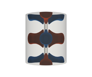
Different from the Taylor–Couette problem (Kumar Reference Kumar2022) in which the 3-D mode exists only when the radius ratio $\eta$ is very small, we observe that the 3-D critical mode always exists in the supergravitational convection. To illustrate this, we plot the bifurcation diagram of critical modes of the 3-D problem in figure 3. For $r_i=0.1$, two 3-D critical modes can be found in the range $Ra\in [9.5\times 10^3,1.8\times 10^4]\cup [3.2\times 10^4,6\times 10^4]$. Otherwise, there is only a single 3-D critical mode of $n=2$, $k\approx 2$, indicating that there is a large-scale 3-D flow structure, which is absent in the classical Rayleigh–Bénard problem and Taylor–Couette problem. To illustrate this 3-D mode of $n=2$, $k\approx 2$, we plot it in figure 4 by setting $Ra=10^8$. The perturbation velocity and thermal fields are shown, indicating that the 3-D mode occupies the whole domain, i.e. it is a large-scale structure. For the other 2-D modes, i.e. the annular mode and the axisymmetric mode, we observe that some of them are nested in the boundary layers, and others are close to the boundary layers but occupy a large region of the domain. This indicates that the 2-D modes that are confined with the boundary layers are actually small-scale structures. This observation may indicate that the small-scale motions in turbulent flows are due to the local instability of boundary layers, while large-scale motion is insensitive to the boundary thickness, which is due to the global instability of the background field.

Figure 3. The wavenumbers of critical modes for (a,b) $r_i=0.1$ and (c,d) $r_i=1$. Dashed lines of the same colour in (b,d) correspond to the 3-D mode.

Figure 4. The critical modes of the Euler–Lagrange equations for $r_i=0.1$, $Ra=10^8$: (a) the 3-D mode with axial length rescaled to $2{\rm \pi}$; (b,c) the radial velocity components of the critical modes.

For $r_i=1$, the bifurcation diagram is more complicated. There are two critical 3-D modes, and the mode of $n=5$ appears and disappears as $Ra$ increases (see the bifurcation diagram in figure 3). It is also interesting that the 2-D axisymmetric mode $q=2$ emerges at approximately $Ra=3\times 10^5$ but disappears forever at approximately $Ra=4.6\times 10^5$. The disappearance and reappearance of these modes causes a ‘discontinuous profile’ of the wavenumbers in figure 3. This is very different from the traditional Rayleigh–Bénard problem: the critical modes never disappear (Plasting & Kerswell Reference Plasting and Kerswell2003; Ding & Kerswell Reference Ding and Kerswell2020), and the corresponding wavenumbers are continuously changing with $Ra$. For the 3-D mode or annular mode, the rising of a new mode can suppress the old mode by changing the profile of the background field (e.g. Plasting & Kerswell Reference Plasting and Kerswell2005). Hence this indicates that in the present problem, the second annular mode is suppressed by the new third mode.

Note that the bifurcation diagram for the 2-D axisymmetric problem is very different from the axisymmetric mode in the 3-D problem (compare figures 3 and 5). The first mode in the 2-D problem is a large-scale structure as the optimal wavenumber remains $O(1)$ as $Ra$ increases. (The bifurcation diagrams for the 2-D axisymmetric problem of $r_i=0.1,1$ are very similar to figure 5. Hence we show only the case $r_i=9$.) But the first axisymmetric mode in the 3-D problem becomes a small-scale structure as $Ra$ increases (its wavenumber scales as $Ra^{1/2}$). This indicates that the first critical mode in the 2-D problem is due to the global instability of the background field, while the first axisymmetric mode in the 3-D problem is due to the instability of the boundary layer. As argued above, that a small-scale structure arises from the instability of boundary layers, it is natural that the ensuing critical modes are of size similar to the boundary layer, i.e. the convective cell height is of the same order as the boundary layer thickness. Typically, the convective cells are nearly square, i.e. $2{\rm \pi} /n\sim \delta$ and $2{\rm \pi} /k_q\sim \delta$ (where $\delta$ is the thickness of either the inner boundary layer or the outer boundary layer). It is clear that the small-scale axisymmetric modes and annular modes in the 3-D problem, as well as the critical modes in the 2-D axisymmetric problem, share common features: $n\sim Ra^{1/2}$, $k_q\sim {Ra^{1/2}}$, which agree well with the analytical suboptimal result that the boundary layer thickness reduces as $\delta \sim Ra^{-1/2}$.

Figure 5. The bifurcation diagram of the critical wavenumber of a 2-D axisymmetric problem for $r_i=9$.

The optimal background fields $\tau$ at $Ra=10^7$ for $r_i=0.1,1,9$ are illustrated in figure 6. When $r_i=0.1$, there is a small discrepancy in the background profiles between the 2-D axisymmetric problem and the full 3-D problem. This discrepancy becomes negligible when $r_i$ increases to $r_i=1$, indicating that the upper bounds yielded from the 2-D and 3-D problems will be very close when the radii ratio is large. In fact, this small discrepancy will also reduce as $Ra$ increases. The present study suggests that 2-D computation gives a good approximation to the optimal bound in supergravitational thermal convection. Moreover, we observe that the bulk temperature of the background field is in excellent agreement with the asymptotic solution $\tau _b=1/(1+\sqrt {\eta })+O(Ra^{-1/2})$. This observation implies that an ‘analytical’ upper bound can be derived from a simple one-dimensional perturbation problem, and imposing the continuity equation as a constraint only improves the prefactor of the bound, which does not change the geometrical dependence or the exponent.

Figure 6. The background temperature profiles for the three typical cases at $Ra=10^7$. Solid lines are for background profiles computed from the 2-D axisymmetric problem, and solid dots are for the corresponding full 3-D problem. The green dashed lines are for $\tau _b=1/(1+\sqrt {\eta })$.

4.3. Comparison with DNS data

We have computed the upper bound of heat transport in supergravitational thermal convection by enforcing partial information of the Navier–Stokes equations. It would be interesting to examine if the maximum heat transfer among solutions of the full Navier–Stokes equations follows the geometrical dependence, and the temperature in the bulk region is close to $1/(1+\sqrt {\eta })$ or $1/(1+\eta )$. Figure 7 illustrates the dependence of the Nusselt number obtained from DNS on the Rayleigh number. The DNS data suggest that the heat transfer in supergravitational thermal convection is reduced by the curvature effect, which is in line with our upper bound analysis. It is also interesting that using our analytical geometrical dependence $\chi (\eta )$, those data from DNS at relatively low $Ra\sim 10^6$ can be brought closer. A close look at the rescaled data suggests that this is not caused by the logarithmic scale of the plot. For example, the rescaled Nusselt number ($Nu/\chi (\eta )$) for $\eta =0.3$ is a little higher than that for $\eta =0.5$ at $Ra=10^6$ or $Ra=2.2\times 10^6$. However, for $Ra>10^7$, the DNS data cannot be well clustered by the geometrical dependence $\chi (\eta )$, and the data gap is even enlarged by the geometrical dependence $\chi (\eta )$ (rescaling using $\chi _a(\eta )$ is worse). Perhaps there are multiple turbulent states in supergravitational convection, e.g. convection with different periods in the azimuthal direction. It is yet unknown which flow state can transfer the most heat, and it is not known whether heat transfer by this flow state follows the geometrical dependence or not. Another more physically plausible reason is that the geometrical dependence is derived from the Euler–Lagrange equations rather than the Navier–Stokes equations, which does not reflect the actual scaling, and correction to the geometrical dependence using more physical information should be made.

Figure 7. The Nusselt number $Nu$ versus the Rayleigh number from DNS; data courtesy of Professor C. Sun. The Prandtl number is $Pr=1$, and the Rossby number gives $Ro^{-1}=1$.

By arguing the equality of temperature scales in the outer and inner boundary layers, Wang et al. (Reference Wang, Jiang, Liu, Zhu and Sun2022) derived that the mean bulk temperature is

(4.25)\begin{equation} \tau_b=\frac{1}{1+\eta^{4/3}}. \end{equation}

Obviously, this bulk temperature is higher than our optimal background temperature $\tau _b=1/(1+\sqrt {\eta })$ and the suboptimal background temperature $\tau _b=1/(1+\eta )$. This difference stems from the assumption of the ratio of the boundary layer thickness. We note that the DNS data by Wang et al. (Reference Wang, Jiang, Liu, Zhu and Sun2022) suggest that the mean temperature approximately follows (4.25), indicating that (4.25) is a better candidate for the bulk temperature than derivations from the upper bound problem for relatively low $Ra$ flows. It is yet unknown if (4.25) is applicable for very large $Ra$ flows, e.g. the ultimate regime flow. Nevertheless, both Wang et al. (Reference Wang, Jiang, Liu, Zhu and Sun2022) and our present work indicate that the bulk temperature deviates from $\tau _b=1/2$ due to the curvature effect, and the mean temperature is elevated by curvature.

It would be interesting to propose a scaling law for the DNS finding by combining (4.25) and an assumption of boundary layer thickness. Since their DNS data suggest that $Nu$ approximately follows $Ra^{1/3}$ ($Nu\sim Ra^{0.32}$ in Wang et al. Reference Wang, Jiang, Liu, Zhu and Sun2022), it is reminiscent of Malkus's classical scaling in Rayleigh–Bénard convection. The $1/3$ scaling can be derived by arguing that the boundary layer is marginally stable or heat flux is independent of the fluid depth. Here, we use the marginal stability assumption to find the geometrical dependence. Since (4.25) well predicts the bulk temperature, the equality of temperature scales in the boundary layers is also reasonable. Thus the assumption of boundary layer thickness ratio $\delta _o/\delta _i=\eta ^{1/3}$ is adopted here too. Moreover, we define inner and outer Rayleigh numbers:

(4.26a,b)\begin{equation} Ra_i=\frac{\alpha \omega^2R_i\delta_i^3\,\Delta T_i}{\nu\kappa},\quad Ra_o=\frac{\alpha \omega^2R_o\delta_o^3\,\Delta T_o}{\nu\kappa}, \end{equation}

where $\Delta T_i=\Delta T/(1+\eta ^{4/3})$, and $\Delta T_o=\eta ^{4/3}\,\Delta T/(1+\eta ^{4/3})$. Hence we have $Ra_o=\eta ^{4/3}\,Ra_i$ and $Ra_o< Ra_i$. Therefore, we argue that the inner boundary layer is marginally stable, while the outer boundary layer is over stable. Consequently, we can assume that the inner Rayleigh number is constant:

(4.27)\begin{equation} Ra_i=\frac{\alpha \omega^2R_i\delta_i^3\,\Delta T_i}{\nu\kappa}=\textrm{const.} \end{equation}

By invoking the definitions of the Rayleigh number $Ra=\frac {1}{2}\alpha \omega ^2(R_i+R_o)\,\Delta T\,d^3/\nu \kappa$ and Nusselt number $Nu=-\ln (\eta )\,\tau _bR_i/\delta _i$, and substituting them into (4.27), we obtain

(4.28a,b)\begin{equation} Nu\sim \chi^*(\eta)\,Ra^{1/3},\quad \chi^*(\eta)={-}\frac{\eta^{4/3}\ln(\eta)}{(1-\eta)(1+\eta)^{1/3}(1+\eta^{4/3})^{4/3}}. \end{equation}

Figure 8 demonstrates that the data rescaled by $\chi ^*(\eta )$ are more compact at high $Ra$ ($Ra>10^7$), and it seems that all rescaled data are converging to a single curve. This indicates that $\chi ^*$ is a good candidate for the geometrical dependence of the Nusselt number in actual supergravitational turbulence when the marginal stability assumption is reliable.

Figure 8. The rescaled Nusselt number $Nu$ versus the Rayleigh number using (4.28a,b). The data are the same as in figure 7.

5. Discussion and conclusion

This study explores the upper bound on supergravitational turbulent convection using Doering–Constantin–Hopf formalism. The take-home message is that heat transport in this system cannot exceed the so-called $1/2$ scaling, and the curvature effect retards heat transport. Our study indicates that different choices of the piecewise background field can yield different geometrical dependence (see the results in § 3 and Appendix B). An interesting finding similar to that of Kumar (Reference Kumar2022) is that the asymptotic solution of the one-dimensional Euler–Lagrange system can yield the correct geometrical dependence for an optimal upper bound. This also implies that enforcing the incompressibility of the perturbations only improves the prefactor.

By rescaling the DNS data from Wang et al. (Reference Wang, Jiang, Liu, Zhu and Sun2022) using our geometrical dependence (4.16a,b), we find that the data can be clustered more compactly when the Rayleigh number $Ra$ is low ($Ra\sim 10^6$). However, at high $Ra$, DNS data do not follow our geometrical dependence. To propose a better geometrical dependence, we applied the marginal stability assumption to discover the geometrical dependence. Interestingly, the geometrical dependence derived from the marginal stability assumption can cluster the DNS data very well (see figure 8). However, Jiang et al. (Reference Jiang, Wang, Liu and Sun2022) reported transition to the ultimate regime in supergravitational convection at higher $Ra$ (${>}10^{10}$) for $\eta =0.5$, and they proposed $Nu\sim Ra^{0.4}$ in the high Rayleigh number regime. This may signify the breakdown of the marginal stability assumption. But it remains unknown how the Nusselt number depends on the geometry in the ultimate regime. Does it depend on our derived geometrical dependence $\chi (\eta )$ from the upper bound problem or the geometrical dependence derived under the marginal stability assumption? This clearly deserves further study in future.

Another interesting finding of our present study indicates that although 3-D large-scale critical modes are crucial for deriving the optimal upper bound, a 2-D axisymmetric problem can yield an asymptotically identical bound as in the full 3-D problem as $Ra\rightarrow \infty$. It indicates that we only need to solve a 2-D Euler–Lagrange system to approximate the optimal upper bound. However, if one considers a 2-D problem with stress-free conditions in future, the bound may be lowered (improved) by imposing further constraints, e.g. a vorticity equation constraint. It has been well known that the best upper bound on 2-D traditional Rayleigh–Bénard convection can be lowered (improved) to $Nu\sim Ra^{5/12}$ (Whitehead & Doering Reference Whitehead and Doering2011; Wen et al. Reference Wen, Chini, Kerswell and Doering2015; Ding & Wen Reference Ding and Wen2020) when stress-free boundary conditions are considered. Thus this raises an interesting question for future study: if one can prove the $5/12$ scaling with geometrical dependence in supergravitational convection between two stress-free boundaries, does that imply that the so-called ultimate regime does not exist, at least in 2-D axisymmetric flow? However, for a 3-D flow, there is no room to improve the $1/2$ scaling derived in the present study in the framework of Doering–Constantin–Hopf formalism (Ding & Kerswell Reference Ding and Kerswell2020).

Funding

I was supported by NSFC (no. 52176065) and Fundamental Research Funds for the Central Universities (AUGA9803100122, AUGA9803504221, 2022FRFK060022). I thank Professor C. Sun from Tsinghua University for sharing the original data and pointing out several typos in an early version. I also thank Dr B. Wen for checking the analytical suboptimal results, and the reviewers for their many important suggestions, which significantly improved the present work. In particular, I appreciate the second reviewer for the many constructive suggestions and careful reading of this work, which helped me to minimize many typos.

Declaration of interests

The author reports no conflict of interest.

Appendix A. The particular solution for $\inf \mathscr {G}$

To find the minimum of $\mathscr {G}$, we construct the Lagrangian

(A1)\begin{equation} {L}=\left\langle a\,|\boldsymbol{\nabla}\boldsymbol{u}|^2+|\boldsymbol{\nabla}\theta|^2+2\,\sqrt{Ra}\,\theta u\,\frac{\textrm{d}\tau}{\textrm{d}r}+{2a\,\frac{1-\eta}{1+\eta}\,r\,\frac{\partial\theta}{\partial r}}\right\rangle-\langle p\,\boldsymbol{\nabla}\boldsymbol{\cdot}\boldsymbol{u}\rangle. \end{equation}

Variation of $L$ gives the equations

(A2)$$\begin{gather} \delta{L}/\delta\boldsymbol{u}:={-}2a\,\nabla^2\boldsymbol{u}+2\,\sqrt{Ra}\,\theta\,\frac{\textrm{d}\tau}{\textrm{d}r}\,\boldsymbol{e}_r+\boldsymbol{\nabla} p=0, \end{gather}$$
(A3)$$\begin{gather}\delta{L}/\delta p:=\boldsymbol{\nabla}\boldsymbol{\cdot} \boldsymbol{u}=0, \end{gather}$$
(A4)$$\begin{gather}\delta{L}/\delta\theta:={-}2\,\nabla^2\theta+2\,\sqrt{Ra}\,u\,\frac{\textrm{d}\tau}{\textrm{d}r}-4a\,\frac{1-\eta}{1+\eta}=0. \end{gather}$$

Hence it is easy to show that $(\boldsymbol {u},\theta )=(0,\theta (r))$ is a particular solution, and we obtain

(A5)\begin{equation} \left.\begin{gathered} \boldsymbol{u}=0,\quad \theta(r)={-}\frac{a}{2}\,\frac{1-\eta}{1+\eta}\,(r^2-r_i^2)-\frac{a}{2\ln(\eta)}\ln(r/r_i),\\ {p=p_i-2\,\sqrt{Ra}\int^r_{r_i}{\theta}(r')\,\frac{\textrm{d}\tau(r')}{\textrm{d}r'}\,\textrm{d}r'}, \end{gathered}\right\} \end{equation}

where $p_i$ is a constant. This particular solution can be used to remove the linear terms in $\mathscr {G}$.

Appendix B. Different background fields can yield different geometrical dependence

Inspired by the asymptotic solution (4.15) and the numerical result $a=1/3$, we revisit the analysis in § 3 by choosing the following background profile (setting $c=1/(1+\sqrt {\eta })$ in (3.1)):

(B1) \begin{equation} \tau=\left\{\!\!\begin{array}{@{}ll@{}} \displaystyle\dfrac{1}{1+\sqrt{\eta}}\,\dfrac{1}{\ln((r_i+\delta_i)/r_i)}\ln(r/r_i), & z\in[r_i,r_i+\delta_i],\\ \displaystyle\dfrac{1}{1+\sqrt{\eta}}, & z\in(r_i+\delta_i,r_o-\delta_o],\\ \displaystyle 1-\dfrac{\sqrt{\eta}}{1+\sqrt{\eta}}\,\dfrac{1}{\ln((r_o-\delta_o)/r_o)}\ln(r/r_o), & z\in(r_o-\delta_o,r_o]. \end{array} \right. \end{equation}

Moreover, we also impose the heat flux conservative condition across the two cylinders:

(B2)\begin{equation} \frac{1}{\ln((r_i+\delta_i)/r_i)}={-}\frac{\sqrt{\eta}}{\ln((r_o-\delta_o)/r_o)}. \end{equation}

As $Ra\rightarrow \infty$, $\delta _i\ll r_i$ and $\delta _o\ll r_o$, (B2) simplifies to $\delta _i=\sqrt {\eta }\,\delta _o$.

Using the new background profile (B1), and following exactly the same inequality analysis as in §3, we can obtain

(B3)\begin{equation} \mathcal{C}=\frac{1}{1+\sqrt{\eta}}\,\delta_i+\frac{\sqrt{\eta}}{1+\sqrt{\eta}}\,\delta_o=\frac{2}{1+\sqrt{\eta}}\,\delta_i\quad \textrm{as}\ Ra\rightarrow\infty. \end{equation}

Using (3.15a,b) and (B3), we have

(B4)\begin{equation} \frac{2}{1+\sqrt{\eta}}\,\delta_i=\frac{1}{\sqrt{3\,Ra}}\ \Rightarrow\ \delta_i=\frac{1+\sqrt{\eta}}{2\sqrt{3}}\,Ra^{{-}1/2},\quad Ra\rightarrow\infty. \end{equation}

Using (3.18) and the new background profile (B1), we obtain

(B5)\begin{align} Nu\lesssim -\frac{3}{2}\,\frac{\eta\ln(\eta)}{(1-\eta)(1+\sqrt{\eta})^2}\left(\frac{1}{\delta_i}+\frac{1}{\delta_o}\right)={-}\frac{3\sqrt{3}\eta\ln(\eta)}{(1-\eta)(1+\sqrt{\eta})^2}\,Ra^{1/2},\quad Ra\rightarrow\infty. \end{align}

Note that the above analysis yields the same geometrical dependence as (4.16a,b) but with a higher coefficient $3\sqrt {3}$ (compared with $3/2$). This is the direct evidence that different background profiles can yield different geometrical dependence. However, (3.23) is slightly better (smaller) than (B5) for all $\eta \in (0,1)$, although it does not yield the correct analytical geometrical dependence.

Appendix C. The Lagrangian in terms of Fourier modes

Using the expansion in (4.19)–(4.21), the Lagrangian $\mathscr {L}$ is expressed as

(C1) \begin{align} \mathscr{L}&=nu-\frac{a}{4}\sum_{n=1}^N\int_{r_i}^{r_o}r\left[\left(\left(\frac{\textrm{ d}u_n}{\textrm{d}r}\right)^2+\left(\frac{\textrm{d}v_n}{\textrm{ d}r}\right)^2+\left(\frac{\textrm{d}w_n}{\textrm{ d}r}\right)^2\right)\right.\nonumber\\ &\quad \left.{}\vphantom{\left(\frac{\textrm{ d}u_n}{\textrm{d}r}\right)^2}+\frac{(nu_n+v_n)^2+(u_n+nv_n)^2}{r^2}\right]\textrm{ d}r\nonumber\\ &\quad -\frac{a}{4}\sum_{n=1}^N\int_{r_i}^{r_o}rk_n^2(u_n^2+v_n^2+w_n^2)\,\textrm{ d}r-\frac{1}{4}\sum_{n=1}^N\int_{r_i}^{r_o}r\left(\left(\frac{\textrm{ d}\theta_n}{\textrm{ d}r}\right)^2+\frac{n^2\theta^2_n}{r^2}+k_n^2\theta_n^2\right)\textrm{ d}r\nonumber\\ &\quad-\frac{1}{4}\sum_{n=1}^N\int_{r_i}^{r_o}2\,\sqrt{Ra}\,ru_n\theta_n\,\frac{\textrm{d}\tau}{\textrm{ d}r}\,\textrm{ d}r+\frac{1}{4}\int_{r_i}^{r_o}rp_n\left(\frac{\textrm{ d}u_n}{\textrm{ d}r}+\frac{u_n}{r}+\frac{nv_n}{r}+k_nw_n\right)\textrm{ d}r\nonumber\\ &\quad -\frac{a}{2}\sum_{m=1}^{M}\int_{r_i}^{r_o}r\left[\left(\left(\frac{\textrm{d}u_m}{\textrm{d}r}\right)^2+\left(\frac{\textrm{d}v_m}{\textrm{d}r}\right)^2+\left(\frac{\textrm{d}w_m}{\textrm{d}r}\right)^2\right)\right.\nonumber\\ &\quad \left.{}\vphantom{\left(\frac{\textrm{d}u_n}{\textrm{d}r}\right)^2}+\frac{(mu_m+v_m)^2+(u_m+mv_m)^2}{r^2}\right]\textrm{d}r\nonumber\\ &\quad -\frac{1}{2}\sum_{m=1}^M\int_{r_i}^{r_o}r\left(\left(\frac{\textrm{d}\theta_m}{\textrm{d}r}\right)^2+\frac{m^2\theta^2_m}{r^2}\right)\textrm{d}r-\frac{1}{2}\sum_{m=1}^M\int_{r_i}^{r_o}2\,\sqrt{Ra}\,ru_m\theta_m\,\frac{\textrm{d}\tau}{\textrm{d}r}\,\textrm{d}r\nonumber\\ &\quad +\frac{1}{2}\sum_{m=1}^M\int_{r_i}^{r_o}rp_m\left(\frac{\textrm{ d}u_m}{\textrm{d}r}+\frac{u_m}{r}+\frac{mv_m}{r}\right)\textrm{ d}r\nonumber\\ &\quad -\frac{a}{2}\sum_{q=1}^{Q}\int_{r_i}^{r_o}r\left[\left(\left(\frac{\textrm{ d}u_q}{\textrm{d}r}\right)^2+\left(\frac{\textrm{d}v_q}{\textrm{ d}r}\right)^2+\left(\frac{\textrm{d}w_q}{\textrm{ d}r}\right)^2\right)\right.\nonumber\\ &\quad \left.{}+\frac{u_q^2}{r^2}+\frac{v_q^2}{r^2}+k_q^2(u_q^2+v_q^2+w_q^2)\right]\textrm{ d}r\nonumber\\ &\quad -\frac{1}{2}\sum_{q=1}^Q\int_{r_i}^{r_o}r\left(\left(\frac{\textrm{ d}\theta_q}{\textrm{d}r}\right)^2+k_q^2\theta^2_q\right)\textrm{ d}r-\frac{1}{2}\sum_{m=1}^M\int_{r_i}^{r_o}2\,\sqrt{Ra}\,ru_m\theta_m\frac{\textrm{ d}\tau}{\textrm{d}r}\textrm{d}r\nonumber\\ &\quad +\frac{1}{2}\sum_{q=1}^Q\int_{r_i}^{r_o}rp_q\left(\frac{\textrm{ d}u_q}{\textrm{d}r}+\frac{u_q}{r}+k_qw_q\right)\textrm{d}r. \end{align}

Variational of $\mathscr {L}$ with respect to $k_n$ and $k_q$ gives the optimal conditions for wavenumbers.

References

Ahlers, G., Grossmann, S. & Lohse, D. 2009 Heat transfer and large scale dynamics in turbulent Rayleigh–Bénard convection. Rev. Mod. Phys. 81, 503537.CrossRefGoogle Scholar
Bouillaut, V., Lepot, S., Aumaître, S. & Gallet, B. 2019 Transition to the ultimate regime in a radiatively driven convection experiment. J. Fluid Mech. 861, R5.CrossRefGoogle Scholar
Busse, F. 1969 On Howard's upper bound for heat transport by turbulent convection. J. Fluid Mech. 37, 457477.CrossRefGoogle Scholar
Chernyshenko, S. 2022 Relationship between the methods of bounding time averages. Phil. Trans. R. Soc. Lond. A 380, 20210044.Google ScholarPubMed
Chernyshenko, S., Goulart, P., Huang, D. & Papachristodoulou, A. 2014 Polynomial sum of squares in fluid dynamics: a review with a look ahead. Phil. Trans. R. Soc. Lond. B 372, 20130350.Google ScholarPubMed
Choffrut, A., Nobili, C. & Otto, F. 2016 Upper bounds on Nusselt number at finite Prandtl number. J. Differ. Equ. 260, 38603880.CrossRefGoogle Scholar
Ding, Z. & Kerswell, R.R. 2020 Exhausting the background approach for bounding the heat transport in Rayleigh–Bénard convection. J. Fluid Mech. 889, A33.CrossRefGoogle Scholar
Ding, Z. & Wen, B. 2020 A note on upper bound for heat transport in two-dimensional Rayleigh–Bénard convection. Intl Commun. Heat Mass Transfer 117, 104785.CrossRefGoogle Scholar
Doering, C. & Constantin, P. 1996 Variational bounds on energy dissipation in incompressible flows. III. Convection. Phys. Rev. E 53, 5957.CrossRefGoogle ScholarPubMed
Ecke, R.E. & Shishkina, O. 2023 Turbulent rotating Rayleigh–Bénard convection. Annu. Rev. Fluid Mech. 55, 603638.CrossRefGoogle Scholar
Fantuzzi, G., Arslan, A. & Wynn, A. 2022 The background method: theory and computations. Phil. Trans. R. Soc. Lond. A 380, 20210038.Google ScholarPubMed
He, X., Funfschilling, D., Nobach, H., Bodenschatz, E. & Ahlers, G. 2012 Transition to the ultimate state of turbulent Rayleigh–Bénard convection. Phys. Rev. Lett. 108, 024502.CrossRefGoogle Scholar
Howard, L. 1963 Heat transport by turbulent convection. J. Fluid Mech. 17, 405.CrossRefGoogle Scholar
Ierley, G.R., Plasting, S. & Kerswell, R.R. 2006 Infinite-Prandtl-number convection. Part 2. A singular limit of upper bound theory. J. Fluid Mech. 560, 159227.CrossRefGoogle Scholar
Iyer, K.P., Scheel, J.D., Schumacher, J. & Sreenivasan, K.R. 2020 Classical $1/3$ scaling of convection holds up to $Ra=10^{15}$. Proc. Natl Acad. Sci. USA 117, 75947598.CrossRefGoogle ScholarPubMed
Jiang, H., Wang, D., Liu, S. & Sun, C. 2022 Experimental evidence for the existence of the ultimate regime in rapidly rotating turbulent thermal convection. Phys. Rev. Lett. 129, 204502.CrossRefGoogle ScholarPubMed
Jiang, H., Zhu, X., Wang, D., Huisman, S. & Sun, C. 2020 Supergravitational turbulent thermal convection. Sci. Adv. 6, eabb8676.CrossRefGoogle ScholarPubMed
Kraichnan, R.H. 1962 Turbulent thermal convection at arbitrary Prandtl number. Phys. Fluids 5, 13741389.CrossRefGoogle Scholar
Kumar, A. 2022 Geometrical dependence of optimal bounds in Taylor–Couette flow. J. Fluid Mech. 948, A11.CrossRefGoogle Scholar
Lindborg, E. 2023 Scaling in Rayleigh–Bénard convection. J. Fluid Mech. 956, A34.CrossRefGoogle Scholar
Lohse, D. & Xia, K.Q. 2010 Small-scale properties of turbulent Rayleigh–Bénard convection. Annu. Rev. Fluid Mech. 42, 335364.CrossRefGoogle Scholar
Malkus, M. 1954 The heat transport and spectrum of thermal turbulence. Proc. R. Soc. Lond. A 225, 196.Google Scholar
Otto, F. & Seis, C. 2011 Rayleigh–Bénard convection: improved bounds on the Nusselt number. J. Math. Phys. 52, 083702.CrossRefGoogle Scholar
Plasting, S. & Ierley, G.R. 2005 Estimates of heat transport in infinite Prandtl number convection. Part 1. Conservative bounds. J. Fluid Mech. 542, 343363.CrossRefGoogle Scholar
Plasting, S. & Kerswell, R.R. 2003 Improved upper bound on the energy dissipation rate in plane Couette flow: the full solution to Busse's problem and the Constantin–Doering–Hopf problem with one-dimensional background field. J. Fluid Mech. 477, 363379.CrossRefGoogle Scholar
Plasting, S. & Kerswell, R.R. 2005 A friction factor bound for transitional pipe flow. Phys. Fluids 17, 011706.CrossRefGoogle Scholar
Rosa, R. & Temam, R. 2022 Optimal minimax bounds for time and ensemble averages for the incompressible Navier–Stokes equations. Pure Appl. Funct. Anal. 7 (1), 327355.Google Scholar
Seis, C. 2015 Scaling bounds on dissipation in turbulent flows. J. Fluid Mech. 777, 591603.CrossRefGoogle Scholar
Urban, P., Musilová, V. & Skrbek, L. 2011 Efficiency of heat transfer in turbulent Rayleigh–Bénard convection. Phys. Rev. Lett. 107, 014302.CrossRefGoogle ScholarPubMed
Wang, D., Jiang, H., Liu, S., Zhu, X. & Sun, C. 2022 Effects of radius ratio on annular centrifugal Rayleigh–Bénard convection. J. Fluid Mech. 930, A19.CrossRefGoogle Scholar
Wen, B., Chini, G., Kerswell, R. & Doering, C. 2015 Time-stepping approach for solving upper-bound problems: application to two-dimensional Rayleigh–Bénard convection. Phys. Rev. E 92, 043012.CrossRefGoogle ScholarPubMed
Whitehead, J. & Doering, C. 2011 Ultimate state of two-dimensional Rayleigh–Bénard convection between free-slip fixed-temperature boundaries. Phys. Rev. Lett. 106, 244501.CrossRefGoogle ScholarPubMed
Zhong, J., Wang, D. & Sun, C. 2023 From sheared annular centrifugal Rayleigh–Bénard convection to radially heated Taylor–Couette flow: exploring the impact of buoyancy and shear on heat transfer and flow structure. J. Fluid Mech. 972, A29.CrossRefGoogle Scholar
Zhu, X., Mathai, V., Stevens, R.J.A.M., Verzicco, R. & Lohse, D. 2018 Transition to the ultimate regime in two-dimensional Rayleigh–Bénard convection. Phys. Rev. Lett. 120, 144502.CrossRefGoogle Scholar
Figure 0

Figure 1. The balance parameter versus the Rayleigh number. Solid lines are computed by solving the full 3-D Euler–Lagrange equations, and dashed lines are computed from the 2-D axisymmetric problem. The green line is derived from the analytical suboptimal problem: $a=1/3$.

Figure 1

Figure 2. The Nusselt number $Nu$ versus the Rayleigh number. Solid lines are computed by solving the full 3-D Euler–Lagrange equations, and dashed lines are computed from the 2-D axisymmetric problem.

Figure 2

Figure 3. The wavenumbers of critical modes for (a,b) $r_i=0.1$ and (c,d) $r_i=1$. Dashed lines of the same colour in (b,d) correspond to the 3-D mode.

Figure 3

Figure 4. The critical modes of the Euler–Lagrange equations for $r_i=0.1$, $Ra=10^8$: (a) the 3-D mode with axial length rescaled to $2{\rm \pi}$; (b,c) the radial velocity components of the critical modes.

Figure 4

Figure 5. The bifurcation diagram of the critical wavenumber of a 2-D axisymmetric problem for $r_i=9$.

Figure 5

Figure 6. The background temperature profiles for the three typical cases at $Ra=10^7$. Solid lines are for background profiles computed from the 2-D axisymmetric problem, and solid dots are for the corresponding full 3-D problem. The green dashed lines are for $\tau _b=1/(1+\sqrt {\eta })$.

Figure 6

Figure 7. The Nusselt number $Nu$ versus the Rayleigh number from DNS; data courtesy of Professor C. Sun. The Prandtl number is $Pr=1$, and the Rossby number gives $Ro^{-1}=1$.

Figure 7

Figure 8. The rescaled Nusselt number $Nu$ versus the Rayleigh number using (4.28a,b). The data are the same as in figure 7.