Three-dimensional soft streaming

Abstract

Viscous streaming is an efficient rectification mechanism to exploit flow inertia at small scales for fluid and particle manipulation. It typically entails a fluid vibrating around an immersed solid feature that, by concentrating stresses, modulates the emergence of steady flows of useful topology. Motivated by its relevance in biological and artificial settings characterized by soft materials, recent studies have theoretically elucidated, in two dimensions, the impact of body elasticity on streaming flows. Here, we generalize those findings to three dimensions, via the minimal case of an immersed soft sphere. We first improve existing solutions for the rigid-sphere limit, by considering previously unaccounted terms. We then enable body compliance, exposing a three-dimensional, elastic streaming process available even in Stokes flows. Such effect, consistent with two-dimensional analyses but analytically distinct, is validated against direct numerical simulations and shown to translate to bodies of complex geometry and topology, paving the way for advanced forms of flow control.

1. Introduction

This study investigates the effects of body elasticity on three-dimensional viscous streaming. Viscous streaming, an inertial phenomenon, refers to the steady, rectified flows that emerge when a fluid oscillates around a localized microfeature. Given its ability to remodel surrounding flows over short time and length scales, streaming has found application in multiple aspects of microfluidics, from particle manipulation (Lutz, Chen & Schwartz 2003, 2005; Marmottant & Hilgenfeldt 2004; Lutz, Chen & Schwartz 2006; Wang, Jalikop & Hilgenfeldt 2011; Chong et al. 2013; Chen & Lee 2014; Klotsa et al. 2015; Thameem, Rallabandi & Hilgenfeldt 2017) and chemical mixing (Liu et al. 2002; Lutz et al. 2003, 2005; Ahmed et al. 2009) to vesicle transport and lysis (Marmottant & Hilgenfeldt 2003, 2004). Recently, the use of multi-curvature streaming bodies has expanded the ability to manipulate flows, leading to compact, robust and tunable devices for filtering and separating both synthetic and biological particles (Parthasarathy, Chan & Gazzola 2019; Bhosale, Parthasarathy & Gazzola 2020; Chan et al. 2022; Bhosale et al. 2022b). More recently yet, motivated by medical and biological applications and building upon past theoretical studies (Wang 1965; Riley 1966, 1998, 2001; Rednikov et al. 2006; Rednikov & Sadhal 2011; Sadhal 2012; Sadhal, Laurell & Lenshof 2014), the effect of body compliance has been considered (Anand & Christov 2020), with one of the studies yielding a first two-dimensional streaming theory for soft cylinders (Bhosale, Parthasarathy & Gazzola 2022a). Its major outcome is encapsulated in the relation

(1.1)\begin{equation} \langle \psi_1 \rangle = \sin 2 \theta \left[ \varTheta(r) + \varLambda(r) \right], \end{equation}

where $\langle \psi _1 \rangle$ is the time-averaged Stokes streamfunction and $r$ and $\theta$ are the radial and polar coordinates in the cylindrical system. This relation reveals an additional streaming process $\varLambda (r)$, purely induced by body elasticity, that is available even in Stokes flows where rigid-body streaming $\varTheta (r)$ cannot exist (Holtsmark et al. 1954). Elasticity modulation has then been shown to achieve streaming configurations similar to those of rigid bodies, but at significantly lower frequencies. This frequency reduction has relevant implications, as it renders viscous streaming accessible within the limits of biological actuation.

In this work, we extend this understanding to three dimensions by examining the minimal case of an oscillating, soft sphere. We first present an improved theoretical solution for the rigid-sphere case by augmenting the derivation of Lane (1955) with a previously unaccounted term related to vortex stretching. Our formulation is shown to significantly enhance quantitative agreement with direct numerical simulations and experiments. Next, within the same theoretical framework, we consider body elasticity and seek a modified streaming solution dependent on material compliance. We recover an independent elastic modification term, similar in nature to the above two-dimensional result but analytically distinct. We then demonstrate the accuracy of our theory against direct numerical simulations, and show how observed elasticity effects may translate to bodies of complex geometry and topology, further expanding the potential utility of soft streaming.

2. Problem set-up and governing equations

We derive the streaming solution by considering the set-up shown in figure 1, where a three-dimensional viscoelastic solid sphere $\varOmega _e$ of radius $a$ is immersed in a viscous fluid $\varOmega _f$. The fluid oscillates with velocity $V(t) = \epsilon a \omega \cos \omega t$, where $\epsilon$, $\omega$ and $t$ represent the non-dimensional amplitude, angular frequency and time. Following our previous set-up for a soft two-dimensional cylinder (Bhosale et al. 2022a), we kinematically enforce zero strain and velocity near the sphere's centre by ‘pinning’ the sphere with a rigid inclusion $\varGamma$ of radius $b < a$, the boundary of which is denoted by $\partial \varGamma$. We choose to ‘pin’ the sphere to suppress its rigid-body motion and simplify mathematical treatment. Experimentally, this approach may be realized by coating with a soft material a rigid sphere, which in turn can be suspended in flow as in Kotas, Yoda & Rogers (2007) or Lane (1955). Finally, we denote by $\partial \varOmega$ the boundary between the elastic solid and the viscous fluid.

Figure 1. Problem set-up. (a) Three-dimensional viscoelastic solid sphere $\varOmega _e$ of radius $a$ with a rigid inclusion (pinned zone $\varGamma$ of radius $b$), immersed in viscous fluid $\varOmega _f$. In this study, we deploy a spherical coordinate system where $(r, \theta, \phi )$ are the radial, polar and azimuthal coordinates. The sphere is exposed to an oscillatory flow with far-field velocity $V(t) = \epsilon a \omega \cos (\omega t)$ in the $x$ direction, along the axis of symmetry. (b) Two-dimensional axisymmetric cross-section of the elastic sphere.

Both fluid and solid are assumed to be isotropic and incompressible, where the fluid is Newtonian with kinematic viscosity $\nu _f$ and density $\rho _f$, and the solid follows the Kelvin–Voigt viscoelastic model. Characteristic of soft biological materials (Bower 2009), elastic stresses within the solid are modelled via neo-Hookean hyperelasticity with shear modulus $G$, kinematic viscosity $\nu _e$ and density $\rho _e$. However, we will later show that the choice of hyperelastic or viscoelastic model does not affect the theory. To simplify nomenclature, we henceforth refer to the viscoelastic solid as an elastic solid.

The dynamics in the fluid and solid phases is governed by the incompressible Cauchy momentum equations, non-dimensionalized using the characteristic scales of velocity $V = \epsilon a \omega$, length $L = a$, time $T = 1 / \omega$ and hydrostatic pressure $P = \mu _f V / L = \mu _f \epsilon \omega$ (derivation details are in §§ 1 and 10 of the supplementary material available at https://doi.org/10.1017/jfm.2023.1050):

(2.1) \begin{align} \left. \begin{aligned} \textrm{Incomp.} & \left\{ {\boldsymbol{\nabla}} \boldsymbol{\cdot} {\boldsymbol{v}} = 0, {\boldsymbol{x}}\in \varOmega_f \cup \varOmega_e \right.,\\ \textrm{Fluid} & \left\{ \dfrac{\partial {{\boldsymbol{v}}}}{\partial {t}} + \epsilon ({{\boldsymbol{v}}} \boldsymbol{\cdot} {{\boldsymbol{\nabla}}}) {{\boldsymbol{v}}} = \dfrac{1}{M^2} \big(-{\boldsymbol{\nabla}}{p} + {\nabla^2} {{\boldsymbol{v}}} \big), {{\boldsymbol{x}}}\in\varOmega_f \right.,\\ \textrm{Solid} & \left\{ \alpha \mathrm{Cau} \left( \dfrac{\partial {{\boldsymbol{v}}}}{\partial {t}} + \epsilon ({{\boldsymbol{v}}} \boldsymbol{\cdot} {{\boldsymbol{\nabla}}}) {{\boldsymbol{v}}} \right) = \dfrac{\mathrm{Cau}}{M^2} \big( -{\boldsymbol{\nabla}} {p} + \beta {\nabla^2} {{\boldsymbol{v}}} \big) + {{\boldsymbol{\nabla}}} \boldsymbol{\cdot} ({{\boldsymbol{\mathsf{F}}}} {{\boldsymbol{\mathsf{F}}}}^{\rm T})' ,{{\boldsymbol{x}}}\in\varOmega_e, \right. \end{aligned} \right\} \end{align}

where ${\boldsymbol {v}}$ and $p$ are the velocity and pressure fields and ${\boldsymbol{\mathsf{F}}}$ is the deformation gradient tensor, defined as ${\boldsymbol{\mathsf{F}}} = {\boldsymbol{\mathsf{I}}} + {\boldsymbol {\nabla }} {\boldsymbol {u}}$, where ${\boldsymbol{\mathsf{I}}}$ is the identity, ${\boldsymbol {u}} = {\boldsymbol {x}} - {\boldsymbol {X}}$ is the material displacement field and ${\boldsymbol {x}}$, ${\boldsymbol {X}}$ are the position of a material point after deformation and at rest, respectively. We comment that we uniformly refer to the hydrostatic stress in both the fluid and solid phases as ‘pressure’ ($\kern 0.06em p$) to avoid cluttering the terminology. The prime symbol $'$ on a tensor denotes its deviatoric. The key non-dimensional parameters within this system are the scaled oscillation amplitude $\epsilon$, Womersley number $M = a \sqrt {\rho _f \omega / \mu _f}$, Cauchy number $\mathrm {Cau} = \epsilon \rho _f a^2 \omega ^2 / G$, density ratio $\alpha = \rho _e / \rho _f$ and viscosity ratio $\beta = \mu _e / \mu _f$. Physically, the Womersley number ($M$) represents the ratio of inertial to viscous forces and the Cauchy number ($\mathrm {Cau}$) represents the ratio of inertial to elastic forces. Therefore, a higher $M$ corresponds to stronger dominance of inertia in the fluid environment and higher $\mathrm {Cau}$ values correspond to increasingly soft bodies. We further remark that the inverse of the Womersley number ($1/M$) is equivalent to the non-dimensionalized viscous boundary layer thickness ($\delta _{AC} / a$), and thus captures a length scale critical to microfluidic processes.

We then impose a set of boundary conditions upon the governing equations, consistent with Lane (1955):

(2.2)$$\begin{gather} \textrm{Pinned zone } \left\{{\boldsymbol{u}} = 0, {\boldsymbol{v}} = 0,~{\boldsymbol{x}}\in \varGamma ,\right. \end{gather}$$

(2.3)$$\begin{gather}\textrm{Interface velocity } \left\{ {\boldsymbol{v}}_e = {\boldsymbol{v}}_f,~{\boldsymbol{x}}\in\partial\varOmega \right., \end{gather}$$

(2.4) $$\begin{gather}\textrm{Interface stresses } \begin{cases} {\boldsymbol{\sigma}}_{f} ={-}p{\boldsymbol{\mathsf{I}}} + ({\boldsymbol{\nabla}} {\boldsymbol{v}} + {\boldsymbol{\nabla}} {\boldsymbol{v}}^{\rm T}), {\boldsymbol{x}}\in\varOmega_f ,\\ {\boldsymbol{\sigma}}_{e} ={-}p{\boldsymbol{\mathsf{I}}} + \beta ({\boldsymbol{\nabla}} {\boldsymbol{v}} + {\boldsymbol{\nabla}} {\boldsymbol{v}}^{\rm T}) +\dfrac{M^2}{\mathrm{Cau}}({\boldsymbol{\mathsf{F}}} {\boldsymbol{\mathsf{F}}}^{\rm T})', {\boldsymbol{x}}\in\varOmega_e, \\ {\boldsymbol{n}} \boldsymbol{\cdot} {\boldsymbol{\sigma}}_e \boldsymbol{\cdot} {\boldsymbol{n}} = {\boldsymbol{n}} \boldsymbol{\cdot} {\boldsymbol{\sigma}}_f \boldsymbol{\cdot} {\boldsymbol{n}}, {\boldsymbol{x}}\in\partial\varOmega,\\ {\boldsymbol{n}} \boldsymbol{\cdot} {\boldsymbol{\sigma}}_e \boldsymbol{\cdot} {\boldsymbol{t}} = {\boldsymbol{n}} \boldsymbol{\cdot} {\boldsymbol{\sigma}}_f \boldsymbol{\cdot} {\boldsymbol{t}}, {\boldsymbol{x}}\in\partial\varOmega, \end{cases} \end{gather}$$

(2.5)$$\begin{gather}\textrm{Far field } \left\{{\boldsymbol{v}}(|{\boldsymbol{x}}| \to \infty) = \cos t \hat{i}, {\boldsymbol{x}}\in \varOmega_{f},\right. \end{gather}$$

where (2.2) is the pinned-zone rigidity constraint, (2.3) is the no-slip boundary condition between and solid and fluid phases, (2.4) dictates stress continuity and (2.5) is the far-field flow velocity. We use subscripts $e$ and $f$ to denote elastic and fluid phases, respectively, wherever ambiguity may arise. Next, we identify ranges of relevant parameters and solve (2.1) via perturbation theory.

3. Perturbation series solution

In viscous streaming applications, typically we have small non-dimensional oscillation amplitudes $\epsilon \ll {1}$ (Wang 1965; Bertelsen, Svardal & Tjøtta 1973; Lutz et al. 2005), density ratio $\alpha$ and viscosity ratio $\beta$ of ${O} \left ( 1 \right )$, and Womersley number $M \sim {O} \left ( 1 \right )$ (Marmottant & Hilgenfeldt 2004; Lutz et al. 2006). For the Cauchy number $\mathrm {Cau}$, we apply the same treatment as in Bhosale et al. (2022a), where we use $\mathrm {Cau} = 0$ for a rigid body and $\mathrm {Cau} = \kappa \epsilon$ with $\kappa = {O} \left ( 1 \right )$ for elastic bodies. The latter assumption implies that $\mathrm {Cau} \ll 1$, which physically means that the body is weakly elastic. We make this assumption for two reasons. First, we choose $\mathrm {Cau}$ to be small to simplify the treatment of hyperelastic materials, whose nonlinearities become mathematically challenging for $\mathrm {Cau} \geq {O} \left ( 1 \right )$. Second, matching $\mathrm {Cau}$ with $\epsilon$ simplifies the asymptotic expansion, while preserving the practical generality of the results (for details, see supplementary material § 2 of Bhosale et al. (2022a)).

We then seek a perturbation series solution of (2.1) by asymptotically expanding all relevant fields in powers of $\epsilon$. Our derivation closely follows the approach taken by Bhosale et al. (2022a) for two-dimensional elastic cylinders, while augmenting it to encompass three-dimensional settings. Then, the zeroth-order solution reduces to a rigid sphere in a purely oscillatory flow governed by the unsteady Stokes equation (Lane 1955). The first-order solution is subsequently derived in two stages. First, we obtain the deformation of the elastic body resulting from the flow field at zeroth order. Second, we incorporate the elastic feedback into the streaming solution by using the obtained body deformations as boundary conditions for the flow at ${O} \left ( \epsilon \right )$. The steps are outlined below, with details listed in the supplementary material.

We start by perturbing to ${O} \left ( \epsilon \right )$ all physical quantities $q$, which include ${\boldsymbol {v}}$, ${\boldsymbol {u}}$, $p$, $\varOmega$, ${\boldsymbol {n}}$, ${\boldsymbol {t}}$, as

(3.1)\begin{equation} q \sim q_0 + \epsilon q_1 + \mathcal{O} (\epsilon^2) \end{equation}

and substitute them into the governing equations (2.1) and boundary conditions (2.2)–(2.5). Steps are explicitly reported in the supplementary material (equations (1.17)–(1.26)), where subscripts ($0, 1,\ldots$) refer to the solution order. We remark that the zeroth order $q_0$ of quantities non-dimensionalized by $V=\epsilon a \omega$ corresponds to order ${O} \left ( \epsilon \right )$ in dimensional form. Thus, our expansion remains consistent with previous examples of streaming literature (Longuet-Higgins 1998; Spelman & Lauga 2017) where enumeration starts from the first order (supplementary material, equation (1.17)). Next, we adopt the geometrically convenient spherical coordinate system $(r, \theta, \phi )$, with radial coordinate $r$, polar angle $\theta$, azimuthal angle $\phi$ and origin at the centre of the sphere. The horizontal axis direction ${\boldsymbol {i}}$ corresponds to $\theta = 0$.

3.1. Zeroth-order ${O} \left ( 1 \right )$ solution

The governing equations and boundary conditions in the solid phase at zeroth order ${O} \left ( 1 \right )$ simplify to

(3.2)\begin{equation} {\boldsymbol{\nabla}} \boldsymbol{\cdot} (({\boldsymbol{\mathsf{I}}} + {\boldsymbol{\nabla}} {\boldsymbol{u}}_0) ({\boldsymbol{\mathsf{I}}} + {\boldsymbol{\nabla}} {\boldsymbol{u}}_0)^{\rm T})' = 0, \quad r \leq 1;\ {\boldsymbol{u}}_0|_{r = \zeta} = 0, \end{equation}

where $\zeta = b / a$ is the non-dimensional radius of the pinned zone. Since at this order $\mathrm {Cau} = \kappa \epsilon = 0$, the solution of (3.2) physically corresponds to a fixed, rigid sphere with

(3.3)\begin{equation} \partial\varOmega_0 = r = 1;\quad {\boldsymbol{u}}_0 = 0,\quad {\boldsymbol{v}}_{0} = \frac{\partial {\boldsymbol{u}}_0}{\partial t} = 0 ,\quad r \leq 1. \end{equation}

Thus the fluid-phase governing equations and boundary conditions reduce to

(3.4)\begin{equation} \left. \begin{gathered} M^2 \frac{\partial {\nabla}^2 {\boldsymbol{\varphi}}_0}{\partial t} = {\nabla}^4 {\boldsymbol{\varphi}}_{0}\quad r \geq 1, \\ v_{0,r}|_{r = 1} = \left.\frac{1}{r \sin\theta} \frac{\partial (\varphi_0 \sin\theta)}{\partial \theta}\right|_{r = 1} = 0;\quad v_{0, \theta}|_{r = 1} = \left.-\frac{1}{r} \frac{\partial (r \varphi_0)}{\partial r}\right|_{r = 1} = 0, \\ v_{0, r}|_{r \to \infty} = \cos \theta \cos t ;\quad v_{0, \theta}|_{r \to \infty} ={-}\sin \theta \cos t, \end{gathered} \right\} \end{equation}

where ${\boldsymbol {\varphi }} = \varphi {\boldsymbol {\hat {\phi }}}$ is the vector potential defined as ${\boldsymbol {v}} = {\boldsymbol {\nabla }} \times {\boldsymbol {\varphi }}$, with ${\boldsymbol {\hat {\phi }}}$ being the unit vector in the azimuthal direction. We note that ${\nabla }^2$ refers to the vector Laplacian operator, which is distinct from the scalar Laplacian operator in spherical coordinates. This system ((3.3) and (3.4)) defines a rigid sphere immersed in an oscillating unsteady Stokes flow, which has an exact analytical solution (Lane 1955):

(3.5)\begin{equation} \varphi_0 ={-}\frac{\sin\theta}{4} \left( 3\frac{h_1(mr)}{mh_0(m)} - r - \frac{h_2(m)}{r^2 h_0(m)} \right) {\rm e}^{-{\rm i}t} + {\rm c.c.} ,\quad r \geq 1, \end{equation}

where ${\rm i} = \sqrt {-1}$ and $m = \sqrt {{\rm i}} M$. Here, $h_n$ and ${\rm c.c.}$ refer to the $n{\textrm {th}}$-order spherical Hankel function of the first kind and complex conjugate, respectively. As observed in Lane (1955), the zeroth-order vector potential field ${\boldsymbol {\varphi }}_0$ in the fluid phase is purely oscillatory in time, and thus no steady streaming appears at this order. Moreover, the flow at ${O} \left ( 1 \right )$ is unaffected by elasticity.

3.2. First-order ${O} \left ( \epsilon \right )$ solution

We then proceed to the next order approximation ${O} \left ( \epsilon \right )$, where we expect time-independent steady streaming to emerge (Lane 1955). At ${O} \left ( \epsilon \right )$, the solid governing equations reduce (supplementary material, equations (1.38)–(1.42), (1.50)) to the homogeneous biharmonic equation:

(3.6)\begin{equation} {\nabla}^4 {\boldsymbol{\varphi}}_{e,1} = 0,\quad {\boldsymbol{x}}\in\varOmega_{e}, \end{equation}

where we have defined the strain function ${\boldsymbol {\varphi }}_{e} = \varphi _e \hat {{\boldsymbol {\phi }}}$ similar to the fluid phase, so that the displacement field is ${\boldsymbol {u}} = {\boldsymbol {\nabla }} \times {\boldsymbol {\varphi }}_{e}$. Equation (3.6) demonstrates how the specific choice of solid elasticity model used at ${O} \left ( \epsilon \right )$ becomes irrelevant, since all nonlinear stress–strain responses drop out as a result of linearization (supplementary material, equations (1.38)–(1.42)). Equation (3.6) is complemented by the Dirichlet boundary conditions at the pinned zone interface:

(3.7)\begin{equation} u_{1, r} = \left. \frac{1}{r \sin\theta} \frac{\partial (\varphi_{e,1} \sin\theta)}{\partial \theta} \right|_{r = \zeta} = 0;\quad u_{1, \theta} = \left. -\frac{1}{r} \frac{\partial (r \varphi_{e,1})}{\partial r} \right|_{r = \zeta} = 0. \end{equation}

Additionally, in accordance with (2.4), the ${O} \left ( 1 \right )$ flow solution exerts interfacial stresses on the solid, which at ${O} \left ( \epsilon \right )$ is no longer rigid but instead deformable. This results in the following boundary conditions for the radial and tangential stresses at the interface $\partial \varOmega _0$:

(3.8)\begin{equation} \left. \begin{gathered} \frac{M^2}{\kappa} \left.\frac{\partial u_{1,r}}{\partial r}\right|_{r = 1} = \left.\frac{\partial v_{0,r}}{\partial r}\right|_{r = 1},\\ \frac{M^2}{\kappa} \left. \left( \frac{1}{r} \frac{\partial u_{1,r}}{\partial \theta} + \frac{\partial u_{1,\theta}}{\partial r} - \frac{u_{1,\theta}}{r} \right) \right|_{r = 1} = \left. \left( \frac{1}{r}\frac{\partial v_{0,r}}{\partial \theta} + \frac{\partial v_{0,\theta}}{\partial r} - \frac{v_{0,\theta}}{r} \right) \right|_{r = 1}, \end{gathered} \right\} \end{equation}

where the left-hand side corresponds to the elastic stresses in the solid phase ($({M^2}/{\mathrm {Cau}})({\boldsymbol{\mathsf{F}}} {\boldsymbol{\mathsf{F}}}^{\rm T})'$, (2.4)) and the right-hand side to the viscous stresses in the fluid phase (${\boldsymbol {\nabla }} {\boldsymbol {v}} + {\boldsymbol {\nabla }} {\boldsymbol {v}}^{\rm T}$, (2.4)), both evaluated at the zeroth-order interface $r = 1$. The pressure term ($-p{\boldsymbol{\mathsf{I}}}$, (2.4)) cancels out due to pressure continuity at the interface, hence its absence in (3.8) (supplementary material, equation (1.31)). We point out that the use of $r = 1$ in (3.8) is consistent despite the fact that the solid interface deforms at this order. Indeed, as demonstrated in Bhosale et al. (2022a) and supplementary material equations (1.44)–(1.47), errors associated with the $r=1$ approximation all appear at the higher order ${O} \left ( \epsilon ^2 \right )$ and thus do not affect our solution. In addition, we note that the viscous stress term ($\beta ({\boldsymbol {\nabla }} {\boldsymbol {v}} + {\boldsymbol {\nabla }} {\boldsymbol {v}}^{\rm T})$, (2.4)) is also of higher order ${O} \left ( \epsilon ^2 \right )$ and thus absent in (3.8), implying that the specific choice of viscosity model is irrelevant at ${O} \left ( \epsilon \right )$. Next, we use the ${O} \left ( 1 \right )$ flow velocity at the interface, (3.4) and (3.5), to directly evaluate the right-hand side of (3.8):

(3.9)\begin{equation} \left. \begin{gathered} \left.\frac{\partial v_{0,r}}{\partial r}\right|_{r = 1} = 0 ,\\ \left.\left( \frac{1}{r}\frac{\partial v_{0,r}}{\partial \theta} + \frac{\partial v_{0,\theta}}{\partial r} - \frac{v_{0,\theta}}{r} \right)\right|_{r = 1} = \sin{\theta} F(m) {\rm e}^{-{\rm i}t} + {\rm c.c.} \end{gathered} \right\} \end{equation}

with

(3.10)\begin{equation} F(m) ={-}\frac{3m h_{1}(m)}{4h_0(m)}. \end{equation}

With the boundary conditions (3.7)–(3.10) resolved, the homogeneous biharmonic (3.6) can be solved exactly to obtain the ${O} \left ( \epsilon \right )$ solid strain function:

(3.11)\begin{equation} \varphi_{e,1} = \frac{\kappa}{M^2} \sin{\theta} \left( c_1 r + \frac{c_2}{r^2} + c_3 r^3 + c_4 \right) F(m) {\rm e}^{-{\rm i}t} + {\rm c.c.}, \end{equation}

where the exact expressions for $c_1, c_2, c_3, c_4$ (functions of $\zeta$) are reported in the supplementary material (equation (1.57)). The ${O} \left ( \epsilon \right )$ solid displacement field ${\boldsymbol {u}}_1$, both in the bulk $\varOmega _e$ and at the boundary $\partial \varOmega$, can then be directly obtained from (3.11). This, in turn, kinematically affects the flow at ${O} \left ( \epsilon \right )$ via the interfacial boundary conditions, as we will see.

The flow governing equation at ${O} \left ( \epsilon \right )$, in vector potential form, reads

(3.12)\begin{equation} M^2 \frac{\partial {\nabla}^2 {\boldsymbol{\varphi}}_1}{\partial t} + M^2 \left( \left( {\boldsymbol{v}}_0 \boldsymbol{\cdot} {\boldsymbol{\nabla}} \right) {\nabla}^2 {\boldsymbol{\varphi}}_0 \right) - M^2 \left( ( {\nabla}^2 {\boldsymbol{\varphi}}_0 \boldsymbol{\cdot} {\boldsymbol{\nabla}} ) {\boldsymbol{v}}_0 \right) = {\nabla}^4 {\boldsymbol{\varphi}}_{1},\quad r \geq 1. \end{equation}

We note that the term $M^2 ({\nabla }^2{\boldsymbol {\varphi }}_0 \boldsymbol{\cdot} {\boldsymbol {\nabla }}){\boldsymbol {v}}_0$ in (3.12), which corresponds to vortex stretching, is absent in the rigid-sphere streaming derivation of Lane (1955). By considering this unaccounted term, our work improves upon the existing theory, as demonstrated in § 4.

Next, since we are interested in steady streaming, we consider the time-averaged form of (3.12):

(3.13)\begin{equation} {\nabla}^4 \langle {\boldsymbol{\varphi}}_{1} \rangle = M^2 \underbrace{\langle \left( {\boldsymbol{v}}_0 \boldsymbol{\cdot} {\boldsymbol{\nabla}} \right) {\nabla}^2 {\boldsymbol{\varphi}}_0 - ( {\nabla}^2 {\boldsymbol{\varphi}}_0 \boldsymbol{\cdot} {\boldsymbol{\nabla}} ) {\boldsymbol{v}}_0 \rangle}_{\textit{right-hand side}},\quad r \geq 1, \end{equation}

where we substitute (3.5) into the right-hand side to yield

(3.14)\begin{equation} \left. \begin{gathered} {\nabla}^4 \langle {\boldsymbol{\varphi}}_{1} \rangle = \sin 2 \theta \rho(r) {\boldsymbol{\hat{{\phi}}}},\quad r \geq 1,\\ \rho(r) = \frac{M^2}{16r^4} \left( r^3J^{(3)} + r^2 J^{(2)}-6r J^{(1)} + 6J \right)J^* + {\rm c.c.},\\ J(r) = 3\frac{h_1(mr)}{mh_0(m)} - r - \frac{h_2(m)}{r^2 h_0(m)}. \end{gathered} \right\} \end{equation}

Here, $J$ is the radially dependent term of (3.5), with $J^{(n)}$ and $J^*$ being its $n{\text {th}}$ derivative and complex conjugate, respectively. Solving this inhomogeneous biharmonic equation requires four independent boundary conditions. The first two are the radial and tangential, time-averaged, far-field velocity:

(3.15)\begin{equation} \left.\frac{1}{r \sin\theta} \frac{\partial (\langle \varphi_1 \rangle \sin\theta)}{\partial \theta}\right|_{r \to \infty} = \left.\frac{1}{r} \frac{\partial (r \langle \varphi_1 \rangle)}{\partial r}\right|_{r \to \infty} = 0. \end{equation}

Next, we recall the no-slip boundary condition of (2.3) that needs to be enforced at the ${O} \left ( \epsilon \right )$-accurate solid–fluid interface:

(3.16)\begin{equation} \left. {\boldsymbol{v}}_{e} \right|_{\partial \varOmega} = \left. {\boldsymbol{v}}_{e} \right|_{r = 1 + \epsilon u_{1, r}} + \mathcal{O} (\epsilon^2) = \left. {\boldsymbol{v}}_{f} \right|_{\partial \varOmega} =\left. {\boldsymbol{v}}_{f} \right|_{r = 1 + \epsilon u_{1, r}} + \mathcal{O} (\epsilon^2). \end{equation}

We note that the sphere interface at ${O} \left ( \epsilon \right )$ deforms as $r' = 1 + \epsilon u_{1, r}$, where $u_{1, r}$ is the radial component of the ${O} \left ( \epsilon \right )$-accurate displacement field obtained by taking the curl of the strain function ${\boldsymbol {u}}_1 = {\boldsymbol {\nabla }} \times {\boldsymbol {\varphi }}_{e,1}$. Similar to Bhosale et al. (2022a), we enforce the no-slip boundary condition in (3.16) by deploying the technique presented in Longuet-Higgins (1998), where ${\boldsymbol {v}}_{f} |_{r = r'}$ is Taylor-expanded about $r = 1$ (supplementary material, equations (1.65)–(1.67)):

(3.17)\begin{equation} \left. {\boldsymbol{v}}_{f} \right|_{r = 1 + \epsilon u_{1,r}} = \left. \left( {\boldsymbol{v}}_{f,1} + \epsilon \frac{\partial {\boldsymbol{v}}_{f,0}}{\partial r} u_{1,r} \right) \right|_{r = 1} + \mathcal{O} (\epsilon^2). \end{equation}

The boundary solid velocity ${\boldsymbol {v}}_{e} |_{r = 1 + \epsilon u_{1, r}}$ (left-hand side of (3.16)) can be instead computed to ${O} \left ( \epsilon \right )$ accuracy as $\partial u_{1,r} / \partial t |_{r = 1}$ (supplementary material, equation (1.64)). We note that both $u_{1,r}$ and $\partial {\boldsymbol {v}}_{f,0} / \partial r$ are known from (3.11) and (3.5). Thus, the ${O} \left ( \epsilon \right )$ flow velocity ${\boldsymbol {v}}_{f,1}$ at $r = 1$, denoted by ${\boldsymbol {v}}_{1}$ henceforth, can be obtained by substituting (3.17) into (3.16) (supplementary material, equations (1.63)–(1.68)). Time averaging then yields the remaining two boundary conditions for (3.14):

(3.18)\begin{equation} \left. \begin{gathered} \left. \langle v_{1, r} \rangle \right|_{r = 1} = \left. \frac{1}{r \sin\theta} \frac{\partial (\langle \varphi_1 \rangle \sin\theta)}{\partial \theta}\right|_{r = 1} = 0,\\ \left. \langle v_{1, \theta} \rangle \right|_{r = 1} ={-}\left.\frac{1}{r}\frac{\partial (r\langle \varphi_1 \rangle)}{\partial r}\right|_{r = 1} ={-}\frac{\kappa}{M^2} \sin 2 \theta G_1(\zeta) F(m) F^*(m) \end{gathered} \right\} \end{equation}

with

(3.19)\begin{equation} G_1(\zeta) = \frac{(\zeta - 1)^2(4\zeta^2 + 7\zeta + 4)}{3\zeta(2\zeta^3 + 4\zeta^2 + 6\zeta + 3)}. \end{equation}

Equation (3.18) physically implies a rectified tangential slip velocity ($\langle v_{1, \theta } \rangle |_{r = 1} \neq 0$) in the fluid phase at the zeroth-order fixed interface $r = 1$. This slip velocity captures the effect of body elastic deformation ($\langle v_{1, \theta } \rangle |_{r = 1} = 0$ for rigid bodies) by equivalently modifying the fluid Reynolds stresses ($\sin 2\theta \rho (r)$ in (3.14)), thus impacting the resulting streaming flow. We further remark that, in contrast to rigid-body streaming, such modification is accessible even in the Stokes limit as it is independent of the Navier–Stokes nonlinear inertial advection, a conclusion similarly drawn in our previous work on two-dimensional soft-cylinder streaming (Bhosale et al. 2022a). This phenomenon shares characteristics with the artificial mixed-mode streaming of pulsating bubbles (Longuet-Higgins 1998; Spelman & Lauga 2017), whereas the streaming process derived here arises spontaneously from the coupling between viscous fluid and elastic solid.

Given the steady flow of (3.14) and boundary conditions of (3.15) and (3.18), the streaming solution can finally be written as

(3.20)\begin{equation} \langle \varphi_1 \rangle = \sin 2 \theta \left[ \varTheta(r) + \varLambda(r) \right], \end{equation}

where $\varTheta (r)$ is the rectified rigid-body solution:

(3.21)\begin{align} \varTheta(r) &={-}\frac{r^{4}}{70} \int_{r}^{\infty} \frac{\rho(\tau)}{\tau} \, \mathrm{d} \tau + \frac{r^{2}}{30} \int_{r}^{\infty} \tau \rho(\tau) \, \mathrm{d} \tau\nonumber\\ &\quad+ \frac{1}{r}\left( \frac{1}{30} \int_{1}^{r} \tau^{4} \rho(\tau) \, \mathrm{d} \tau + \frac{1}{20} \int_{1}^{\infty} \frac{\rho(\tau)}{\tau} \, \mathrm{d} \tau - \frac{1}{12} \int_{1}^{\infty} \tau \rho(\tau) \, \mathrm{d} \tau\right)\nonumber\\ &\quad+ \frac{1}{r^{3}}\left(-\frac{1}{70} \int_{1}^{r} \tau^{6} \rho(\tau) \, \mathrm{d} \tau - \frac{1}{28} \int_{1}^{\infty} \frac{\rho(\tau)}{\tau} \, \mathrm{d} \tau + \frac{1}{20} \int_{1}^{\infty} \tau \rho(\tau) \, \mathrm{d} \tau\right) \end{align}

and $\varLambda (r)$ is the new elastic modification:

(3.22)\begin{equation} \varLambda(r) = 0.5 \frac{\kappa}{M^2} ~ G_1(\zeta) F(m) F^*(m) \left( \frac{1}{r} - \frac{1}{r^3} \right) \end{equation}

with $G_1(\zeta )$ and $F(m)$ given in (3.19) and (3.10), respectively. We note that while (3.21) is of the same form as the solution of Lane (1955), the explicit expression of $\rho (r)$ is different (equation (3.14)) because of the vortex stretching term of (3.12). This concludes our theoretical analysis.

4. Numerical validation and extension to complex bodies

Next, we compare our theory against known experimental and analytical results in the rigidity limit (Lane 1955; Riley 1966; Kotas et al. 2007), as well as direct numerical simulations performed using an axisymmetric vortex-method-based formulation (Gazzola, Van Rees & Koumoutsakos 2012; Bhosale, Parthasarathy & Gazzola 2021; Bhosale et al. 2023) (see also the caption of figure 2). The Stokes streamfunction pattern for a rigid sphere ($\mathrm {Cau} = 0$) oscillating at $M \approx 6$ is shown in figure 2(a). We highlight the twofold symmetry on top of the axisymmetry, and the presence of a well-defined direct circulation (DC) layer of thickness $\delta _{DC}$. This characteristic flow configuration, as well as the divergence of the DC layer thickness ($\delta _{DC}\rightarrow \infty$) with increasing $1/M$, is consistent with Lane (1955) and Riley (1966). This qualitative behaviour is recovered by our theory at $\mathrm {Cau} = 0$ (grey line in figure 2d), and by simulations (black circles in figure 2d). However, we note the significant quantitative difference between the results from Lane (1955) (black dashed line in figure 2d) and Riley (1966) (purple dashed line in figure 2d) relative to our simulations/theory, which are instead found to be in close agreement with experimental results by Kotas et al. (2007) (grey squares). In comparison with the solution of Lane (1955), the additional accuracy of our theory directly stems from including the vortex stretching term of (3.13), as previously discussed. In the case of the theory of Riley (1966), differences are rooted in the assumptions, where we consider the inertial–viscous regime $M\sim {O} \left ( 1 \right )$ while Riley assumes the inertial regime $M \gg 1$. A detailed description of Riley's theory and derivation is provided in supplementary material § 9. We also note that our theory is found to overpredict $\delta _{DC}$ (relative to simulations) at high Womersley numbers ($M \approx 15$, left-hand side of figure 2d), in contrast to the quantitative agreement observed for $M < 15$. We believe the reason for this deviation lies in our asymptotic assumptions, where we considered $M \sim {O} \left ( 1 \right )$. Thus, the applicability of our theory weakens as $M$ increases beyond this order. We further point out that in the regime $M \approx 15$, the theories of Lane (1955) and Riley (1966) are also found to similarly struggle, with the first overpredicting and the second undepredicting the numerically obtained $\delta _{DC}$.

Figure 2. Elastic sphere and streaming flow response. (a–c) Three-dimensional time-averaged Lagrangian (i.e. Stokes-drift-corrected; supplementary material § 3) Stokes streamfunction depicting the streaming response at $M = 6$ with increasing softness $\mathrm {Cau}$. (a) Rigid limit $\mathrm {Cau} = 0$, (b) $\mathrm {Cau} = 0.025$ and (c) $\mathrm {Cau} = 0.05$. Note that blue/orange represent clockwise/counterclockwise rotating regions. The non-dimensional radius of the pinned zone is set at $\zeta = 0.4$ throughout the study, to maintain the tangential slip velocity magnitude (3.18) at ${O} \left ( 1 \right )$, consistent with the asymptotic analysis. The effect of pinned zone radius on streaming flow is detailed in § 4 of the supplementary material. (d) Normalized DC layer thickness ($\delta _{DC} / a$) versus inverse Womersley number ($1 / M$) from our theory (dots) and simulations (solid lines), for varying body elasticity $\mathrm {Cau}$. Viscous streaming theories (for a rigid sphere) by Riley (1966) (purple dashed line) and Lane (1955) (black dashed line) are also reported for reference, together with experimental results (grey squares) by Kotas et al. (2007). (e–g) Radial decay of velocity magnitude along $\theta = 90^{\circ }$ from theory and simulations at $M = 6$, with increasing softness $\mathrm {Cau}$. (e) Rigid limit $\mathrm {Cau} = 0$, (f) $\mathrm {Cau} = 0.0125$ and (g) $\mathrm {Cau} = 0.025$. Additional information can be found in supplementary material § 8.

Next, as we enable solid compliance ($\mathrm {Cau} > 0$), we observe that the twofold symmetry is preserved ($\sin 2 \theta$ in (3.20)) while $\delta _{DC}$ contracts due to the elastic modification term $\varLambda \neq 0$, in agreement with numerical simulations across a range of $\mathrm {Cau}$ (figure 2b–d). These observations are consistent with our previous work on streaming for a two-dimensional soft cylinder (Bhosale et al. 2022a), and thus a similar, intuitive explanation exists. The flow receives feedback deformation velocities on account of the deformable sphere surface, which acts as an additional source of inertia. Since the Womersley number $(M)$ is the ratio between inertial and viscous forces, this is equivalent to rigid-body streaming with a larger $M$, hence the decrease of DC layer thickness with increasing elasticity. This implies that an elastic body can access the streaming flow configurations of its rigid counterpart with significantly lower oscillation frequencies. Such frequency reduction is shown in figure 2(d) where, for example at $\mathrm {Cau} = 0.05$, the same DC layer thickness is achieved at $\sim 2 \times$ lower frequency. Similar to rigid objects, the $\delta _{DC}$ of a soft sphere still diverges with decreasing $M$, albeit at lower values, since the elastic modification $\varLambda (r)$ does not alter the asymptotic behaviour of the rigid contribution $\varTheta (r)$ (see supplementary material § 6 for details). We further note that as $\mathrm {Cau}$ increases and $M$ decreases, the deviation between simulations and theory grows. This follows from the fact that as $\kappa / M^2$ in (3.18) increases, the tangential slip velocity assumed to be of ${O} \left ( \epsilon \right )$ can exceed ${O} \left ( 1 \right )$, eventually leading to the breakdown of the asymptotic analysis. We conclude our validation by showing close agreement between theoretical and simulated radially varying, time-averaged velocities $\langle v \rangle$ at $\theta = 90^{\circ }$ (figure 2e–g). For a detailed analysis concerning the effect of inertia ($M$) and elasticity (Cau) on velocity magnitudes (flow strength), refer to § 4 of the supplementary material.

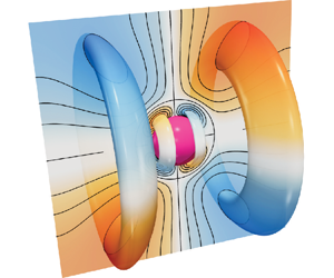
Finally, we demonstrate how gained theoretical insights translate to three-dimensional geometries characterized by multiple curvatures and distinct topology, illustrated here by means of a torus, a shape of interest due to its microfluidic properties (Chan et al. 2022) and recent bioengineered demonstrations (Dou et al. 2022). Figure 3(a) presents the streaming flow generated for a rigid torus immersed in an oscillatory flow field at $M \approx 4$. As can be seen, the highlighted recirculating flow features (inner/outer flow rings that may be used for particle manipulation) are weak for practical applications in the rigid limit. This can be remedied by increasing elasticity ($\mathrm {Cau}$), for which we indeed observe enhanced flow strengths (figure 3b,c). Finally, we highlight that to obtain a flow topology similar to that of figure 3(c), but with a rigid torus, oscillation frequencies ${\sim }4\times$ higher are necessary (supplementary material § 7), in conformity with the intuition gained via the soft-sphere streaming analysis.

Figure 3. Extension to complex bodies. Here we consider compliance-induced streaming in a soft torus, a complex shape entailing multiple curvatures and distinct topology relative to the sphere. Numerically simulated time-averaged Eulerian flow topologies for a torus of core radius $r$ and cross-sectional radius $a = r/3$, at $M \approx 4$, with varying body elasticity $\mathrm {Cau}$. (a) Rigid limit $\mathrm {Cau} = 0$, (b) $\mathrm {Cau} = 0.025$ and (c) $\mathrm {Cau} = 0.05$. The viscous fluid oscillates with velocity $V(t) = \epsilon a \omega \cos \omega t$. The torus is ‘pinned’ at the centre of its circular cross-section by a rigid toroidal inclusion of radius $0.4a$. All other physical and simulation parameters are consistent with sphere streaming (see caption of figure 2 for details).

5. Conclusion

In summary, this study improves existing three-dimensional rigid-sphere streaming theory, expands it to the case of elastic materials and further corroborates it by means of direct numerical simulations. Our work reveals, in keeping with our previous work on two-dimensional soft cylinders, an additional streaming mode accessible through material compliance and available even in Stokes flow. It further demonstrates how body elasticity strengthens streaming or enables it at significantly lower frequencies relative to rigid bodies. Finally, we show how theoretical insights extend to geometries other than the sphere, highlighting the practical generality of our theory. Overall, these findings advance our fundamental understanding of streaming flows, with potential implications in both biological and engineering domains.