Equatorial modons in thermal rotating shallow water model

Abstract

Exact steady eastward-moving vortex-dipole solutions, the equatorial modons, are constructed in the asymptotic limit of low divergence and small temperature variations in the thermal rotating shallow water (TRSW) model on the equatorial beta-plane. This regime is known to be relevant for the tropical atmosphere. The model itself is a generalization, allowing for horizontal temperature gradients, of the classical rotating shallow water model. The asymptotic modons can carry a temperature anomaly and exist also on the inhomogeneous temperature background. The modon configurations are then used to initialize numerical simulations, in order to check whether such coherent structures can exist in the full TRSW model. The results show that this is, indeed, the case. The parameter regimes and limitations on the structure of the temperature anomaly inside, in order for the modons to persist, are established. It is also shown that the modons keep their coherence even while evolving on the background of meridionally inhomogeneous temperature fields, or while interacting with sharp temperature fronts. A general scenario of disaggregation of the modons, if they are out of the stability domain, is exhibited and analysed.

1. Introduction

Rotating shallow water (RSW) model on the equatorial beta plane (a linear approximation of the Coriolis parameter valid in the vicinity of the equator) is a standard conceptual tool for analysing the large-scale dynamics of the equatorial atmosphere and ocean. The use of the model was initiated in the seminal works by Matsuno (1966), Lindzen (1967) and Gill (1980), and has become widespread since then. Obvious advantages of the model are its simplicity and, at the same time, its ability to capture essential elements of the dynamics, which allows for in-depth analytic studies and, at the same time, for high-resolution numerical investigations at low computational cost. For example, the response of the tropical atmosphere to a localized heating, which was obtained semi-analytically by Gill (1980) using this model, has become a folklore in tropical meteorology and climatology. In the same spirit, a full theory of relaxation (adjustment) of zonally elongated pressure and velocity anomalies at the equator was developed and confirmed by high-resolution numerical simulations in LeSommer, Reznik & Zeitlin (2004).

In spite of the long history of applications of the model to the tropical atmosphere, some of its important features were discovered only recently. Thus, it was shown (Rostami & Zeitlin 2019a, 2021) that coherent eastward-moving dipolar structures, the equatorial modons, exist in the model. Unlike previously known westward-moving dipolar solitons, which were also called modons (Boyd 1985) and have a large zonal-to-meridional aspect ratio (LeSommer et al. 2004), these modons have an aspect ratio of order one and the opposite sense of propagation. It was also shown in Rostami & Zeitlin (2019b) that the scenario of the equatorial adjustment is not universal, depending on the aspect ratio of the initial perturbation, among other parameters. For aspect ratios close to one, and strong perturbations accompanied by diabatic heating, equatorial modons arise in the course of the adjustment process. The equatorial modon solutions were first obtained analytically in the limit of low divergence, which is pertinent for large-scale motions of the equatorial atmosphere, as was first noticed by Charney (1963). This is why this dynamical regime was called the Charney regime in Rostami & Zeitlin (2019a). At the leading order, the equations of the model in this regime are equivalent to the barotropic quasi-geostrophic (QG) equations on the mid-latitude beta-plane, and the construction of the modon solutions straightforwardly follows the well-known procedure pioneered in the geophysical fluid dynamics context by Larichev & Reznik (1976). The corresponding analytic solution of the full RSW equations on the equatorial beta-plane is unknown, but it was shown in Rostami & Zeitlin (2019a) that, if high-resolution numerical simulations are initialized with the low-divergence regime solution, the latter quickly adjusts, by emitting inertia–gravity waves, to a coherent dipolar vortex which steadily moves eastward along the equator and keeps its shape for very long times. The situation here is similar to that with modon solutions of the full RSW equations on the $f$-plane (constant Coriolis parameter), for which the analytic solution is unknown but which can be shown to exist either by semi-analytic computer-assisted calculations (Kizner et al. 2008), or by direct numerical simulations initialized with the known QG modon which rapidly relaxes to a long-living coherent dipole by emitting inertia–gravity waves (Ribstein, Gula & Zeitlin 2010).

In spite of the above-mentioned successful applications of the RSW to the equatorial beta-plane, the model has an essential drawback as it does not allow for horizontal temperature (or potential temperature) gradients. This difficulty is usually circumvented by considering thickness in the RSW equations as a proxy for temperature. For example, the so-called weak-temperature-gradient approximation to forced-dissipative RSW (Sobel, Nilsson & Polvany 2001), which is of use in the literature, becomes – in the absence of diabatic heating and dissipation, and if considered on the equatorial beta-plane – the Charney-regime equations of Rostami & Zeitlin (2019a). Yet, there is no temperature variable as such in the model. This drawback can be removed by using, instead of the standard RSW, the so-called thermal rotating shallow water (TRSW) model which can be obtained, like the RSW model, from the primitive equations by the same method of vertical averaging and mean-field approximation, but relaxing the constraint of horizontal homogeneity of buoyancy. The TRSW model, which first appeared in O'Brien & Reid (1967) and since then has been multiply rediscovered in the literature (cf. e.g. Zeitlin (2018), Ch.14 for derivation and references), has been a subject of growing interest in recent years, both for studying observable phenomena in the ocean and atmospheres (e.g. Cho et al. 2008; Warnerford & Dellar 2014; Lahaye, Zeitlin & Dubos 2020; Holm, Luesnik & Pan 2021; Kurganov, Liu & Zeitlin 2021a), and as a test ground for numerical methods for atmospheric dynamics (e.g. Zerroukat & Allen 2015; Kurganov, Liu & Zeitlin 2021b). A forced-dissipative version of the TRSW model including the thermal effects of moist convection was constructed and tested recently in Kurganov, Liu & Zeitlin (2020a). The TRSW model in the mid-latitude $f$- or $\beta$- plane approximation admits a well-defined thermal quasi-geostrophic (TQG) approximation (Ripa 1996; Warneford & Dellar 2013). It was recently shown by Lahaye et al. (2020) that the previously mentioned classical QG modon solutions can be generalized to give thermal modon solutions of TQG. The latter can carry a thermal anomaly, in addition to the vorticity anomaly of the classical QG modons. If numerical simulations with full TRSW equations are initialized with TQG modons, these latter rapidly adjust and provide long-living coherent vortex dipoles with associated localized temperature anomalies, thus indicating, similarly to the ‘pure’ RSW case mentioned above, the existence of this kind of solution in TRSW.

In the present paper we will follow a similar strategy, i.e. we will be looking for the modon solutions of the asymptotic limit of the model, which we do find, and then will be initializing numerical simulations with these solutions, in order to check the survival of the asymptotic solutions in the full model. In this way we will demonstrate the existence in the TRSW model on the equatorial beta-plane of coherent dipolar vortices, which are moving eastward along the equator, are long lived and are carrying (or not) temperature anomalies. These solutions turn out to be very robust, decaying mainly due to dissipation, and not because of intrinsic instabilities. They keep their coherence, even propagating on the background of an inhomogeneous temperature field.

The paper is organized as follows. In § 2 we recall the TRSW model, establish its low-divergence/weak-temperature-variation limit and construct equatorial modon solutions of the latter. In § 3 we present results of numerical simulations initialized with the thus found modon configurations with various initial distributions of the temperature field. Section 4 contains a discussion of the obtained results and a sketch of the directions of further work.

2. The TRSW model and its asymptotic modon solutions

2.1. The model and the scaling

The equations of the TRSW model on the equatorial beta-plane with zonal coordinate $x$ and meridional coordinate $y$ read

(2.1) \begin{equation} \left.\begin{array}{c@{}} \partial_{t}\boldsymbol{v} + \boldsymbol{v}\boldsymbol{\cdot} \boldsymbol{\nabla} \boldsymbol{v} + \beta y \boldsymbol{\hat{z}} \wedge \boldsymbol{v} ={-}b \boldsymbol{\nabla} h - \displaystyle\dfrac{h}{2} \boldsymbol{\nabla} b,\\ \partial_{t}h + \boldsymbol{\nabla} \boldsymbol{\cdot} ( \boldsymbol{v} h) = 0,\quad \partial_{t} b + \boldsymbol{v} \boldsymbol{\cdot} \boldsymbol{\nabla} b = 0, \end{array} \right\} \end{equation}

where $\boldsymbol {\nabla } = (\partial _x, \partial _y)$, $\beta$ is the meridional gradient of the Coriolis parameter, $\boldsymbol {v}(x,y) = (u,v)$ is the horizontal velocity, $\boldsymbol {\hat {z}}$ is the unit vector in the vertical direction, $h(x,y)$ is the geopotential height and $b(x,y)$ is buoyancy. The latter is defined as $b = -g(({\theta _0 - \theta (x,y)})/{\theta _0})$ where g is the constant of gravity in the atmosphere, and as $b = g(({\rho _0 - \rho (x,y)})/{\rho _0})$ in the oceanic context, where $\theta$ and $\rho$ are, respectively, the potential temperature and density perturbations, both directly related to temperature variations, and the index $0$ denotes the background value. Both buoyancy and thickness have positive means, $B_{0}$ and $H_{0}$, respectively, defining an intrinsic velocity scale $c = \sqrt {B_{0} H_{0}}$. As is well known, there also exists an intrinsic length scale in the model, the equatorial deformation radius $L_{d} = \sqrt {{\sqrt {B_0 H_0}}/{\beta }}$.

The standard equatorial scaling consists of using $L_{d}$ and $c$ as spatial and velocity scales: $(x,y) \sim L_d = \sqrt {{c}/{\beta }}$, $(u,v) \sim c$. The time scale then is $t \sim L_d/c$, and we introduce non-dimensional deviations of thickness and buoyancy from their mean values: $b = B_0(1+\tilde {b})$, $h= H_0(1+\tilde {h})$. The TRSW equations scaled in this way read, with non-dimensional variables marked by tilde,

(2.2a)\begin{gather} {\frac{\partial{\tilde{\boldsymbol{v}}}}{\partial{t}}} + \tilde{\boldsymbol{v}}\boldsymbol{\cdot} \boldsymbol{\nabla}{\tilde{\boldsymbol{v}}} + y \hat{\boldsymbol{z}} \wedge{\tilde{\boldsymbol{v}}} ={-}(1+\tilde{b})\boldsymbol{\nabla}{\tilde{h}} - \frac{(1+\tilde{h})}{2}\boldsymbol{\nabla}{\tilde{b}}, \end{gather}

(2.2b)\begin{gather}{\frac{\partial{\tilde{h}}}{\partial{t}}} + \boldsymbol{\nabla}\boldsymbol{\cdot}{((1+\tilde{h})\tilde{\boldsymbol{v}})} = 0, \end{gather}

(2.2c)\begin{gather}{\frac{\partial{\tilde{b}}}{\partial{t}}} + \tilde{\boldsymbol{v}}\boldsymbol{\cdot}\boldsymbol{\nabla}{\tilde{b}} = 0. \end{gather}

This system, with the addition of dissipative terms, will be implemented in the numerical simulations in § 3. However, in order to construct the asymptotic regime and modon solutions we will use, following Rostami & Zeitlin (2019a), another scaling: a single spatial and a single velocity scale, $(x,y) \sim L$ and $(u,v) \sim U$, and the eddy turnover time scale $t \sim L/U$. With these scales being introduced, the non-dimensional parameters, the Froude and Burger numbers, can be defined in the standard way

(2.3a,b)\begin{equation} Fr =\frac{U}{c}, \quad Bu = \frac{L_d^2}{L^2}. \end{equation}

We also introduce the parameters $\gamma$ and $\lambda$, measuring the amplitude of, respectively, buoyancy and thickness perturbations: $b = B_0(1+\gamma \tilde {b})$, $h= H_0(1+\lambda \tilde h)$. Thus scaled equations (2.1) read

(2.4a)\begin{gather} {\frac{\partial{\tilde{\boldsymbol{v}}}}{\partial{t}}} +\tilde{\boldsymbol{v}}\boldsymbol{\cdot}\boldsymbol{\nabla}{\tilde{\boldsymbol{v}}} + \frac{1}{Fr Bu}y\boldsymbol{z}\wedge{\tilde{\boldsymbol{v}}} ={-}\frac{\lambda}{Fr^{2}} \boldsymbol{\nabla}{\tilde{h}} - \frac{\gamma}{2 Fr^2} \boldsymbol{\nabla}{\tilde{b}} - \frac{\gamma\lambda\tilde{b}}{Fr^2} \boldsymbol{\nabla}{\tilde{h}} - \frac{\lambda\gamma\tilde{h}}{2 Fr^2} \boldsymbol{\nabla}{\tilde{b}}, \end{gather}

(2.4b)\begin{gather}\lambda{\frac{\partial{\tilde{h}}}{\partial{t}}} + \boldsymbol{\nabla}\boldsymbol{\cdot}{((1 + \lambda\tilde{h})\tilde{\boldsymbol{v}})} = 0, \end{gather}

(2.4c)\begin{gather}{\frac{\partial{\tilde{b}}}{\partial{t}}} + \tilde{\boldsymbol{v}}\boldsymbol{\cdot}\boldsymbol{\nabla}{\tilde{b}} = 0. \end{gather}

2.2. Charney/weak-temperature-gradient regime

Following Rostami & Zeitlin (2019a), we now consider a dynamical regime where the deviations of thickness are small: $\lambda \rightarrow 0$. (It is probably worth noting that such a regime is called ‘long wave’ in oceanography cf. Gill 1982). We will suppose that buoyancy variations are also small: $\gamma \rightarrow 0$, which is consistent with the observed overall weak temperature gradients in the equatorial region (cf. e.g. Sobel et al. (2001), and references therein). We will suppose that $\lambda$ and $\gamma$ are of the same order of magnitude (although this assumption is not crucial for what follows), and put $\gamma = 2 \lambda$ without loss of generality. If we suppose then, again following Rostami & Zeitlin (2019a), that $Fr^{2} = \mathcal {O}(\lambda )$, we get

(2.5a)\begin{gather} {\frac{\partial{\tilde{\boldsymbol{v}}}}{\partial{t}}} +\tilde{\boldsymbol{v}}\boldsymbol{\cdot}\boldsymbol{\nabla}{\tilde{\boldsymbol{v}}} + \bar{\beta}y \boldsymbol{\hat{z}}\wedge{\tilde{\boldsymbol{v}}} ={-}(1 + 2Fr^2\tilde{b})\boldsymbol{\nabla}{\tilde{h}} - (1 + Fr^2\tilde{h})\boldsymbol{\nabla}{\tilde{b}}, \end{gather}

(2.5b)\begin{gather}Fr^2{\frac{\partial{\tilde{h}}}{\partial{t}}} + \boldsymbol{\nabla}\boldsymbol{\cdot}{((1 + Fr^2\tilde{h})\tilde{\boldsymbol{v}})} = 0, \end{gather}

(2.5c)\begin{gather}{\frac{\partial{\tilde{b}}}{\partial{t}}} + \tilde{\boldsymbol{v}}\boldsymbol{\cdot}\boldsymbol{\nabla}{\tilde{b}} = 0, \end{gather}

where we introduced the notation $\bar {\beta } = {1}/{Fr Bu}$. At the leading order in $Fr^{2}$ this gives

(2.6a)\begin{gather} {\frac{\partial{\boldsymbol{v}}}{\partial{t}}} +\boldsymbol{v}\boldsymbol{\cdot} \boldsymbol{\nabla} \boldsymbol{v} + \bar{\beta} y\,\boldsymbol{\hat{z}} \wedge{\boldsymbol{v}} ={-}\boldsymbol{\nabla}{h} - \boldsymbol{\nabla}{b}, \end{gather}

(2.6b)\begin{gather}\boldsymbol{\nabla}\boldsymbol{\cdot}{\boldsymbol{v}} = 0, \end{gather}

(2.6c)\begin{gather}{\frac{\partial{b}}{\partial{t}}} + \boldsymbol{v} \boldsymbol{\cdot} \boldsymbol{\nabla}{b} = 0, \end{gather}

where we omitted tildes for simplicity of notation. Equation (2.6b) allows us to introduce a streamfunction $u = -{\partial \psi }/{\partial y}, v = {\partial \psi }/{\partial x}$ and to rewrite (2.6) as follows:

(2.7a)\begin{gather} \partial_t{{\nabla}^2{\psi}} + J(\psi,{\nabla}^2{\psi}) + \bar{\beta}\partial_x{\psi} = 0, \end{gather}

(2.7b)\begin{gather}\partial_{t}{b}+ J(\psi,b) = 0. \end{gather}

2.3. Asymptotic modon solutions

Equation (2.7a) coincides with the equation for the streamfunction in the Charney regime obtained in Rostami & Zeitlin (2019a), and is not modified by the effects of variable buoyancy. Thus, our derivation shows that, in the asymptotic regime, buoyancy behaves as a passive scalar which is advected by the flow according to (2.7b). This means that the equatorial modon solutions obtained in this regime in Rostami & Zeitlin (2019a) are also valid here and, whatever they are, the buoyancy is just advected by their velocity field. We give below a brief description of the procedure of finding the modon solutions of (2.7a), which literally follows Rostami & Zeitlin (2019a).

Looking for solutions of (2.7a) moving zonally with constant velocity $V$: $\psi = \psi (x-Vt, y)$, we get

(2.8)\begin{equation} J\left(\psi + Vy, {\nabla}^2{\psi} + \displaystyle \frac{1}{Fr Bu}y\right) = 0, \Rightarrow {\nabla}^2{\psi} + \displaystyle \frac{1}{Fr Bu}y = F(\psi + Vy), \end{equation}

where $F$ is an arbitrary function. The $(x,y)$ plane is divided by a circle of radius $r_{0}$ into interior and exterior domains, and $F$ in (2.8) is assumed to be a linear function $F(\psi+Vy) \propto\psi+Vy$, although with different constants (slopes), in each of them, which will be denoted $\alpha ^{2}$ and $p^{2}$, respectively. The streamfunction in the interior domain is given by solutions of the following linear inhomogeneous equation:

(2.9)\begin{equation} {\nabla}^2{\psi_{in}} + \alpha^2\psi_{in} ={-}\left(\frac{1}{FrBu} + \alpha^2~V\right)y, \end{equation}

with $\alpha$ to be determined. Its solution is a superposition of a general solution of the corresponding homogeneous equation, and of the particular solution of the inhomogeneous equation which is proportional to $y = r \sin \theta$, where $(r, \theta )$ are polar coordinates. The homogeneous equation is solved in polar coordinates by the method of separation of variables, assuming a dipolar structure $\sim \sin \theta$ for consistency with the inhomogeneous solution, which results in a Bessel differential equation in $r$. Only a regular at $r =0$ Bessel function is physically acceptable as a solution.

A condition of decay at infinity allows us to fix the constant in the exterior domain

(2.10)\begin{equation} {\nabla}^2{\psi_{out}} = p^2\psi_{out}, \quad p^2 = \frac{1}{Fr Bu V}. \end{equation}

Solutions are sought in polar coordinates by the method of separation of variables, assuming the same angular structure, for consistency, which leads to the equation for modified Bessel functions. The solution in the whole plane is then given by

(2.11)\begin{equation} \psi(r, \theta) = \begin{cases} \displaystyle \frac{-Vr_0}{K_1(pr_0)}K_1(pr)\sin(\theta), & r > r_0 \\ \displaystyle \frac{1}{\alpha^2FrBuJ_1(\alpha r_0)}r_0 J_1(\alpha r)\sin(\theta) - \displaystyle \frac{\left(\dfrac{1}{FrBu} + \alpha^2V\right)}{\alpha^2}r\sin(\theta), & r < r_0 \end{cases}, \end{equation}

where $K_{1}$ and $J_{1}$ are, respectively, the modified and the ordinary Bessel functions, and $p$ is given by (2.10).

The last step consists of matching the inner and outer solutions across the separatrix $r = r_{0}$, in order to ensure the continuity of $\psi$ and its derivatives. This leads to the following transcendental equation:

(2.12)\begin{equation} \frac{1}{p} \frac{K_2(p r_0)}{K_1(p r_0)} ={-}\frac{1}{\alpha}\frac{J_2(\alpha r_0)}{J_1(\alpha r_0)}. \end{equation}

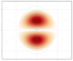
This equation allows us to determine the value of $\alpha$ for each value of $p$, i.e. for each value of $V$, $r_0$, $Fr$ and $Bu$, and thus allows us to completely determine the function $\psi$ in (2.11) in terms of these four parameters. Equation (2.12) has multiple roots, with the first, strictly positive one, giving a dipolar (modon) solution with rightward (eastward) propagation. The zeros of (2.12) were found numerically using the SciPy optimize.fsolve routine (https://docs.scipy.org/.) It uses the subroutine HYBRD of the MINPACK library, which determines the roots of a function using an iterative method (a modification of the Powell hybrid method). In the simulations below, $V$ and $r_0$ are taken to be equal to $0.5$ in dimensionless units. An example of such solutions is presented in figure 1.

Figure 1. Streamfunction ($\psi$) of a modon with $Fr = 0.1$, $Bu = 1$, $V = 0.5$ and $r_0 = 0.5$.

Let us recall that the streamfunction of the thus found modon solution is the same as in the equatorial modons in RSW in the Charney regime on the equatorial beta plane (Rostami & Zeitlin 2021), the difference between the modons in the two models residing in the thickness and buoyancy fields. Indeed, once the streamfunction of the solution is found, and the buoyancy profile determined (see below), the distribution of the sum $h + b$ can be determined by solving the following Poisson equation for this quantity, obtained by taking the divergence of (2.6a):

(2.13)\begin{equation} - {\nabla}^2{(h + b)} = 2(\psi_{yx})^2 - 2\psi_{xx}\psi_{yy} - \bar{\beta}y{\nabla}^2{\psi} - \bar{\beta}\psi_y. \end{equation}

An essential difference between (2.7) and the TQG equations (Ripa 1996; Warneford & Dellar 2013), which were used for constructing modon solutions by Lahaye et al. (2020), is that the former are decoupled, and thus the modons exist for any distribution of buoyancy. The only role of buoyancy in the solution is to determine the corresponding thickness profile, as follows from (2.13): once a distribution of $b$ is chosen, with $\psi$ corresponding to the modon, the solution of the resulting Poisson equation determines $h$, and therefore the complete structure of the modon, for any $b$. However, if we want to have a buoyancy anomaly transported by the modon, i.e. moving with the same velocity, we then have to suppose that

(2.14)\begin{equation} J(\psi + V y,b) = 0, \Rightarrow b = G(\psi + V y), \end{equation}

where $G$ is an arbitrary function of the streamfunction in the co-moving frame. The simplest choice is to take $G$ to be linear in the inner domain, and zero in the outer domain, although more general distributions will be considered in § 3.2.2 below. Both symmetric and antisymmetric, with respect to equator buoyancy, anomalies inside the modon can be obtained in this way by taking $G \propto |\psi + V y|$ or $G \propto \psi + V y$, respectively. We will mostly display below the results for the more physically relevant sign-definite distribution

(2.15)\begin{equation} G = \sigma |\psi + V y|, \end{equation}

with different values of $\sigma$.

Obviously, in the full TRSW model the decoupling of buoyancy and velocity is not operational. Furthermore, the derivation of the asymptotic models discards, together with inertia–gravity waves, Kelvin and Yanai (mixed Rossby–gravity) waves, which are ubiquitous features of the large-scale equatorial dynamics. Therefore, in this context it is especially important to check the evolution of the TRSW system initialized with asymptotic modon solutions, in order to see if the modons survive in the presence of the full set of equatorial waves. Such investigation is presented in the next section.

3. Equatorial modons as seen in numerical simulations with the TRSW model

3.1. Numerical set-up

Numerical simulations were performed with the Dedalus library (Burns et al. 2020) for Python. Dedalus is a spectral (in spatial variables) code resolving partial differential equations, with several possible choices for time integration. In our simulations, a split-explicit fourth-order Runge–Kutta method has been used for this purpose. Periodic boundary conditions were imposed in order to implement the Dedalus code, and (2.2) obtained with the standard equatorial scaling were used. However, the momentum equation (2.2a) contains a non-periodic Coriolis term, which is a linear function of the meridional coordinate. Periodic extension of the function $y$ entering this term is a discontinuous sawtooth function, which is not suitable for numerical treatment. That is why the jump at the zonal boundaries of the computational domain was smoothed using a rapidly decreasing to zero at the boundary smooth function, which ensures periodicity (see the details in Appendix A). The modified $y$ function is denoted by $\hat y$ below. In order to prevent numerical oscillations during the simulations, dissipation in the form of a hyper-viscosity in the momentum and diffusivity in the buoyancy equation has been introduced. These terms were tuned to be sufficiently large to prevent any numerical oscillations, but were as small as possible to avoid a too rapid dissipative damping. A nudging term, $N$, of relaxation to zero type, was also added for height and buoyancy anomalies in the vicinity of the top and bottom boundaries, in order to damp waves crossing these boundaries, and thus avoid wave reflection and interference with the vortex centred at the equator (see Appendix A). The computational domain was chosen to be wide enough to hold off as far as possible the effects of interpolation of the Coriolis term and of the nudging. The system of equations implemented in the numerical scheme is thus given by

(3.1a)\begin{gather} {\frac{\partial{\tilde{\boldsymbol{v}}}}{\partial{t}}} + \tilde{\boldsymbol{v}}\boldsymbol{\cdot}\boldsymbol{\nabla}{\tilde{\boldsymbol{v}}} + \hat y\boldsymbol{\hat{z}} \wedge{\tilde{\boldsymbol{v}}} ={-}(1+\tilde{b})\boldsymbol{\nabla}{\tilde{h}} - \frac{(1+\tilde{h})}{2}\boldsymbol{\nabla}{\tilde{b}} - ({-}1)^n \nu \varDelta^n(\tilde{\boldsymbol{v}}), \end{gather}

(3.1b)\begin{gather}{\frac{\partial{\tilde{h}}}{\partial{t}}} + \boldsymbol{\nabla}\boldsymbol{\cdot}{((1+\tilde{h})\tilde{\boldsymbol{v}})} ={-}N(\tilde{h},y), \end{gather}

(3.1c)\begin{gather}{\frac{\partial{\tilde{b}}}{\partial{t}}} + \tilde{\boldsymbol{v}}\boldsymbol{\cdot}\boldsymbol{\nabla}{\tilde{b}} ={-}\kappa\varDelta(\tilde{b}) -N(\tilde{b},y). \end{gather}

Here, $\varDelta$ denotes the Laplacian, $\nu$ and $\kappa$ are viscosity and diffusivity coefficients, respectively, and we performed simulations with various values of the integer $n$ defining the order of the hyperviscosity operator, with $n =1$ corresponding to Newtonian viscosity.

3.1.1. Benchmarks and initializations

As a benchmark of the code, which is not especially designed for shallow water models, we started our numerical investigations with the standard problem of adjustment of an elongated thickness anomaly at the equator. The simulation was performed in a domain of $50 \times 15$ ($L_x \times L_y$) with a resolution of $1280 \times 384$. The results, which are shown in figure 2, confirm, qualitatively and quantitatively, those of LeSommer et al. (2004) which were obtained with a dedicated RSW code. Our generic numerical code cannot resolve shocks in shallow water, which are inherent e.g. to the propagation of equatorial Kelvin waves, producing the so-called Kelvin fronts (Fedorov & Melville 2000; LeSommer et al. 2004). Nevertheless, it does reproduce the corresponding sharp gradients, as clearly seen in the figure. We have also run another benchmark test, the adjustment of a thermal anomaly at the equator, which is specific for TRSW, and again found qualitative and quantitative agreement with the results obtained with a dedicated TRSW code (Kurganov et al. 2020a) (not shown).

Figure 2. Evolution of vorticity, in units of ${c}/{L_d}$, and height, in units of $H_0$, during the adjustment of an initial zonally elongated height anomaly with magnitude $-0.1 H_0$, $Bu = 1$. Time in units of ${1}/{\beta L_d}$, length in units of $L_{d}$. Notice the large difference between meridional and zonal scales in all panels. (a,b) $t =0$, (c,d) $t = 5$, (e,f) $t =15$.

3.1.2. Initial conditions for the simulations

In order to initialize the simulations following the evolution of the asymptotic modon solution, we use the streamfunctions of the modon in the outer and inner regions in order to determine the velocity field, then choose the initial buoyancy field, and perform numerically the inversion in (2.13) in order to find the initial $h$ (see Appendix B). We should emphasize that, although the initialization with flat $h$ and the modon velocity field produces a rapid adjustment to a coherent dipole, as was shown in Rostami & Zeitlin (2019a), the initialization with a pre-adjusted $h$ field drastically reduces the amount of emitted inertia–gravity waves and speeds up the adjustment process, as we checked. We tested different initial configurations of buoyancy, with positive and negative buoyancy anomalies inside the modon's radius $r_{0}$, but also with positive and negative dipolar buoyancy anomalies inside the modon, of the same form as the modon's streamfunction. We also tested the evolution of the modon on a background of a zonally homogeneous meridionally symmetric temperature (buoyancy) field with a maximum at $y = 0$, roughly mimicking the observed zonally and time-averaged temperature field at the equator, and simulated an encounter of the modon with a temperature front across the equator. It should be emphasized that, if a non-trivial mean buoyancy field without a mean flow is introduced to the problem, it should be accompanied by a compensating thickness field, in order to remain stationary and avoid its proper evolution (adjustment) which would ‘pollute’ the interaction with a modon. This means that the right-hand side of (2.2a) or, in the asymptotic regime, the right-hand side of (2.6a) should be zero. In all simulations presented below, the spatial resolution was $256 \times 256$, and the size of the domain was $L_x = L_y = 8$. The simulations were run for very long times: several hundreds of non-dimensional units. The values of $Fr$ and $Bu$ in the simulations presented below were $0.1$ and $1$, respectively, unless otherwise stated.

3.2. Results of numerical simulations

3.2.1. Modons in the absence of an inhomogeneous buoyancy background

We start with the simulations with no background buoyancy field, initializing them, as described above, with the velocity obtained from the streamfunction of the modon (2.11), and a buoyancy field proportional to the modulus of the streamfunction in the comoving frame. We present in figure 3 the initial and final stages of the evolution of the modon with a negative buoyancy anomaly of the form of (2.15) with $\sigma = 10$ (giving an initial buoyancy field of intensity $-0.09$). In this and subsequent illustrations, we show only a part of the computational domain, which is much larger in the meridional direction, as explained above. As already mentioned, at the initial stages of the evolution an adjustment process with emission of inertia–gravity waves and a weak signature of a Kelvin wave takes place (not shown). These waves are of feeble intensity, are rapidly dissipated and their interactions with the modon due to returns, with periodic boundary conditions, are insignificant. As seen in the figure, the modon keeps running eastward without notable change of its vorticity, thickness and buoyancy anomalies. For comparison, the position of the separatrix at $r=0.5$ of the corresponding solution of the asymptotic model (which, we recall, propagates at the velocity $Fr/2$ exactly preserving its form) is indicated in this and subsequent figures. It shows that the adjusted modon propagates at a slightly reduced velocity compared with the asymptotic solution. In the course of its evolution, the modon develops a multipolar divergence pattern of weak intensity, which was also observed for mid-latitude RSW modons (Ribstein et al. 2010). Rather surprisingly, no traces of the thermal instability, which is typical for TRSW vortices (Gouzien et al. 2017) and was observed in mid-latitude TRSW modons (Lahaye et al. 2020), can be distinguished.

Figure 3. Evolution of thickness, buoyancy, vorticity and divergence anomalies of the modon with initial negative buoyancy anomaly of intensity $0.09$ with hyperviscosity of the order $n=4$, and viscosity coefficient $\nu = 10^{-16}$. $t = 0$ (a,c,e,g), $t = 290$ (b,d,f,h). The black dashed line superimposed on the vorticity field indicates the position at $r=.5/\sqrt {Bu}$ of the separatrix of the asymptotic modon solution which propagates with the speed $0.5Fr$.

The simulation with an initial modon with a positive buoyancy anomaly of the same form and intensity gives similar results, which are presented in figure 4, although the lag with respect to asymptotic solution is more pronounced. Simulations with the same initial conditions, but with increasing dissipation (larger $\nu$ and/or smaller order of (hyper-)viscosity $n$) give very close results until a threshold of sufficiently strong dissipation is reached ($\nu \sim 10^{-4}$ with $n=1$), when the evolution of the modon changes qualitatively: the intensity of its component vortices diminishes, the distance between their centres increases and the speed of propagation of the whole system decreases until it stops and engages in the backward (westward) motion. Such evolution can be easily explained by the fact that the mutual interaction between the vortices weakens as their intensities decrease due to dissipation, allowing the phenomenon of beta drift to affect the evolution of the vortices. We should recall that the beta drift is due to formation of beta gyres, that is, zones of opposite vorticity at the sides of the vortex, which are pushing a cyclonic vortex in north–west (south–west) direction in the northern (southern) hemisphere, leaving a Rossby-wave tail behind, a fact which is well known in QG models, e.g. Reznik & Grimshaw (2001). In the shallow-water model, the emission of inertia–gravity waves accompanies this non-stationary process. Thus, under the joint influence of dissipation and Rossby and inertia-gravity wave emission, the pair of vortices is gradually transformed into a system of Rossby and inertia–gravity waves, as shown in figure 5 where beta gyres are also visible in panel (e). It is worth recalling in this context that the very existence of the equatorial modon as a coherent structure in the RSW model, which contains a plethora of equatorial waves, is due to the fact that its propagation speed does not match that of westward-propagating equatorial Rossby waves having a similar vorticity structure, nor that of eastward- and westward-propagating equatorial inertia–gravity waves, so a resonance between the modon and linear waves is impossible. (Fast eastward-propagating Kelvin waves having an orthogonal meridional structure, as well as Yanai waves, are standing apart.) Once the modon decelerates and stops due to dissipation, its transformation into a wave system is inevitable, and this is what is observed in the figure.

Figure 4. Same as in figure 3 but with initial positive buoyancy anomaly of intensity $0.09$.

Figure 5. Thickness, buoyancy and vorticity anomalies at intermediate stages of the simulation initialized with the same configuration as in figure 4, with Newtonian viscosity $n=1$, and viscosity coefficient $\nu = 10^{-4}$. (a,c,e): $t = 80$, (b,d,f): $t = 140$.

We finally discuss the evolution of the modon initialized with the antisymmetric buoyancy anomaly inside, which is proportional to the co-moving streamfunction, and not to its modulus. As follows from figure 6, such a modon does not survive in the full TRSW model. The dipole starts distorting and wiggling around its axis of propagation, which eventually leads to the separation of the two poles of vorticity, a halt of the dipole and a reverse motion. An in-depth investigation of the mechanism leading to the destabilization of the modon is beyond the scope of the manuscript. Nonetheless, we note that, this destabilization, unlike the one caused by strong dissipation as reported above, appears to be triggered by an intrinsic instability mechanism. Indeed, below a certain value of the hyperviscosity coefficient ($10^{-7}$ with a second order hyperviscosity) – above which the above-reported dissipation-induced destabilization dominates the evolution of the modon – the rate of destabilization of the modon accelerates slightly with decreasing hyperviscosity (the minimal value of hyperviscosity tested is $10^{-9}$ – again for second order hyperviscosity). Moreover, we have checked that flipping the sign of the initial distribution of the buoyancy with respect to the equator leads to the same, but mirror-symmetric, destabilization of the modon, confirming the decisive role of the antisymmetric nature of the buoyancy distribution.

Figure 6. Evolution of vorticity and buoyancy fields in a simulation initialized with a modon with antisymmetric buoyancy. (a,b) $t =0$, (c,d) $t = 70$, (e,f) $t =120$.

To gain some insight into this intrinsic destabilization mechanism, we calculated the exchanges of the $y$-component of momentum density $m_y=(1+\tilde h)v$ across the axis of the modon, by computing the various terms of the momentum equation, which reads (omitting the dissipation and nudging terms)

(3.2)\begin{equation} \partial_t{m_y} + \boldsymbol{\nabla}\boldsymbol{\cdot}(\boldsymbol{v}m_y) + ym_x + \partial_y\left(\frac{(1+\tilde h)^2(1+\tilde b)}{2}\right) = 0. \end{equation}

These terms, and in particular their evolution along the axis $y=0$, which diagnoses the destabilization of the modon, are shown in figure 7. Note that, by construction, the Coriolis term vanishes on the axis $y=0$ and is not shown in the figure. Both the initial antisymmetric distribution of the buoyancy, and thus the asymmetric distribution of $h$, are associated with a non-zero pressure gradient term (last term in (3.2)). After the initial adjustment, the different terms of this equation become non-zero and not zonally sign definite, as well as their sum. As seen in the Hovmöller diagram (figure 7c), a wave-like perturbation propagates along the $y=0$ axis, and amplifies in time. This reflects the fact that the modon starts distorting and meandering about its initial axis of propagation, which ultimately leads to its dislocation. This perturbation corresponds to the pattern of meridional momentum tendency shown in panel (d) of the figure.

Figure 7. Various terms entering the $y$-momentum balance equation evaluated along the axis at $y=0$, and $t=0$ (a), $t=4$ (b), as well as the sum of these terms yielding the $y$-momentum tendency evaluated at $y=0$ (Hovmöller plot, c) and in the $(x, y)$ plane at $t=4$ (d). In the former, the displacement of the asymptotic modon (at speed $0.5 Fr$) is indicated by the black dashed line, while the green dashed line shows the propagation speed $c=0.1$, which agrees with the apparent phase velocity of the disturbance. In the latter, the position of the modon (dashed) is marked by the vorticity isoline at $\pm 0.2$.

It should be stressed that, by construction, all the terms of the $y$-momentum in the case of the modon with a symmetric buoyancy anomaly distribution are initially zero. We checked that their amplitude remains very weak (below $10^{-9}$, compared with typical values of order $10^{-2}$ in figure 7) during the propagation of the dipole, while the overall pattern of momentum tendency is very similar to the one observed in the unstable configuration at the early stages (figure 7d).

A hint as to the intrinsic reason for the destabilization of the modon with antisymmetric buoyancy distribution inside, which leads to the meridional momentum flux across the axis as just illustrated, comes from the fact that the argument of non-resonance with equatorial waves put forward above to explain the longevity of a symmetric modon does not hold here. Indeed, as is well known, (cf. e.g. Zeitlin 2018), there is a spectral gap between symmetric in $y$ Rossby and inertia–gravity waves, which is filled in by the antisymmetric in $y$ Yanai wave, which has in addition a maximum of the meridional velocity at the equator. Thus, while the development of a Yanai wave cannot occur in a modon with symmetric buoyancy distribution, since all fields are symmetric in this case, such a process is not forbidden anymore in a modon with an antisymmetric distribution of buoyancy.

3.2.2. Modons in the presence of zonally homogeneous background buoyancy

As is well known, the zonally and time-averaged potential temperature, and hence buoyancy, has a maximum at the equator in the atmosphere. To consider the modon evolution in such more realistic environment we added a background buoyancy distribution in a form of a Gaussian function in $y$: $b^{bg} = 0.1 \, \textrm {e}^{-y^2}$. As was explained above, the construction of the modon solution in the asymptotic regime is possible for any buoyancy distribution. We thus generalized the procedure of computation of the buoyancy distribution, as compared with the previous case (2.15). Considering again the external ($r \geq r_0$) and internal ($r \leq r_0$) subdomains, one has far away from the modon

(3.3)\begin{equation} G_{out}(Vy) = b^{bg}(y) \Rightarrow G_{out}: x \mapsto b^{bg}(x/V),\quad r\geq r_0. \end{equation}

In the interior, we keep a linear function of $\varPsi +Vy$, ensuring continuity of the buoyancy profile at $r=r_0$ where $\psi +Vy=0$, which gives

(3.4)\begin{equation} G_{in}(\psi+Vy) = \kappa|\psi+Vy|+b^{bg}(0). \end{equation}

We then computed the corresponding thickness of the initial configuration as explained above. The simulation initialized in this way (with $\kappa =-10$, as in figure 3) shows that the modon perfectly keeps its coherence, as follows from figure 8.

Figure 8. Initial and late stages of the evolution of the modon with positive buoyancy anomaly inside, superimposed onto a zonally symmetric stationary background buoyancy of Gaussian form in the meridional direction. Here, $n = 2$, $\nu = 10^{-8}$. Panels show $t = 0$ (a,c,e) and $t = 295$ (b,d,f).

3.2.3. Interactions of modons with a temperature/buoyancy front

An advantage of the TRSW model, as compared with the standard RSW, is the possibility of treating temperature fronts, which are common in the oceans and in the atmosphere. We show in this subsection how the TRSW modons interact with such fronts. As already explained, the buoyancy anomaly, e.g. a front, in order to be stationary should be accompanied by compensating thickness anomaly. So we take a straight buoyancy front, and put it at a distance from the initial modon across the equator. In order to respect the periodic boundary conditions in the zonal direction we take, in fact, a double front, i.e. a meridional band of positive or negative buoyancy. This initial configuration is shown in figure 9.

Figure 9. Initial configuration for the simulation of modon–front interaction.

The eastward-propagating modon hits this double front after some time but, surprisingly, remains coherent and practically intact, passing through, as follows from figure 10, the only sensible result of the encounter being a deformation of the front, but not of the modon, due to the entrainment. The process then repeats itself, due to periodicity of the domain.

Figure 10. Evolution of thickness and buoyancy anomalies during multiple encounters of a modon with a positive buoyancy anomaly of intensity $0.09$ inside with a meridional double temperature front. Here, ${n=2}, {\nu=10^{-8}}$. (a,b) $t = 70$, (c,d) $t = 140$, (e,f) $t = 210$, (g,h) $t = 280$.

The interaction of the same modon with a meridional band of negative buoyancy of the same width goes in the same way, and the same is true for a modon with negative buoyancy inside interacting either with a positive or with a negative meridional buoyancy band (not presented).

3.2.4. Dependence on Froude and Burger numbers

The derivation of the asymptotic modon solution in § 2.3 was based on the smallness of the Froude number $Fr$, and the previously displayed results corresponded to $Fr=0.1$. We checked, however, what happens if the Froude number of the initial configuration increases, which corresponds to increasing $V$ in the asymptotic modon solution. We found that, up to and including $Fr=0.3$, the initializations with asymptotic modons with a symmetric buoyancy anomaly inside still give coherent long-living structures, as in the examples above, although the initial adjustment produces stronger inertia–gravity waves, as clearly seen in the divergence field in figure 11. Beyond that value, the initial adjustment becomes very intense and produces small-scale structures which engender numerical difficulties. We should reiterate that our code is not specially designed to resolve shocks, which become ubiquitous in shallow-water models at $Fr = \mathcal {O}(1)$, including the TRSW model, as was shown in Kurganov, Liu & Zeitlin (2020b). In fact, the local Froude number $F_{loc} = max(v/c)$ reaches the value $0.96$ at $Fr = 0.4$ (and even $1.11$ using a local $c=\sqrt {(1+\tilde h)(1+\tilde b)}$), which means that the flow becomes supercritical (‘supersonic’). In such a type of regime, the modons themselves can couple with shocks and form so-called shock modons (Lahaye & Zeitlin 2012). The present code does not allow for reliable numerical investigation of such regimes which are, in addition, not very realistic in the equatorial atmosphere, at least on Earth.

Figure 11. Evolution of a modon with $Fr=0.3$ (without buoyancy anomaly), as seen in the vorticity field (a,b) and divergence (c,d) fields. The left column shows the initial adjustment at $t=2$ with strong inertia–gravity wave emission visible in the divergence field, and the right column shows the adjusted state, to be compare with the modon with $Fr=0.1$ shown in figure 3. Colours are saturated. (a,c) $t = 2$, (b,d) $t = 48$.

The Burger number enters the dynamical equations in the Charney/weak-temperature-variation regime (2.7) only through the non-dimensional gradient of the Coriolis parameter $\bar {\beta }$, which is, in fact, nothing other than the well-known Rhines parameter governing the transition between Rossby-wave and vortex regimes on the beta-plane (Rhines 1979). At a fixed Froude number, smaller $Bu$ corresponds to larger $\bar {\beta }$, and vice versa. On this ground, we can expect that, at small $Bu$, the initial asymptotic modon would give rise to a Rossby-wave packet. This is, indeed, what happens, as follows from figure 12. As seen in the figure, the modon starts moving eastward, but slows down, with its poles undergoing meridional separation, then stops and engages in a reverse westward motion, being gradually transformed in a Rossby-wave train. This scenario is reproduced, but accelerated, at $Bu= 0.1$ and the same value of $Fr$ (not shown), while at $Bu >1$ a coherent, but more compact, modon emerges.

Figure 12. Comparative evolution of the initial asymptotic modon (with no buoyancy anomaly), as seen in the vorticity field at $Bu = 1$ (a,c,e) and at $Bu = 0.25$ (b,d,f). Here, $Fr = 0.1$. (a,b) $t = 0$, (c,d) t = 50, (e,f) $t = 100$.

4. Discussion and perspectives

We constructed asymptotic modon solutions of the TRSW equations on the equatorial $\beta$-plane in the limit of low divergence and small temperature perturbations. We showed that, if these solutions are injected as initial conditions in the numerical simulations with the full TRSW equations, they give rise to long-lived coherent dipolar vortices, steadily moving along the equator and keeping their form, which remains close to asymptotic modons if their Froude number is sufficiently small, their Burger number is of the order of one or larger and viscosity and diffusivity are sufficiently small. Several features of these structures are worth emphasizing. First, their coherence and longevity are not sensitive to the sign of the buoyancy anomaly they can carry, provided it is symmetric with respect to the equator, and they can persist on a background of meridionally inhomogeneous mean buoyancy. Moreover, the modons remain coherent even after encountering sharp temperature (buoyancy) fronts. Second, a characteristic for TRSW vortices, thermal instability, first described by Gouzien et al. (2017) on the mid-latitude $f$-plane, and then studied e.g. by Beron-Vera (2021b) and Kurganov et al. (2021b), seems to be suppressed, or at least is much less pronounced, on the equatorial $\beta$-plane. Additional, more detailed investigations, which are beyond the scope of the present work, are needed to understand whether they are under-resolved in our generic numerical scheme, or genuinely damped by the beta effect. Third, the initial modons, if they are too large – i.e. with sufficiently small Burger numbers – or are subject to strong enough dissipation, disaggregate following a seemingly universal scenario: the initially eastward-moving modon decelerates, and at the same time its poles separate in the meridional direction, until it stops and engages in the reverse, westward motion, gradually becoming an equatorial Rossby-wave packet. If the initial buoyancy distribution is not symmetric with respect to the equator, deviations of the zonal direction of propagation precede the separation of the poles, before they halt, reverse motion and disperse.

As illustrated above, the TRSW model allows one to study interaction of vortices, modons in the present case, with temperature fronts and other temperature anomalies. As already mentioned in the Introduction, the TRSW is being used for modelling of planetary atmospheres. The existence of the equatorial modons in TRSW can be exploited in this context. It was recently shown that it allows one to capture such non-trivial elements as the foehn effect (Kurganov et al. 2021a) if topography is included in the model. Inclusion of topography is straightforward, and it would be instructive to study the interaction of the thermal equatorial modons with topographic features which are abundant in the equatorial region of the Earth (the Maritime Continent, various islands and continental coasts).

Moreover, as TRSW modons (Lahaye et al. 2020) were successfully invoked for explaining the observed surface vortex dipoles in the ocean at mid-latitudes (Hughes & Miller 2017), the present study suggests that similar structures may exist in the equatorial ocean. We should recall in this context that, historically, the TRSW model was introduced to oceanography as a model for the oceanic mixed layer (McCreary, Kundu & Molinari 1993; Young 1994).

The next steps in understanding the relevance of the discovered TRSW modons to the dynamics of the tropical atmosphere will be checking the influence of moist convection upon their evolution, as was done in Rostami & Zeitlin (2019a) with ‘non-thermal’ modons. The moist-convective TRSW model is built, and is ready for such investigation (Kurganov et al. 2020a). Understanding a tentative role of equatorial modons resulting from the equatorial adjustment in a moist-convective environment (Rostami & Zeitlin 2020) as a dynamical core of the Madden–Julian Oscillation events necessitates inclusion of baroclinicity, that is a passage from simplest one-layer TRSW to its multi- (at least two-) layer versions (Ripa 1993; Beron-Vera 2021a; Cao et al. 2023), and considering the baroclinic equatorial modons, already known in ‘dry’ and moist-convective RSW (Rostami & Zeitlin 2021).

Finally, the beta-plane approximation is rather restrictive in what concerns the tropics–extratropics connections. It is worth recalling that modon solutions exist in the RSW model on the full sphere (Tribbia 1984; Verkley 1984; Yano & Tribbia 2017) and were recently investigated in one- and two-layer moist-convective RSW (Zhao, Zeitlin & Fedorov 2021). A multi-layer TRSW on the sphere was recently implemented in Rostami, Zhao & Petri (2022), which opens possibilities to study baroclinic thermal modons on the entire globe.