Studies of the Seasonal Pattern of Multiple Maternities

Abstract

The seasonality of population data has been of great interest in demographic studies. When seasonality is analyzed, the population at risk plays a central role. In a study of the monthly number of births and deaths, the population at risk is the product of the size of the population and the length of the month. Usually, the population can be assumed to be constant, and consequently, the population at risk is proportional to the length of the month. Hence, the number of cases per day has to be analyzed. If one studies the seasonal variation in twin or multiple maternities, the population at risk is the total number of monthly confinements, and the study should be based on the rates of the multiple maternities. Consequently, if one considers monthly twinning rates, the monthly number of birth data is eliminated and one obtains an unaffected seasonality measure of the twin maternities. The strength of the seasonality is measured by a chi-squared test or by the standard deviation. When seasonal models are applied, one must pay special attention to how well the model fits the data. If the goodness of fit is poor, it can erroneously result in a statement that the seasonality is slight, although the observed seasonal fluctuations are marked.

The seasonality of population data has been of great interest in demographic studies. Seasonality depends mainly on the climatic conditions, and hence, the findings may vary from study to study. Commonly, the studies are based on monthly data. A central role is played by the population at risk. In a study of seasonal variation in the number of births or deaths, the population at risk is the product of the size of the population and the length of the month. For short periods, the population can be assumed to be constant, and therefore, the population at risk is proportional to the lengths of the months. Hence, for studies of monthly birth and death data, one must analyze the number of cases per day.

If one studies the seasonal variation in multiple maternities or in the occurrence of an innate disease, the population at risk is the total number of confinements. Hence, the number of multiple maternities in a given month must be compared with the monthly number of all maternities. Therefore, one has to consider the monthly rate of the multiple maternities. If one considers the monthly rates, the monthly number of birth data is eliminated and one has the possibility of obtaining an unaffected seasonality measure of the multiple maternities.

When seasonal models are applied, special attention should be paid to how well the model fits the data. A poor fit can erroneously result in a statement that the seasonality is slight, although the observed seasonal fluctuations are marked.

To our knowledge, Neefe (1877) was the first to analyze detailed statistics concerning the seasonality of multiple births. He presented data from Denmark (1855–1869) and from the towns of Hamburg and Oldenburg. For Denmark, he considered the total dataset and, in addition, detailed statistics for urban and rural data, and legitimate and illegitimate maternities. Later, Weinberg (1901) published multiple maternity data for Denmark (1855–1894) and for Switzerland (1876–1890). While Weinberg's Denmark data were for a longer period than Neefe's data, they were not as detailed. In the 1920s, Cristalli (1924) analyzed seasonal data concerning multiple maternities in the city of Naples (Italy) for the period 1914–1921. All of these demographic data will be scrutinized in this study.

Our research team has shown a continuous interest in seasonality of twin and other demographic data, first presented by Eriksson (1973), and later analyzed by Eriksson and Fellman (1999, 2000) and Fellman and Eriksson (1999a).

Materials and Methods

Materials

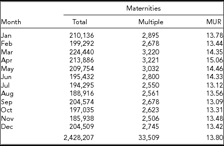
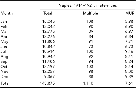
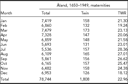
The data considered in this study are presented in the appendix and comprise the following: Neefe's Danish data in Table A1, Weinberg's data from Denmark in Table A2 and from Switzerland in Table A3, Cristalli's data from Naples (Italy) in Table A4, and Eriksson's twinning data from the Åland Islands (Finland) in Table A5. In all datasets, with the exception of Eriksson (1973), the authors consider multiple maternities instead of twin maternities. Table A3 differs from the others because the data are means for a 15-year period. In our tables, we have included the rates of multiple maternities (MURs).

Chi-Squared Tests

Fellman and Eriksson (2009) tested the seasonality of births and deaths by chi-squared tests. Let N_i be the observed number of births in month number i and let k_i be the length of the month in days. Furthermore, let N = ∑¹² _{i = 1} N_i be the total number of births and let k = ∑¹² _{i = 1} k_i be the length of the year. The expected number of births in month number i is ${\hat{N}_i} = {k_i}\frac{N}{k}$ . The chi-squared test is

(1) $$\begin{equation} {\chi ^2} = \sum\limits_{i = 1}^{12} {\frac{{{{({N_i} - {{\hat{N}}_i})}^2}}}{{{{\hat{N}}_i}}}} \end{equation}$$

with 11 degrees of freedom. Obviously, a similar test holds for deaths.

For twin and other multiple maternities, we have to modify the test. Let n_i be the number of twin maternities in month number i and let n be the total number of twin maternities. The mean twinning rate (TWR) is $r = \frac{n}{N}$ and the expected number of twin maternities in month number i is ${\hat{n}_i} = r{N_i}$ . Hence, the chi-squared test is

(2) $$\begin{equation} {\chi ^2} = \sum\limits_{i = 1}^{12} {\frac{{{{({n_i} - {{\hat{n}}_i})}^2}}}{{{{\hat{n}}_i}}}} \end{equation}$$

with 11 degrees of freedom.

The critical values for chi-squared tests with 11 degrees of freedom are χ ² = 19.68 for p < .05, χ ² = 24.73 for p < .01, and χ ² = 31.26 for p < .001.

Sinusoidal Model Building

St. Leger (1976) assumed that the pattern of the seasonal variation is sine-shaped, and he estimated the sine curve by a maximum likelihood approach. Fellman and Eriksson (1999a) considered a regression approach, and this will be used in this study. Consider the sinusoidal model

(3) $$\begin{equation} E({Y_i}) = C + A\sin ({t_i} + \alpha). \end{equation}$$

The equation can be written as

(4) $$\begin{eqnarray} E({Y_i}) &=& C + A\sin ({t_i} + \alpha) \nonumber\\ &=& C + A\cos ({t_i})\sin (\alpha) + A\sin ({t_i})\cos (\alpha) \nonumber\\ &=& \;C + {B_1}\cos ({t_i}) + {B_2}\sin ({t_i}), \end{eqnarray}$$

where Y_i is the observed rate for month number i, and t_i is an angle created from the time (in months) and B₁ = Asin(α) and B₂ = Acos(α).

The parameter estimation is based on the simplified model:

(5) $$\begin{equation} Y = A + {B_1}\cos ({t_i}) + {B_2}\sin ({t_i}) \end{equation}$$

The intercept and the parameters B ₁ and B ₂ are estimated by ordinary least squares (OLS) for the monthly data, and the initial parameters can be calculated by the equations

(6) $$\begin{equation} \hat{A} = \sqrt {\hat{B}_1^2 + \hat{B}_2^2} \end{equation}$$

and

(7) $$\begin{equation} \tan (\hat{\alpha }) = \frac{{{{\hat{B}}_1}}}{{{{\hat{B}}_2}}}. \end{equation}$$

Fellman and Eriksson (2002) presented without argumentations or proofs that ${\rm{Var}}(\hat{A}) \approx {\rm{Var}}({\hat{B}_1}) \approx {\rm{Var}}({\hat{B}_2})$ .

This assumption underestimates ${\rm{Var}}(\hat{A})$ and overestimates the significance of the sinusoidal model. In the following, we try to improve the valuation of the ${SE}_{\hat{A}}$ .

$$\begin{eqnarray*} {\rm{Var}}(\hat{A}) &=& E({\hat{A}^2}) - {\left({E(\hat{A})} \right)^2} = E\left({\hat{B}_1^2 + \hat{B}_2^2} \right) - {\left({E(\hat{A})} \right)^2}\\ &=& {\rm{Var}}({\hat{B}_1}) + {\left({E({{\hat{B}}_1})} \right)^2} + {\rm{Var}}({\hat{B}_2})\\ &&\quad +\, {\left({E({{\hat{B}}_2})} \right)^2} - {\left({E(\hat{A})} \right)^2} \\ &\approx & {\rm{Var}}({\hat{B}_1}) + \hat{B}_1^2 + {\rm{Var}}({\hat{B}_2}) + \hat{B}_2^2 - {\left({E(\hat{A})} \right)^2} \\ &\approx & {\rm{Var}}({\hat{B}_1}) + {\rm{Var}}({\hat{B}_2}) + {\hat{A}^2} - {\left({E(\hat{A})} \right)^2}\\ &\approx & {\rm{Var}}({\hat{B}_1}) + {\rm{Var}}({\hat{B}_2}). \end{eqnarray*}$$

Hence,

(8) $$\begin{equation} S{E_{{{\hat{A}}^2}}} \approx \sqrt {{\rm{Var}}({{\hat{B}}_1}) + {\rm{Var}}({{\hat{B}}_2})}. \end{equation}$$

On account of the fact that the angle α and the amplitude A have to be estimated from formulae (6) and (7), statistically non-significant estimates ${\hat{B}_1}$ and ${\hat{B}_2}$ cannot be ignored. Therefore, Fellman and Eriksson (2002) recommended full pairs of trigonometric terms. Another argument for this is that $\hat{A}$ may differ significantly from zero, but the angle $\hat{\alpha }$ may be such that ${\hat{B}_1}$ or ${\hat{B}_2}$ is close to zero and consequently assumed non-significant. The geometric interpretation is that when one fits the model to the data one focuses on the initial model in (2), and consequently, the amplitude A and the angle α are of interest. From this, it follows that the parameter tests for significance should be applied to ${\hat{A}}$ and ${\hat{\alpha}}$ , but not to ${\hat{B}_1}$ or ${\hat{B}_2}$ . These assumptions indicate that the intercept C is an estimate of the mean annual level of the rate of multiple maternities. The association between the intercept C and the total MUR can be seen later in Table 2. The amplitude A can be used as a measure of the seasonality (the model varies between C + A and C − A). Finally, the adjusted coefficient of determination, ${\bar{R}^2}$ , is a measure of the goodness of fit, and one has to pay special attention to how well the model fits the data. If the goodness of fit is poor, the non-significant results obtained can erroneously lead to the statement that the seasonality is slight, although the observed seasonal fluctuations are marked. Fellman and Eriksson (2002) noted this discrepancy and suggested the use of more general trigonometric regression models. In this study, we consider only sinusoidal models and use the adjusted coefficient of determination, ${\bar{R}^2}$ , as a measure of the goodness of fit. In Table 1, the estimates are included for all datasets. The significance of the model can also be checked by comparing ${\hat{A}}$ , which is always positive, and $S{E_{\hat{A}}}$ . Although ${\hat{A}}$ is by no means normally distributed, it can be considered approximately normal and $t = \frac{{\hat{A} - 0}}{{S{E_{\hat{A}}}}}$ should be greater than two in order that a significant deviation from zero can be considered.

TABLE 1 Collection of Chi-Squared, Standard Deviations (SDs) Measuring the Strength of Seasonality and the Adjusted Coefficient of Determination ${\bar{R}^2}$ Measuring the Goodness of Fit for Sinusoidal Models for the MURs for Different Datasets

Goodness of fit for the Danish legitimate dataset is (0.672), the Åland dataset is (0.630), the dataset for Denmark is (1855–1894) (0.577), and the total Danish dataset is (1855–1869) (0.535). The estimates for the Switzerland data are based on 15 annual means and are not comparable to the other estimates. This is discussed in the text. For the rest of the data, the adjusted coefficients of determination ${\bar{R}^2}$ are below 0.500, which we consider the limit for an acceptable strength of seasonality.

Results

In Table A1, we present the Danish data according to Neefe (1877). We follow Neefe and present his data for rural and urban, legitimate and illegitimate, and total data. In the table, we have included all maternities, multiple maternities, and the monthly rates of multiple maternities (MURs). In Figure 1a, we present the MURs of the subsets for urban and rural data and in Figure 1b the subsets for legitimate and illegitimate data. The figures also include the total dataset and the seasonal models. The figures indicate that the seasonality is strongest for the illegitimate data, followed by the urban data. For the other datasets, the seasonality is rather similar. These findings are supported by the standard deviations given in Table 1. Also included in Table 1 are chi-squared tests for the strength of the seasonality. The obtained chi-squared test results indicate that seasonality is significant for all datasets. In Figure 1a and b, we have included the sinusoidal models for the datasets. The inclusion of these models describes the general seasonal pattern of these datasets. The obtained models are discussed below.

FIGURE 1 Comparison between the MURs for the total dataset, the urban and rural subdata (a) and the legitimate and illegitimate subdata (b) in Denmark in 1855–1869 (Neefe, 1877). The corresponding sinusoidal models are included.

Weinberg's Danish data for the total and multiple maternities are presented in Table A2 and his data for Switzerland in Table A3 (Weinberg, 1901). In Table A4, we present the data for Naples according to Cristalli (1924). In fact, we identified a misprint in Cristalli's tables. This misprint is corrected in our analyses. In Figure 2, we include the data from Switzerland (1876–1890) and Naples (1914–1921). According to the chi-squared test results in Table 1, the Naples data show slight significant seasonality. The Switzerland data are means of 15 annual data, and therefore the chi-squared value should be multiplied by 15 in order to yield a value comparable with the Naples test result (15 × 2.74 = 41.1). Later, when we consider sinusoidal models, we return to the means of 15 annual data for Switzerland. The seasonality for Denmark for both the Neefe and Weinberg data is marked. Eriksson's data of twin maternities from the Åland Islands (Finland) are presented in Table A5. According to Table 1, the seasonality for Åland is remarkably strong. The analyses of the sinusoidal models are presented below.

FIGURE 2 Comparison between the MURs for Switzerland, 1876–1890 (Weinberg, 1901) and Naples, 1914–1921 (Cristalli, 1924). The corresponding sinusoidal models are included.

Sinusoidal Model Building

We built sinusoidal models for all datasets. Below, we analyze the results using the goodness of fit measured with the adjusted coefficient of determination. The Switzerland data result in a model that has the best goodness of fit. The model is

$$\begin{eqnarray*} Y = 12.391 - 0.247\,\cos ({t_i}) + 0.779\,\sin ({t_i}). \end{eqnarray*}$$

Hence, $SE({\hat{B}_1}) = 0.112$ , $SE({\hat{B}_2}) = 0.112$ , and ${\bar{R}^2} = 0.824$ . The first parameter is almost significant and the second is significant. The obtained estimates of the initial parameters are $\hat{A} = 0.818$ and $\hat{\alpha } = - 17.6^\circ$ . When we use ${\bar{R}^2}$ as a measure of significance, the Switzerland data give the best goodness of fit and the model is acceptable. However, the obtained value $\hat{A} = 0.818$ indicates that the seasonality is weak.

The obtained results for Åland are

$$\begin{eqnarray*} Y = 23.207545 - 2.457893\,\cos ({t_i}) - 2.737970\,\sin ({t_i}). \end{eqnarray*}$$

where

$$\begin{eqnarray*} {\rm{Var}}({\hat{B}_1}) = 0.811,\;{\rm{Var}}({\hat{B}_2}) = 0.809\;{\rm{and}}\;{\bar{R}^2} = 0.630 \end{eqnarray*}$$

Both parameter estimates are significant. The obtained estimates of the initial parameters are $\hat{A} = {\rm{3}}{\rm{.679}}$ and $\hat{\alpha } = {\rm{221}}{\rm{.9}}^\circ$ . According to the ${\hat{A}}$ value, the seasonality is strong; in fact, the strongest among all datasets. The seasonality of the Åland data is given in Figure 3.

FIGURE 3 Comparison between twinning rates for Åland, 1750–1949 (Eriksson, 1973), and multiple maternity for Denmark, 1855–1894 (Weinberg, 1901) and Naples (Italy), 1914–1920 (Cristalli, 1924). The sinusoidal models are illustrated with dashed lines. For details, see the text.

For Denmark (1855–1894), the obtained results are

$$\begin{eqnarray*} Y = 13.780202 - 0.182516\,\cos ({t_i}) + 0.653557\,\sin ({t_i}), \end{eqnarray*}$$

where ${\rm{Var}}({\hat{B}_1})\! =\! 0.164639$ , ${\rm{Var}}({\hat{B}_2}) \!=\! 0.164295$ , $\hat{A} \!=\! 0.678564$ , $\hat{\alpha } = - 15.6^\circ$ and ${\bar{R}^2} = 0.577$ . Only the second parameter estimate is significant, but as pointed out above, both terms should be included in the model. Furthermore, the Neefe data for urban, legitimate, and total data in Denmark (1855–1869) yields acceptable goodness of fit. The obtained model for Denmark is

$$\begin{eqnarray*} Y = 14.489480 - 0.086058\cos (t) + 0.893885\,\sin (t), \end{eqnarray*}$$

where ${\rm{Var}}({\hat{B}_1}) = 0.234818$ , ${\rm{Var}}({\hat{B}_2}) = {\rm{0}}{\rm{.234327}}$ , $\hat{A} = 0.898$ , $\hat{\alpha } = - 5.5^\circ$ , and the adjusted coefficient of determination, ${\bar{R}^2} = 0.535.$

For the rest of the datasets, the model-building results yield low adjusted coefficients of determination ( ${\bar{R}^2} < 0.500$ ), and we assume that the goodness of fit is so slight that the corresponding models should not be discussed. The estimates of the parameters and their standard errors (SEs) for all datasets are given in Table 2.

TABLE 2 Test Results of the Sinusoidal Models

The population data resulting in R ² > 0.500 are discussed in the text. The rate of MUR is the overall rate of multiple maternities, and the association between MUR and the intercept C can be analyzed in the table (the α is about 30° per month).

^a The negative value is a consequence of a very bad fit with too many regressors.

Considering the periods 1855–1869 and 1870–1894, we can compare the temporal changes in the MURs for Denmark. In Figure 4, one can observe similar seasonal models for the MURs, but also a decrease on average of about 1.08 per 1,000. In Figure 3, we present the Åland data, the Weinberg dataset for Denmark (1855–1894), and the Naples data relative to the corresponding sinusoidal models. The variable seasonality strength is apparent.

FIGURE 4 Comparison in seasonality in Denmark in 1855–1869 and 1870–1894. The corresponding sinusoidal models are included.

Discussion

Fellman and Eriksson (1999b) used Walter and Elwood's (1975) sinusoidal model to evaluate the seasonal variation in the twinning rate in Denmark, Switzerland, England, and Wales. Fellman and Eriksson (1999b) studied the secular changes in the seasonal patterns of births in Sweden, Norway, and Iceland. They introduced a modified Walter–Elwood model and investigated the temporal variations in the Walter–Elwood theta and quarters with high and low numbers of births per day. Fellman and Eriksson (2002) studied the temporal changes in births and death using trigonometric regression models. The trigonometric regression models are generalizations of the sinusoidal model. They are used when the general pattern of the graphs is too complicated for a sinusoidal model. That study was based on data from Italy, France, Germany, Denmark, Norway, Scotland, Sweden, and Iceland. Special attention was paid to data from Iceland. Eriksson et al. (2008) considered the seasonality in births and deaths on the Åland Islands. Finally, Fellman and Eriksson (2009) considered births for the Åland Islands and its sub-regions and introduced a new measure of the strength of the seasonality.

Conclusions

When seasonality is studied, one must decide whether one seeks the strength of the seasonality or whether one seeks a seasonality model. When seasonal models are applied, one pays special attention to how well the model fits the data. In this study, we used the test of the amplitude $\hat{A}$ and the adjusted coefficient of determination ${\bar{R}^2}$ as measures of goodness of fit (cf. Table 2). If goodness of fit is poor, the non-significant results obtained can erroneously lead to a statement that the seasonality is slight, although the observed seasonal fluctuations are marked (cf. Switzerland and Naples). Under such circumstances, the use of more general trigonometric regression models could be considered.