


1. Introduction
Narrow bracketing receives growing attention in behavioral economics. It highlights the fact that individuals tend to be myopic in specific investment decisions, consequently overlooking the comprehensive portfolio, which, strictly speaking, should encompass non-financial wealth such as human capital. People affected by the tendency to narrowly bracket decisions would not be able to take full advantage of hedging, which requires a joint evaluation of risky prospects.Footnote 1 There is a diverse and growing literature showing the importance of narrow bracketing in explaining choices under uncertainty that are otherwise inconsistent with standard economic theories. Examples include the equity premium puzzle (Barberis et al., Reference Barberis, Huang and Santos2001, Barberis & Huang, Reference Barberis, Huang and Mehra2006, Mehra & Prescott, Reference Mehra and Prescott1985), non participation in stock markets (Barberis et al., Reference Barberis, Huang and Thaler2006), and the observed underinsurance in various insurance markets (Gottlieb, Reference Gottlieb2012, Gottlieb & Smetters, Reference Gottlieb and Smetters2021, Zheng, Reference Zheng2020).Footnote 2 An important feature of narrow bracketing that has been taken for granted in theoretical models is that individuals can be partially narrow bracketing in the sense that their behavior lies between fully myopic and fully broad bracketing.
So far, however, empirical research on narrow bracketing is limited to demonstrating the relevance of narrow bracketing (Gottlieb & Mitchell, Reference Gottlieb and Mitchell2020, Rabin & Weizsäcker, Reference Rabin and Weizsäcker2009, Tversky & Kahneman, Reference Tversky and Kahneman1981), and the existence and property of partial narrow bracketing has received little attention.Footnote 3 It is critical to understand the heterogeneity in narrow bracketing among individuals as we need this information to guide empirical studies and policies aiming to counteract narrow bracketing. On the one hand, the extreme choices driven by unobserved heterogeneity can bias group estimates of narrow bracketing without bounded constraints of narrow bracketing. On the other hand, if bounded constraints are imposed while neglecting intermediate types, we may still overestimate the degree of narrow bracketing by attributing intermediate types to complete narrow bracketing. Thus, we investigate the distribution of narrow bracketing in our sample by estimating the individual degree of narrow bracketing. We contribute to the literature by quantitatively uncovering the heterogeneity with rich observations per subject and a well-founded behavioral model.
Specifically, we design a lab experiment to investigate narrow bracketing in the context of investment and insurance decisions.Footnote 4 To test the underlying behavioral model, we adopt three features in the experiment. First, each subject was asked to respond to two types of experimental tasks: an investment task (task INV) and an insurance task (task INS). As illustrated in our upcoming example, task INS serves as the experimental treatment that adds preexisting risks to the same decisions as in task INV, turning risky lotteries into full insurance against preexisting risks for subjects without narrow bracketing. Second, in each task, we elicit subjects’ willingness to pay (WTP) for a common set of lotteries using lists of prices , which gives us information on subjects’ preferences in rich situations. Third, inspired by prospect theory (Kahneman & Tversky, Reference Kahneman and Tversky1979), we introduce preexisting risks in both gain and loss domains to have a comprehensive understanding of the impact of narrow bracketing on hedging. The insurance task includes two subtasks: task INS-G in the gain domain and task INS-L in the loss domain.
Consider the following example involving a lottery that generates a payoff of € 10 with a 50% chance. The initial endowment is € 10 for all the subjects. In task INV, subjects were asked to decide whether to buy the lottery against a price list ranging from € 0 to € 10 with a gap of .5. In task INS-G (or INS-L), subjects were asked to assess the lottery against the same price list given a pre existing risk – the uncertainty of winning € 10 (or losing € 10) that is perfectly negatively correlated with the lottery. Essentially, purchasing the lottery in the insurance tasks is equivalent to buying full insurance against preexisting risks, that is, a sure € 10 gain in task INS-G and a sure € 0 loss in task INS-L. In each task, subjects were asked to respond to four lotteries with different chances and price ranges; in total, 12 lotteries. We compare individual risk-taking behaviors within and between subjects while manipulating the risks they face ex ante.
Before proceeding to our theoretical predictions under narrow bracketing, let us start with the theory without narrow bracketing. According to expected utility theory, more risk-averse subjects should have a lower WTP for lotteries in task INV but a higher WTP in tasks INS-G and INS-L, generating a negative correlation between the two WTPs.Footnote 5 Assuming risk aversion, we anticipate the elicited WTP to be lower than the expected values of the lotteries in task INV and higher in tasks INS-G and INS-L. In the case of constant relative risk aversion (CRRA) utility, the WTP in task INS-L should be higher than in task INS-G.
Now, we delve into the predictions considering narrow bracketing. Our model combines prospect theory (Kahneman & Tversky, Reference Kahneman and Tversky1979) and narrow bracketing (Rabin & Weizsäcker, Reference Rabin and Weizsäcker2009). Let us begin by considering two extremes: completely broad bracketing and completely narrow bracketing. In the former case, we align with the predictions of prospect theory (Kahneman & Tversky, Reference Kahneman and Tversky1979), characterized by an S-shaped utility curve with a kink at the reference point, symbolizing loss aversion. Consequently, our predictions are as follows: The WTP for lotteries in task INV should be lower than their expected values due to the influence of loss aversion on individual risk attitudes in low-stake decisions, inducing first-order risk aversion (Rabin, Reference Rabin2000).Footnote 6 Under weak concavity, the WTP in task INS-G is expected to be slightly higher than the expected values of the lotteries and slightly lower than those in task INS-L. In the other extreme case, completely narrow bracketers would ignore preexisting risks while evaluating lotteries, neglecting the opportunity of hedging. Consequently, lotteries will have the same valuations across different tasks. For more general cases involving partial narrow bracketing, we anticipate the following: the more risk-averse (or loss-averse) individuals behave in the investment task, the less they are willing to pay for insurance in the insurance tasks. To be more explicit, this positive correlation arises through a positive degree of narrow bracketing. When insurance is narrowly perceived as a gamble (see, e.g.,Giesbert et al., Reference Giesbert, Steiner and Bendig2011, Kahneman & Lovallo, Reference Kahneman and Lovallo1993, Kahneman, Reference Kahneman2003), more risk-averse individuals will find it less attractive, ceteris paribus.
In line with the predictions, we find that participants who were less willing to take risks in the investment task also spent less on insurance. We further confirm this result by employing a qualitative, validated, survey-based measure of individual willingness to take risks “in general,” which has been shown to yield accurate predictions for various real-life risky situations (Dohmen et al., Reference Dohmen, Falk, Huffman, Sunde, Schupp and Wagner2011). These results are consistent with the findings of several recent studies that specifically investigate the impact of loss aversion on insurance behaviors using US data (Hwang, Reference Hwang2021, Gottlieb & Mitchell, Reference Gottlieb and Mitchell2020) and European data (Eling et al., Reference Eling, Ghavibazoo and Hanewald2021). Our experimental tasks in the gain domain also replicate the main results of Frederick et al. Reference Frederick, Meyer and Levis2015, and Frederick et al. Reference Frederick, Levis, Malliaris and Meyer(2018), which used 50-50 lotteries paying out $10, showing that subjects do not sufficiently value hedges and that there is a positive correlation between valuations of hedges and bets. In addition, we find that participants in the insurance task hedged significantly more in the gain domain than in the loss domain. Taken together, our experimental results can be explained by combining prospect theory and a positive degree of narrow bracketing.
Correspondingly, we estimate a structural model embedding three features: prospect theory, domain-specific hedging behavior, and an individual-specific degree of narrow bracketing. We avoid restricting any correlation between individual narrow bracketing and individual characteristics. It turns out that extreme and intermediate types constitute a substantial share of subjects. Thus, the extreme-type assumption in Rabin Reference Rabin(2000) and the assumption of partial narrow bracketing in theoretical works fit part of the reality. We further demonstrate the potential issue of overestimating the degree of narrow bracketing, which may happen if we neglect the existence of partial narrow bracketing or the bounded nature of narrow bracketing. As a result, researchers may also misinterpret the relationship between narrow bracketing and individual characteristics. We find that the relation between gender/numeracy ability (Skagerlund et al., Reference Skagerlund, Lind, Strömbäck, Tinghög and Västfjäll2018) and narrow bracketing is smaller than that derived from group estimates. In addition, the estimated relation with cognitive ability goes in opposite directions between our model and that directly estimating group-average degree of narrow bracketing. Recent work by Koch and Nafziger Reference Koch and Nafziger(2019) examined the mechanism driving narrow bracketing – whether it stems from choice errors due to cognitive limitations or strategic efforts for self-control. The study revealed more consistent evidence supporting the self-control mechanism, with less consistent findings for cognitive limitations. In this important debate, the direction of estimated relations is crucial.
This paper contributes to four branches of the literature. First, it adds to the extensive literature on narrow bracketing in two main aspects.Footnote 7 Dating back to Tversky and Kahneman Reference Tversky and Kahneman1981 and more recently, Rabin and Weizsäcker Reference Rabin and Weizsäcker(2009), researchers conducted lab experiments and demonstrated the existence of narrow bracketing using dominated choices.Footnote 8 With cleverly designed tasks, a subject who succumbs to narrow bracketing and makes each decision in isolation from the rest can violate stochastic dominance and lose a certain amount of money. Our contribution lies in empirically demonstrating the relevance of partial narrow bracketing in decision-making. Additionally, we explore individual heterogeneity in narrow bracketing, which can have important implications for policies, like the obstacles of screening different types of individuals and correcting the effect of narrow bracketing. While several attempts in the literature have addressed this aspect, they face challenges in estimating the individual degree of partial narrow bracketing due to constraints in their experimental settings. For instance, Guiso Reference Guiso(2015) considered partial narrow bracketing and examined respondents’ decisions in entering a small and hypothetical lottery of winning € 180 with the probability of 1/2 or losing € 100 with the same probability while manipulating their accessibility to their labor income risks. However, due to a lack of observations at the individual level, he provided a range for individual degrees of narrow bracketing by making certain assumptions about utility functions. In a recent study, Ellis and Freeman Reference Ellis and Freeman(forthcoming) adopted a revealed preferences approach to study narrow bracketing. They could test for broad or narrow bracketing by checking the rationalization of their data, but the study remained silent about the precise degree of narrow bracketing. We further discuss the resulting estimation bias, which is relevant to all empirical studies of narrow bracketing that are interested in quantifying the effect of narrow bracketing.
This paper also contributes to the literature on risk-taking and narrow bracketing by estimating the individual-level effect of narrow bracketing on hedging. A growing literature looks at how various types of behavioral bias affect hedging decisions (Pitthan & De Witte, Reference Pitthan and De Witte2021). Most of these studies have taken the form of surveys. For instance, Brown et al. Reference Brown, Kling, Mullainathan and Wrobel(2008) found that an annuity was much more likely to be chosen by their respondents when the annuity payment and the other income were aggregated in terms of consumption than when described in terms of annuity payments in isolation.Footnote 9 As previously mentioned, Guiso Reference Guiso(2015) tested narrow bracketing by manipulating how cognitively accessible their labor income risks were and found that individuals who were induced to bring their earnings risk to mind were significantly less likely to turn down the lottery. Gottlieb and Mitchell Reference Gottlieb and Mitchell(2020) found that respondents subject to narrow bracketing were less likely to purchase long-term care insurance. Respondents were asked two hypothetical questions in a public policy context, based on the classic experiments from Tversky and Kahneman Reference Tversky and Kahneman1981. The questions were qualitatively the same but presented in either a gain or loss framing. If respondents’ answers differed between these two questions, they were classified as narrow bracketers. While showing that narrow bracketing makes insurance unattractive, they are all silent on precise preferences and the magnitude of individual-level effects, partly due to the lack of observations per respondent.
Thirdly, this paper contributes to the recent literature examining the relationship between betting and hedging behaviors. In a similar setting as in our investment task and insurance task in the gain domain, recent studies by Frederick et al. Reference Frederick, Meyer and Levis2015, Frederick et al. Reference Frederick, Levis, Malliaris and Meyer(2018), and Chatterjee and Mookherjee Reference Chatterjee and Mookherjee(2018) also find a positive correlation between valuations of a bet and its perfect hedge, and the undervaluation of hedges. As Frederick et al. Reference Frederick, Levis, Malliaris and Meyer(2018) wrote, “Respondents clearly fail to appreciate the covariance between bets and hedges fully; the pattern remains distinct from complete covariance neglect, in which hedges and bets are treated as independent.” This is reminiscent of partial narrow bracketing as posed in our study. It is, however, worth stressing that our experimental design was mainly theory-driven, especially based on the theory of narrow bracketing as initially proposed by Rabin and Weizsäcker Reference Rabin and Weizsäcker(2009), and introduced varying preexisting risks as experimental treatments. We have also provided sound theoretical predictions, which are directly testable. Moreover, we included insurance tasks in the loss domain, allowing us to have a complete picture of decision-making and to estimate preferences of a prospect-theory type. Our structural estimation pinpoints the relevance of narrow bracketing in hedging decisions at the individual level. Furthermore, these studies have shown that many popular decision theories under risk fail to explain their results, particularly the positive correlation between bets and hedges, which they described as “difficult to expunge,” as noted in the abstract of Frederick et al. Reference Frederick, Meyer and Levis2015.Footnote 10 We show that the seemingly puzzling results could be reconciled with the theory of narrow bracketing. Interestingly, Newall and Cortis Reference Newall and Cortis(2019) find that the same phenomena observed in previous lab experiments were also evident for high-stakes hedges in the field using the 2015/16 English Premier League. The robust and consistent findings in the literature further underscore the significance of narrow bracketing in decision-making.
Lastly, our paper contributes to a broad literature on how people manage, hedge, and mitigate the risks they face. In particular, behavioral biases often hinder efficient risk management. For example, Markle and Rottenstreich Reference Markle and Rottenstreich(2018) find that an unresolved “background” position, to which people are already exposed, can influence their risk attitudes toward new “focal” prospects due to their preferences for consistency. Lewis and Simmons Reference Lewis and Simmons(2020) document that people tend to incur high costs to improve the likelihood of favorable outcomes, even when those outcomes are already quite likely. Similarly, Ryan et al. Reference Ryan, Baum and Evers(2024) find that individuals assess the relative reduction in negative outcomes differently depending on their initial chances of success. Lewis et al. Reference Lewis, Feiler and Adner(2023) demonstrate that when managing multiple risks simultaneously – where one risk is less likely than the other but both are necessary for overall success – people often employ the worst-first heuristic and invest more to improve the chances of less likely requirements rather than more likely ones, even when the latter improvements would have an equally significant impact on overall success. Our paper complements this literature by highlighting that narrow bracketing could present another significant “obstacle” to achieving efficient risk management.
The remainder of this paper is organized as follows. Section 2 describes the theory of narrow bracketing and its predictions in an experiment tailored for testing it. Section 3.1 explains the experimental design and procedures. Section 4 presents our results on theory testing, and Section 5 structurally estimates individual preferences and the degree of narrow bracketing. Section 6 concludes.
2. Theory of narrow bracketing and its predictions
In this section, we derive theoretical predictions of narrow bracketing in hedging decisions. Section 2.1 presents the theory of narrow bracketing first introduced by Rabin and Weizsäcker Reference Rabin and Weizsäcker(2009). In the model, the decision maker’s preference is described jointly by prospect theory and a positive degree of narrow bracketing. Section 2.2 derives the prediction of narrow bracketing in two types of tasks: an investment task and insurance tasks in the gain domain and the loss domain.
2.1. Setup
Utility preferences Following Rabin and Weizsäcker Reference Rabin and Weizsäcker(2009), we assume that the objective function of a decision maker (she) is given byFootnote 11
 \begin{equation}
\max_{\tilde{x} \in \mathcal{X}}EV(\tilde{x}+\tilde{y}, \tilde{x})=(1-k)Eu(\tilde{x}+\tilde{y})+kEg(\tilde{x}),
\end{equation}
\begin{equation}
\max_{\tilde{x} \in \mathcal{X}}EV(\tilde{x}+\tilde{y}, \tilde{x})=(1-k)Eu(\tilde{x}+\tilde{y})+kEg(\tilde{x}),
\end{equation} where  $\tilde{x}$ represents the acquired risk from a choice set
  $\mathcal{X}$ and
  $\tilde{y}$ represents the preexisting risk.
  $k\in[0,1]$ is the degree of narrow bracketing: when k = 1, the decision maker is a fully narrow bracketer who evaluates the newly acquired risk
  $\tilde{x}$ in isolation; when k = 0, she is a fully broad bracketer who evaluates the new risk together with the preexisting risk
  $\tilde{y}$; otherwise, she is a partially narrow bracketer who does both. That is to say, the prediction of a model without narrow bracketing is the same as having k = 0. Following Kahneman and Tversky Reference Kahneman and Tversky(1979), we assume that the utility functions
  $u(\cdot)$ and
  $g(\cdot)$ take the following form:
 \begin{equation}
u(x)=g(x)=
\begin{cases}
v(x),& \text{if}\ x \geq 0; \\
-\lambda v(-x), & \text{otherwise.}
\end{cases}
\end{equation}
\begin{equation}
u(x)=g(x)=
\begin{cases}
v(x),& \text{if}\ x \geq 0; \\
-\lambda v(-x), & \text{otherwise.}
\end{cases}
\end{equation} λ > 1 measures the degree of loss aversion. The value function  $v(\cdot)$, which applies to changes in wealth relative to the reference point (normalized to zero), is assumed to be increasing and concave. Assuming the same functional form for u(x) and g(x) directly implies that if there is no risk ex-ante (that is,
  $\tilde{y}=0$), narrow bracketing will not affect risk-taking at all (see Equation (2.1)). The S-shaped utility function captures the reflection effect observed in many lab experiments; namely, the decision-maker is risk-averse in the gain domain and risk-seeking in the loss domain. The strong domain-specific risk behavior in the data further supports the assumption made here. For ease of presentation, we abstract from probability weighting in prospect theory and derive theoretical predictions without it. This simplification does not impact the hypothesis testing narrow bracketing.Footnote 12
Risk We use two-outcome lotteries, that is, win  $\overline{x}$ when event E with known probability p is realized and
  $\underline{x}\leq \overline{x}$ otherwise. The notation
  $\overline{x}_{E}\underline{x}$ is hereafter a shorthand for
  $(E:\overline{x};\ E^{c}:\underline{x})$. Let µ denote the mean of the lottery, that is,
  $\mu=p\overline{x}+(1-p)\underline{x}$. We also assume that subjects who broadly bracket take the initial endowment as their reference point, and those who narrowly bracket consider the initial endowment plus the preexisting risk as their reference point. Note that this is a common assumption in the literature. Existing experimental studies also provided empirical support. For instance, Baillon et al. Reference Baillon, Bleichrodt and Spinu(2020) found evidence for subjects taking the status quo as their reference point. Etchart-Vincent and L’Haridon Reference Etchart-Vincent and L’Haridon(2011) found that subjects’ behaviors were similar in the face of losses from an initial endowment and those coming out of their own pockets.
Tasks As narrow bracketing affects decision-making only when there is a preexisting risk, we derive behavioral predictions of narrow bracketing in two types of tasks: investment task (task INV, without preexisting risk) and insurance task (task INS, full insurance against preexisting risk). The insurance task includes two scenarios, as individuals are expected to behave differently depending on whether preexisting risks happen in the gain or loss domain. The task in the gain domain (i.e., INS-G) has all outcomes of preexisting risks non-negative, while the task in the loss domain (i.e., INS-L) has all the outcomes of preexisting risks non-positive. Specifically, for a broad bracketer, acquiring a lottery means a  $(\overline{x}+\underline{x})$ gain regardless of lottery realization in task INS-G and zero loss in task INS-L, no matter of event E or Ec. For a complete narrow bracketer, acquiring a lottery in the task INS-G and INS-L is the same as that in the task INV.
Comparing individual insurance behaviors in tasks INS-G and INS-L can let us test the S-shaped utility functions advocated in prospect theory. This can further help rule out other alternative decision theories as possible explanations for our data.
2.2. Prediction of narrow bracketing
Our theoretical predictions center on the interplay between willingness to pay for the same lottery across different experimental tasks. Under many decision theories such as expected utility, rank-dependent expected utility (Quiggin, Reference Quiggin1982), regret (e.g., Loomes & Sugden, Reference Loomes and Sugden1982, Bell, Reference Bell1982) and disappointment theory (e.g., Gul, Reference Gul1991), investment and insurance behaviors are just two sides of the same coin in these decision models. We provide an in-depth analysis of willingness to pay under these theories in the online appendix. Notably, all these theories predict a negative correlation between the valuations of lotteries when they are considered investments and when they are considered full insurance. However, recent experimental and field studies (e.g., Eling et al., Reference Eling, Ghavibazoo and Hanewald2021, Frederick et al., Reference Frederick, Meyer and Levis2015, Frederick et al., Reference Frederick, Levis, Malliaris and Meyer2018) point to the opposite direction, though they do not connect their findings to narrow bracketing. As we will elucidate further, the combined theory of narrow bracketing and prospect theory produces predictions in line with positive correlations. These unique forecasts enable us to differentiate narrow bracketing from alternative explanations.
2.2.1. Investment task – INV
In task INV, buying a lottery  $\overline{x}_{E}\underline{x}$ with
  $0 \leq \underline{x}\leq \overline{x}$ at a price between
  $\overline{x}$ and
  $\underline{x}$ realizes a gain when the high outcome occurs but a loss when the low outcome occurs. The agent’s willingness to pay for such a lottery, denoted as WTPV, is the value such that
 \begin{equation}
pv(\overline{x}-WTP_{V})-\lambda (1-p)v(WTP_{V}-\underline{x})=0.
\end{equation}
\begin{equation}
pv(\overline{x}-WTP_{V})-\lambda (1-p)v(WTP_{V}-\underline{x})=0.
\end{equation}By fully differentiating Equation (2.3) with respect to λ, we obtain
 \begin{equation*}
\frac{\partial WTP_{V}}{\partial \lambda}=-\frac{(1-p)v(WTP_{V}-\underline{x})}{pv'(\overline{x}-WTP_{V})+\lambda(1-p)v'(WTP_{V}-\underline{x})} \lt 0.
\end{equation*}
\begin{equation*}
\frac{\partial WTP_{V}}{\partial \lambda}=-\frac{(1-p)v(WTP_{V}-\underline{x})}{pv'(\overline{x}-WTP_{V})+\lambda(1-p)v'(WTP_{V}-\underline{x})} \lt 0.
\end{equation*}Intuitively, loss aversion implies a first-order risk aversion at the status quo. The more loss-averse the agent is, the less she is willing to take risks, hence the smaller WTPV. To characterize the size of WTPV, we can rewrite Equation (2.3) in the following way:
 \begin{equation}
\lambda\frac{1-p}{p}=\frac{v(\overline{x}-WTP_{V})}{v(WTP_{V}-\underline{x})}{{\large \gt }} \frac{v(\overline{x}-\mu)}{v(\mu-\underline{x})}=\frac{v((1-p)(\overline{x}-\underline{x}))}{v(p(\overline{x}-\underline{x}))},
\end{equation}
\begin{equation}
\lambda\frac{1-p}{p}=\frac{v(\overline{x}-WTP_{V})}{v(WTP_{V}-\underline{x})}{{\large \gt }} \frac{v(\overline{x}-\mu)}{v(\mu-\underline{x})}=\frac{v((1-p)(\overline{x}-\underline{x}))}{v(p(\overline{x}-\underline{x}))},
\end{equation} where  $\mu=p\overline{x}+(1-p)\underline{x}$. Whether the above inequality holds depends on the difference between the terms on the far left and far right sides. Clearly, for p = .5, the inequality is true due to loss aversion, and this further implies that
  $WTP_{V} \lt \mu$. The inequality becomes even looser for any p < .5 because of the concavity of
  $v(\cdot)$. So
  $WTP_{V} \lt \mu$ for any
  $p\leq .5$. However, for p > .5, WTPV is smaller than µ only if
  $v(\cdot)$ is weakly concave or λ is large enough. Let us consider the following numerical example: λ = 2.25 and
  $v(x)=x^{1-\alpha}$ with α = .12. These parameter values are estimates from Tversky and Kahneman Reference Tversky and Kahneman(1992). We can show that the inequality (2.4) holds for
 \begin{equation}
p \lt \overline{p}=\frac{\lambda^{\frac{1}{\alpha}}}{1+ \lambda^{\frac{1}{\alpha}}}=0.999.
\end{equation}
\begin{equation}
p \lt \overline{p}=\frac{\lambda^{\frac{1}{\alpha}}}{1+ \lambda^{\frac{1}{\alpha}}}=0.999.
\end{equation} Replacing α, a constant relative risk aversion coefficient, by .9 (indicating extreme risk aversion in the gain domain), the threshold  $\overline{p}$ is only reduced to .71. An important message from carrying out this exercise is that the diminishing sensitivity of the value function plays a minor role in valuing lotteries in task INV. Especially for probabilities of .3, .5, or .7 that we chose in our experiment, the inequality condition is always satisfied. We summarize these results in the following proposition.
Proposition 1.
The willingness to pay for a lottery in task INV (i.e., WTPV) decreases with the degree of loss aversion λ. Furthermore, under loss aversion and weak concavity of  $v(\cdot)$, WTPV is smaller than the expected value of the lottery.
2.2.2. Treatment I: Insurance task in the gain domain – INS-G
In task INS-G, the agent faces a preexisting risk in the gain domain and has the possibility of fully insuring himself. More explicitly, the agent can buy a lottery  $\overline{x}_{E}\underline{x}$ with
  $0 \leq \underline{x}\leq \overline{x}$ to fully hedge against the preexisting risk
  $\underline{x}_{E}\overline{x}$. With probability p, the preexisting risk produces
  $\underline{x}$, and the lottery draw is
  $\overline{x}$; with probability
  $1-p$, the preexisting risk produces
  $\overline{x}$, and the lottery draw is
  $\underline{x}$. The agent’s willingness to pay for the lottery, denoted as
  $WTP^{k}_{G}$ where the superscript k indicates the degree of narrow bracketing, is the value such that
 \begin{align}
&(1-k)v(\overline{x}+\underline{x}-WTP^{k}_{G})+k[pv(\overline{x}-WTP^{k}_{G})-\lambda (1-p)v(WTP^{k}_{G}-\underline{x})] \nonumber\\
&\quad =(1-k)[pv(\underline{x})+(1-p)v(\overline{x})].
\end{align}
\begin{align}
&(1-k)v(\overline{x}+\underline{x}-WTP^{k}_{G})+k[pv(\overline{x}-WTP^{k}_{G})-\lambda (1-p)v(WTP^{k}_{G}-\underline{x})] \nonumber\\
&\quad =(1-k)[pv(\underline{x})+(1-p)v(\overline{x})].
\end{align}By fully differentiating Equation (2.6) with respect to λ, we obtain
 \begin{equation*}
\frac{\partial WTP^{k}_{G}}{\partial \lambda}=-\frac{k(1-p)v(WTP^{k}_{G}-\underline{x})}{(1-k)v'(c-WTP^{k}_{G})+k[pv'(\overline{x}-WTP^{k}_{G})+\lambda (1-p)v'(WTP^{k}_{G}-\underline{x})]} \leq 0.
\end{equation*}
\begin{equation*}
\frac{\partial WTP^{k}_{G}}{\partial \lambda}=-\frac{k(1-p)v(WTP^{k}_{G}-\underline{x})}{(1-k)v'(c-WTP^{k}_{G})+k[pv'(\overline{x}-WTP^{k}_{G})+\lambda (1-p)v'(WTP^{k}_{G}-\underline{x})]} \leq 0.
\end{equation*} Note that the above inequality is strict only for k > 0; otherwise, it is binding. Therefore, with narrow bracketing (i.e., k > 0), higher loss aversion implies lower valuations for lotteries in task INS-G when the agent has a positive degree of narrow bracketing. To characterize the size of  $WTP^{k}_{G}$, let us consider two extreme situations:
  $WTP_{G}^{0}$ and
  $WTP_{G}^{1}$. At k = 0, the agent is a fully broad bracketer, and Equation (2.6) can be rewritten as follows:
 \begin{equation*}
v(c-WTP_{G}^{0})=pv(\underline{x})+(1-p)v(\overline{x}) \lt v(c-\mu).
\end{equation*}
\begin{equation*}
v(c-WTP_{G}^{0})=pv(\underline{x})+(1-p)v(\overline{x}) \lt v(c-\mu).
\end{equation*} The last inequality is due to risk aversion in the gain domain (i.e.,  $v''(\cdot) \lt 0$). It implies that
  $WTP_{G}^{0} \gt \mu$. At k = 1, the agent fully ignores the insurance value of the lottery and views it as an independent gamble. Obviously,
  $WTP_{G}^{1}$ should be equal to WTPV. By Proposition 1, we know that
  $\mu \gt WTP_{G}^{1}$ under weak concavity of
  $v(\cdot)$. Observing that the terms on the left-hand side of Equation (2.6) are decreasing in
  $WTP^{k}_{G}$ and forming a linear combination of the two extreme cases, we have
 \begin{equation}
WTP_{G}^{0} \geq WTP^{k}_{G} \geq WTP_{G}^{1}=WTP_V, \quad \forall k\in [0,1].
\end{equation}
\begin{equation}
WTP_{G}^{0} \geq WTP^{k}_{G} \geq WTP_{G}^{1}=WTP_V, \quad \forall k\in [0,1].
\end{equation} It can be easily shown that  $WTP_{G}^{k}$ is decreasing in the degree of narrow bracketing k. Namely, subjects with a higher degree of narrow bracketing will value insurance less in the gain domain. The above results are summarized in the following proposition.
Proposition 2.
The willingness to pay for a lottery in task INS-G (i.e.,  $WTP^{k}_{G}$) is decreasing in the degree of loss aversion as the agent has a positive degree of narrow bracketing. Furthermore, under loss aversion and weak concavity of
  $v(\cdot)$,
  $WTP_{G}^{k}$ is decreasing in the degree of narrow bracketing k.
2.2.3. Treatment II: Insurance task in the loss domain – INS-L
In task INS-L, the agent faces a preexisting risk with non-positive outcomes and has the possibility of buying insurance to eliminate the risk. More formally, the agent can purchase a lottery  $\overline{x}_{E}\underline{x}$ with
  $0 \leq \underline{x}\leq \overline{x}$ to fully hedge against the existing risk
  $(-\overline{x})_{E}(-\underline{x})$. With probability p, the preexisting risk produces
  $-\overline{x}$, and the lottery draw produces
  $\overline{x}$; with probability
  $1-p$, the preexisting risk produces
  $-\underline{x}$, and the lottery draw produces
  $\underline{x}$. The agent’s willingness to pay, denoted as
  $WTP^{k}_{L}$ where the superscript k indicates the degree of narrow bracketing, is the value such that
 \begin{align}
&-(1-k)\lambda v(WTP^{k}_{L})+k[pv(\overline{x}-WTP^{k}_{L})-\lambda (1-p)v(WTP^{k}_{L}-\underline{x})] \nonumber\\
&\quad =-(1-k)\lambda [pv(\overline{x})+(1-p)v(\underline{x})].
\end{align}
\begin{align}
&-(1-k)\lambda v(WTP^{k}_{L})+k[pv(\overline{x}-WTP^{k}_{L})-\lambda (1-p)v(WTP^{k}_{L}-\underline{x})] \nonumber\\
&\quad =-(1-k)\lambda [pv(\overline{x})+(1-p)v(\underline{x})].
\end{align}By fully differentiating Equation (2.8) with respect to λ and performing some rearrangements, we obtain
 \begin{equation*}
\frac{\partial WTP^{k}_{L}}{\partial \lambda}=-\frac{kpv(\overline{x}-WTP^{k})}{(1-k)\lambda^{2} v'(WTP^{k}_{L})+k\lambda[pv'(\overline{x}-WTP^{k}_{L})+\lambda (1-p)v'(WTP^{k}_{L}-\underline{x})]} \lt 0.
\end{equation*}
\begin{equation*}
\frac{\partial WTP^{k}_{L}}{\partial \lambda}=-\frac{kpv(\overline{x}-WTP^{k})}{(1-k)\lambda^{2} v'(WTP^{k}_{L})+k\lambda[pv'(\overline{x}-WTP^{k}_{L})+\lambda (1-p)v'(WTP^{k}_{L}-\underline{x})]} \lt 0.
\end{equation*} We reach the same conclusion as in task INS-G that higher loss aversion implies lower valuations for the lotteries in task INS-L when the agent has a positive degree of narrow bracketing (i.e., k > 0). When the agent is a fully broad bracketer (i.e., k = 0), loss aversion does not affect the valuation of a hedge in the loss domain. To examine the size of  $WTP^{k}_{L}$, we can follow the same procedures provided in Section 2.2.2 and obtain
 \begin{equation}
\mu \gt WTP_{L}^{0}\geq WTP^{k}_{L}\geq {WTP^{1}_{L}=WTP_V,\ \forall k\in[0,1]}.
\end{equation}
\begin{equation}
\mu \gt WTP_{L}^{0}\geq WTP^{k}_{L}\geq {WTP^{1}_{L}=WTP_V,\ \forall k\in[0,1]}.
\end{equation} It can be shown that  $WTP^{k}_{L}$ is strictly decreasing in the degree of narrow bracketing k – subjects with a higher degree of narrow bracketing have a lower valuation for insurances in the loss domain. The following proposition summarizes these results.
Proposition 3.
The willingness to pay for a lottery in task INS − L (i.e.,  $WTP^{k}_{L}$) is decreasing in the degree of loss aversion as the agent has a positive degree of narrow bracketing. Furthermore, under loss aversion and the weak concavity of
  $v(\cdot)$,
  $WTP^{k}_{L}$ is decreasing in the degree of narrow bracketing k and smaller than the expected value of the lottery.
2.2.4. Testable predictions
Before introducing the testable hypotheses, we summarize the differences in theoretical predictions between the expected utility theory, prospect theory, and our framework – a combination of prospect theory and narrow bracketing in Table 1. The first difference lies in the relative size between WTP for a lottery in the three tasks and its expected value. The second difference lies in the impact of loss aversion on WTP for a lottery. Based on these differences, we introduce the two hypotheses below.
Table 1 Comparison of predictions between theories

Notes: This table summarizes the differences in theoretical predictions between expected utility theory, prospect theory, and the combination of prospect theory and narrow bracketing.
a We assume  $u(x)=x^{1-\gamma}/{1-\gamma}$ for γ ≠ 1 and
  $u(x)=ln(x)$, for γ = 1.
Hypothesis 1 is a direct implication of Equations (2.7) and (2.9) and specifies the domain-specific hedging behavior that we expect to observe in the insurance tasks. By testing it, we verify if individuals use an S-shaped utility function to evaluate earnings, as prospect theory advocates.
Hypothesis 1.
Because of risk-seeking in the loss domain and risk aversion in the gain domain, individuals are more willing to insure in task INS-G than in task INS-L.
Propositions 1, 2, and 3 jointly imply that under narrow bracketing, willingness to pay for lotteries in all the experimental tasks should be positively correlated through loss aversion. This gives us the following testing hypothesis.
Hypothesis 2.
Under narrow bracketing (i.e., k > 0), individuals who take lower risks in the investment task (i.e., task INV) also spend less on insurance in the insurance tasks (i.e., task INS-G and INS-L).
Note that when there is no narrow bracketing, a negative correlation should be expected between WTP in the investment task and that in task INS-G, and between WTP in task INS-G and that in task INS-L, resulting from the reflection effect (Kahneman & Tversky, Reference Kahneman and Tversky1979). Consider the example with  $v(x)=x^{1-\alpha}$ with
  $\alpha\in [0,1)$ and a lottery
  $(0, .5; 10, .5)$.Footnote 13 If utility curvature α and loss aversion λ are independently distributed, a higher α will imply a higher WTPG (i.e.,
  $10(1-.5^{1/(1-\alpha)})$) but a lower WTPV (i.e.,
  $10(1+\lambda^{1/(1-\alpha)})^{-1}$).
3. Experimental design and implementation
3.1. Experimental design
The design of the experiment is illustrated in Figure 1. Our experiment consists of three tasks: an investment task (task INV) and two insurance tasks (task INS-G and task INS-L). Each subject was presented with the same set of four lotteries in each task. For each lottery, subjects were presented with a multiple-price list, including a series of binary choices associated with different prices. For each binary choice, subjects decided whether to buy the lottery or keep the € 10 participation fee. In task INV, there is no preexisting risk. Putting the price aside, in task INS-G, the lottery provides full insurance against an uncertainty of gains and generates a sure gain; in task INS-L, the lottery provides full insurance against an uncertainty of losses and guarantees zero loss. These risks are exogenous. One binary choice was randomly selected for the final payment. The main treatments of the experiment are different preexisting risks that subjects faced. Note that our experimental design follows our theoretical derivations in Section 2.

Fig. 1 The experimental paradigm
We adopted a within-subject design in which every subject performed all three tasks, that is, task INV, INS-G, and INS-L. This design allowed us to control unobserved individual heterogeneity and isolate the effect of preexisting risk for each subject. To control for possible ordering effects, we randomized both the order of the investment and insurance tasks and the order of tasks INS-G and INS-L within the insurance tasks. To reduce subjects’ cognitive load and subsequent noisy responses, we excluded task orders such as (INS-G, INV, INS-L) and (INS-L, INV, INS-G) to maintain task consistency. This gave us four subgroups. Subjects were randomly assigned to these subgroups.
We used the same set of four lotteries for all treatments, that is,  $R1$,
$R1$,  $R2$,
$R2$,  $R3$, and
  $R4$ in Table 2.Footnote 14 We deliberately chose modest probabilities (i.e., 30%, 50%, and 70%) to limit potential risk seeking for low-likelihood gain events, and the opposite pattern for losses (e.g.,Viscusi & Chesson, Reference Viscusi and Chesson1999). Note that these lotteries were pure gambles in the investment tasks but full hedges in the insurance tasks. Specifically, the outcomes of a lottery in task INS-G and its corresponding preexisting risk were always summed to 10. In contrast, the outcomes of a lottery in task INS-L and its corresponding preexisting risk were always summed to 0 (see Table 2). For instance, lottery
  $R1$ (i.e.,
  $10_{E}0$ with the probability of event E being .3) was a full hedge against a preexisting risk
  $0_{E}10$ in task INS-G and a full hedge against a preexisting risk
  $-10_{E}0$ in task INS-L. Suppose that a subject purchased lottery
  $R1$ at a price c, then her total payoff, including the initial endowment, in tasks INV, INS-G, and INS-L would be
  $10-c$ plus the realized outcome of lottery
  $R1$,
$R1$,  $20-c$, and
  $10-c$, respectively.
Table 2 Parameters used in the experiment

Notes: (1) received an initial endowment of € 10. This amount is added to the total payoffs in columns (6)–(11) of the table. If subjects purchase the lottery at the price of c, the payoff also depends on c, the lottery realization, and perceived preexisting risks; if the subjects do not purchase the lottery, their total payoffs further consist of their initial endowment and perceived preexisting risks in each treatment.  $\overline{x}_E\underline{x}$ means a lottery in which
  $\overline{x}$ is drawn with p and
  $\underline{x}$ is drawn with probability
  $1-p$. Taking lottery
  $R1$ as an example, subjects faced the price list ranging from 0 to 10 with a gap of .5 and decided whether to buy the lottery or not for each price c. For a subject who completely ignores preexisting risks, buying the lottery means getting
  $20-c$ with a 30% chance and
  $10-c$ with a 70% chance, regardless of tasks. For a subject who fully embeds preexisting risks, buying a lottery means getting
  $20-c$ for sure in task INS-G and
  $10-c$ for sure in task INS-L. Subjects made 21 choices in lottery R1/R2/R3 and 13 in lottery R4. Thus, each subject made (21x3+13)*3=228 choices in total in the three tasks.
To elicit WTP for lotteries, we adopted the Becker-DeGroot-Marschak (BDM) method (Becker et al., Reference Becker, DeGroot and Marschak1964). Each elicitation was performed using a multiple-price list (MPL; Holt & Laury, Reference Holt and Laury2002). An MPL consisted of a table with two columns referred to as option A and option B (see the instructions in Appendix A). In each row, subjects were asked to choose between the two options. Option B remained the same in all rows, and by choosing it, subjects decided not to buy the lottery. Option A was about buying the lottery at a given price, which became less attractive as one moved down the table. To increase subjects’ understanding, the last row of the MPL always involved an option dominated by others, for example, € 10 in option A for a lottery that pays € 2 or € 8 with equal probability.
We employed a distinctive switching-point elicitation method across all price lists (Andersen et al., Reference Andersen, Harrison, Igel Lau and Rutström2006, Tanaka et al., Reference Tanaka, Camerer and Nguyen2010), diverging from the conventional binary comparisons for each choice. Participants were not required to click on all binary choices within each price list. Instead, once the subjects switched from buying to not buying, even by just identifying the point they intended to switch (i.e., the maximum acceptable price for purchasing the lottery), the software then automatically filled in choices based on the switching points. To make sure subjects understood this method, we provided detailed instructions (see Appendix A), and participants were asked to respond to a related comprehension question before proceeding to the actual tasks. Thus, subjects at most switched once by construction. In practice, participants did sometimes switch back in previous studies (Dave et al., Reference Dave, Eckel, Johnson and Rojas2010, Holt & Laury, Reference Holt and Laury2002), but this operational trick should nudge subjects to solve confusion and have a limited impact on the actual choices in our experiment. Switching multiple times is usually viewed as an indicator of confusion and is more common in less developed places (Charness et al., Reference Charness, Gneezy and Imas2013). Based on information from Holt and Laury Reference Holt and Laury(2002), the average rate of ever switching back for a price list should be very low for our subjects.Footnote 15
In the main experiment, we used three ways to ensure subjects understood that the lotteries in the insurance tasks are perfect hedges of the respective preexisting risks. First, in a comprehension question, subjects were asked about their final earnings if they bought a lottery in the insurance task at a certain price and had to answer correctly to proceed. Second, we mentioned explicitly in the instructions that buying a lottery implied a sure gain in task INS-G and a sure loss in task INS-L. Finally, a lottery and the respective preexisting risks were presented in a state-contingent way. Specifically, uncertainties were resolved jointly by a random draw from numbers between 1 and 100. To make the state-contingency even more salient, outcomes occurring in the same state of nature were displayed with the same color in the illustrative figures of the instructions (see the instructions in Appendix A).
3.2. Research site and experimental procedure
The experiment was performed in the lab of the Toulouse School of Economics in March 2019 and conducted with oTree (Chen et al., Reference Chen, Schonger and Wickens2016). During the recruitment process, we announced the upcoming experiment and encouraged students to participate. Those who agreed to participate were randomly assigned to an experimental session. We held 20 sessions of sizes ranging between 4 and 12 participants. In total, 176 subjects participated in all three tasks in the experiment. Recall that task INS-G and task INS-L are two experimental treatments (task INV as the control), and each task involves four lotteries; it is equivalent to having 176 paired treated vs. control for each lottery of each treatment. This sample size allows us to detect a lottery-specific treatment effect greater than .2 standard deviations (SD) for a two-sided test at a 5% significance level with 80% power, based on power calculation along the lines of Cohen Reference Cohen(1988). The minimum detectable effect would drop to .1 SD if we pool the four lotteries. Thus, we can detect a very small change in WTP due to preexisting risks. The discussion of model identification is in Subsection 5.1.
We randomized the order of tasks to deal with potential order effects in a with-subject design. The sizes of the subgroups were 42, 48, 42, and 44, respectively, and hence were well-balanced (see Table B.1). In our experiment, subjects either began with the insurance tasks or the investment task. This setup differs from the existing studies that share similarities in experimental designs with us, such as Frederick et al. Reference Frederick, Levis, Malliaris and Meyer(2018), where subjects first valued bets and then hedged in the gain domain with 50-50 lotteries. One potential explanation for the low valuations of hedges observed in their results is that decision-makers, if not fully focused on the task’s purpose, might perceive the two tasks as identical and aim for consistency. However, based on this consistency argument, we would not expect low valuations for lotteries assessed during the insurance tasks when encountered first. On the contrary, subjects might even assign higher valuations to lotteries in the investment tasks, as these appeared later. As we shall see, this prediction contradicts our findings.Footnote 16 Subjects received a flat fee of € 10 for their participation. Before real sessions, one pilot session was conducted. However, the data collected in the pilot session is not included in our data analysis in this paper.
Upon entering the lab, the subjects were informed that they earned € 10 for showing up to the experiment and were randomly assigned to a seat in a cubicle with a computer. Any losses incurred during the experiment were deducted from this initial endowment. Note that this is a common practice in experimental economics to introduce losses. The subjects started the experiment and left the lab simultaneously. In the instructions, they were informed that one of their choices in the experiment would be randomly implemented for real at the end and that their earnings were given on the screen. The payment was made at the end of the whole experiment. Before undertaking each task, subjects received the instructions in French and were asked to answer two comprehension questions correctly. Instructions were on the computer screen when subjects made real decisions.
After completing these tasks, the subjects were invited to fill in a short and non-incentivized questionnaire, allowing us to collect demographic information such as age, gender, education, etc. We included the cognitive reflection test by Frederick Reference Frederick(2005) to measure individual cognitive abilities and examine their potential correlation with narrow bracketing.Footnote 17 We also included the validated, survey-based measure of individual willingness to take risks “in general” (hereafter, WTR) (Dohmen et al., Reference Dohmen, Falk, Huffman, Sunde, Schupp and Wagner2011). Furthermore, we added a set of numeracy skill tests from Skagerlund et al. Reference Skagerlund, Lind, Strömbäck, Tinghög and Västfjäll2018 to the questionnaire to control for the heterogeneity in statistical reasoning skills.Footnote 18 The details of these questions and tests are in Appendix A.
It is noteworthy that there was no resolution of uncertainty before the end of the experiment when the final payments were made. The average earnings of subjects were € 10.17, and the total duration of a session, including the payment procedure, was less than one hour.
We observe substantial heterogeneity in risk attitudes across the whole sample based on the self-reported number on the 11-point risk scale (see Figure 6 in Appendix B). The modal response is three, but mass is distributed over the entire support. This self-reported WTR is overall consistent with the findings of the literature on average risk attitudes and gender differences. The average WTR is 4.67, reflecting weak risk aversion if one takes a value of 5 as the index of risk neutrality (t-test p-value = .02). We will use WTR to measure risk attitudes in the empirical test of narrow bracketing in Section 4.3.
Table B.2 in Appendix B reports the summary statistics of our sample. We have more female than male subjects (105 and 71, respectively). Most subjects were undergraduate students at the Toulouse School of Economics, with a median age of 20, French, and studying economics. An average score of 1.49 correct answers out of 3 in the cognitive reflection test (CRT) is slightly higher than the average score of 1.24 that Frederick Reference Frederick(2005) obtained with students in the US. This difference can be partly attributed to the fact that 25% of our subjects had seen the CRT before. Those subjects who had seen the CRT test beforehand performed significantly better (Wilcoxon test p-value = .007 with a mean comparison of 1.86 versus 1.38).
4. Experimental results
This section shows that our experimental results align with the theoretical predictions in Subsection 2.2.4. These results contrast alternative decision theories such as standard expected utility theory and prospect theory. Specifically, we have shown that different from the expected utility theory or prospect theory without narrow bracketing, we expect the expected payoffs of the lotteries to be greater than all the WTPs, and  $WTP_G \gt WTP_L \gt WTP_V$; in addition, the WTP for insurance decreases with the degree of loss aversion. In Subsection 4.1, we first show that the average WTP for lotteries in all the experimental tasks is significantly lower than their expected values. In Subsection 4.2, we turn to within-subject comparisons of WTP across different tasks. The relationship between the average WTP in different tasks aligns with what narrow bracketing predicts. In Subsection 4.3, we test the prediction of narrow bracketing – the WTP for insurance decreases in the degree of risk aversion.
4.1. An overview of the average willingness to pay
Figure 2 reports the average willingness to pay for each lottery in Table 2 in different experimental tasks. Almost every lottery has a valuation significantly lower than its expected value in both the investment task and insurance tasks, except lottery  $R1$ in tasks INS-G and INS-L and lotteries
  $R2$ and
  $R4$ in tasks INS-G. This observation is in stark contrast with the expected utility theory. Since the average valuation of each lottery in the investment task is significantly lower than its expected value at the 5% level, subjects are considered risk-averse (at least locally). We should, therefore, expect that the valuation of each lottery in the tasks INS-G and INS-L is strictly higher than its expected value. Prospect theory is unable to explain this observation either. As documented by many experimental studies (e.g.,
Di Mauro & Maffioletti, Reference Di Mauro and Maffioletti2004, Viscusi & Chesson, Reference Viscusi and Chesson1999), individuals are risk averse to modest probabilities in the gain domain. We should still expect that the lotteries in task INS-G are more highly valued than their expected values. However, as seen in Propositions 2 and 3, this undervaluation of insurance can be easily explained by narrow bracketing.
$R4$ in tasks INS-G. This observation is in stark contrast with the expected utility theory. Since the average valuation of each lottery in the investment task is significantly lower than its expected value at the 5% level, subjects are considered risk-averse (at least locally). We should, therefore, expect that the valuation of each lottery in the tasks INS-G and INS-L is strictly higher than its expected value. Prospect theory is unable to explain this observation either. As documented by many experimental studies (e.g.,
Di Mauro & Maffioletti, Reference Di Mauro and Maffioletti2004, Viscusi & Chesson, Reference Viscusi and Chesson1999), individuals are risk averse to modest probabilities in the gain domain. We should still expect that the lotteries in task INS-G are more highly valued than their expected values. However, as seen in Propositions 2 and 3, this undervaluation of insurance can be easily explained by narrow bracketing.

Fig. 2 Average willingness to pay
Individuals’ willingness to pay for almost all lotteries is significantly lower than their expected values in both the investment and insurance tasks.
4.2. Treatment comparisons
Given a within-subject design, we performed paired t-tests to compare the willingness to pay for a lottery across different experimental tasks. In total, there were three pairs of comparison: INV versus INS-G, INV versus INS-L, and INS-G versus INS-L. Figure 3 summarizes the comparison results. In the first pair of comparisons, subjects valued every lottery except  $R3$ more in task INS-G than in task INV at a significance level of 1%. A similar observation applies to the second pair of comparisons. The willingness to pay for lotteries was higher in task INS-L than in task INV, though the difference was significant at the 1% level only for lottery
  $R4$. Overall, these results suggest that subjects recognized the additional insurance value of the lotteries when moving from the investment task to the insurance task. In the last pair of comparisons, the lotteries in both tasks played the role of full insurance. The only difference between the tasks was whether preexisting risks occurred in the gain domain or the loss domain. Consistent with the reflection effect in prospect theory (Kahneman & Tversky, Reference Kahneman and Tversky1979), subjects’ willingness to pay for lotteries was consistently higher in task INS-G than in task INS-L. Moreover, the difference is significant at the 1% level for all lotteries except
  $R4$. In total, 89 participants reported higher WTP for at least three risky lotteries in task INS-G (see Table B.3 in Appendix B).

Fig. 3 Pairwise comparisons of willingness to pay across tasks
However, as explained in Section 4.1, prospect theory cannot justify that subjects paid less than the actuarial value of full insurance in task INS-G. So, a positive degree of narrow bracketing is needed to explain the data. It is also remarkable that in line with the predictions in Propositions 2 and 3, the relationship between WTP for the same lottery in different experimental tasks satisfies  $WTP^{k}_{G} \gt WTP^{k}_{L} \gt WTP_{V}$ for k > 0.
Individuals’ willingness to pay for a lottery was significantly higher when it was full insurance than when it was a pure investment. Moreover, individuals’ willingness to pay for the same lottery was significantly higher when it was full insurance against the risk of gains rather than losses, which is consistent with Hypothesis 1.
4.3. Testing the theory of narrow bracketing
According to Propositions 2 and 3, if individuals have a positive degree of narrow bracketing, the willingness to pay for insurance will decrease in the degree of risk aversion (or loss aversion) (see Hypothesis 1). To test this prediction of narrow bracketing, we run the following OLS regression to compare the WTP of subjects with a high versus low degree of risk aversion:
 \begin{equation}
WTP_{ij}=c+\alpha RiskAversion_i+\beta_0 Mean_j+\beta_1 Variance_j+\gamma X_i+\epsilon_{ij},
\end{equation}
\begin{equation}
WTP_{ij}=c+\alpha RiskAversion_i+\beta_0 Mean_j+\beta_1 Variance_j+\gamma X_i+\epsilon_{ij},
\end{equation}where WTPij is the elicited WTP of individual i for lottery j in insurance tasks INS-G and INS-L, RiskAversion is a measure of the degree of risk aversion as defined in the next paragraph, and X is a vector of individual characteristics such as gender, cognitive score, numeracy score, and a subgroup dummy indicating the orders of experimental tasks. Mean and Variance are the expected value and variance of lottery j. As WTP for a lottery can be affected by unobserved individual characteristics, we allow for correlations in errors across lotteries in each treatment for the same subjects by clustering standard errors at the individual level.
We have two measures of risk attitudes. One is an internal measure constructed using the number of times subjects were unwilling to purchase risky lotteries with their mean values in the investment task, denoted as RA. Recall that in the investment task, subjects faced four risky lotteries and a multiple price list for each lottery. Subjects made a risk-averse decision if the elicited WTP was lower than the mean of the lottery, a risk-neutral decision if they were equal, and a risk-loving decision otherwise. Given that risk aversion is mainly driven by loss aversion in small stakes, we consider those with lower WTP for lotteries in the investment task more risk averse and thus with a higher degree of loss aversion. Table B.4 in Appendix B summarizes the numbers of individuals who made different numbers of decisions in each category: risk averse, risk neutral, and risk-loving. A subject is classified as risk-averse if she makes risk-averse decisions on most of the four occasions, namely,  $RA\geq3$. The sizes of the subsamples “
 $RA\geq3$” and “RA < 3” are 100 and 76, respectively. It is worth mentioning that these subsamples differ mainly in the distribution of RA but not in any other aspects, for instance, gender composition (Wilcoxon sign test p-value = 0.39 with a mean comparison of .45 versus .38). The other is a validated, survey-based measure using the self-reported willingness to take risks in general, denoted WTR (from zero to ten, see Figure 6 in Appendix B). There is substantial heterogeneity in this survey-based measure of risk attitudes, and we classify a subject as risk-averse if she has a low willingness to take risks, namely, WTR < 4. The sizes of the subsamples “
 $WTR\geq4$” and “WTR < 4” are 117 and 59, respectively. We find a strong correlation between the two measures.
Under the theory of narrow bracketing, WTP for lotteries in tasks INS-G and INS-L are expected to be lower in the subsample that is more risk-averse. This starkly contrasts with the conventional wisdom that more risk-averse individuals should invest less but insure more. Table 3 summarizes linear regression results of regressing WTP for lotteries in the insurance tasks on risk attitudes. Columns (1), (3), (5), and (7) show the results of the baseline specification in Equation (4.1), while columns (2), (4), (6), and (8) show similar results after controlling the order of tasks, numeracy and cognitive abilities, and gender. The coefficient estimates for HighRiskAversion are all negative, which aligns with the theoretical prediction. An individual subject to narrow bracketing evaluates insurance in isolation as a gamble and neglects its role as a hedge. The results are robust if we use continuous measures of risk aversion or ORIV approach (Gillen et al., Reference Gillen, Snowberg and Yariv2019) to correct for potential measurement errors (see Table R.1 and Table R.2 in the online appendix).
Table 3 Effect of risk attitudes on hedging behavior

Notes: This table tests whether those who are more risk-averse have lower WTP for lotteries in the insurance tasks. The dependent variable is the WTP for the risky lotteries. The internal measure of being more risk aversion is constructed based on subjects’ behaviors in the investment task: if there were more than three times out of four that elicited WTP was lower than the mean of the lottery, then the dummy of HighRiskAversion equals one for this subject. The survey-based measure of risk aversion is constructed using the self-reported willingness to take risks from 0 to 10: the dummy of HighRiskAversion equals one if the reported number is small or equal to three, the modal value. Standard errors in the OLS regressions are clustered at the individual level and placed in parenthesis. Notations for significance levels are as follows:
* for p<.1; ** for p<.05; *** for p<.01.
From Propositions 2 and 3, we know that WTP for lotteries in the insurance tasks is decreasing in the degree of loss aversion. This relationship further implies that WTP for lotteries in tasks INV, INS-G, and INS-L should be positively correlated via loss aversion under the theory of narrow bracketing. Figure 7 in Appendix B shows that the correlation coefficient of WTP for every lottery pair is strictly positive. Consistent with our findings, Frederick et al. Reference Frederick, Meyer and Levis2015, Frederick et al. Reference Frederick, Levis, Malliaris and Meyer(2018), and Chatterjee and Mookherjee Reference Chatterjee and Mookherjee(2018) recently identified a positive correlation between the valuations of a bet and its full hedge in lab experiments. Frederick et al. Reference Frederick, Levis, Malliaris and Meyer(2018) also showed that the model of expectation-based reference-dependent preferences by Koszegi and Rabin Reference Kőszegi and Rabin(2006), Koszegi and Rabin Reference Kőszegi and Rabin(2007) cannot explain their findings. Additionally, Eling et al. Reference Eling, Ghavibazoo and Hanewald2021 documented a positive correlation between financial investment and insurance holding in a survey study conducted across 14 European countries.
In Figure 8 and Figure 9 in Appendix C, we further show that the prediction holds for each lottery in the insurance tasks by comparing the WTP of subjects with different levels of risk aversion. In addition, when we focus on the subsample that is less risk-averse, we observe that the average WTP for lotteries in task INS-G is slightly higher than their expected values for most lotteries. The opposite is true in task INS-L. These patterns are consistent with the reflection effect of prospect theory, that is, risk-averse in the gain domain and risk-seeking in the loss domain. This is because a weakly loss-averse individual is not affected much by narrow bracketing and hence behaves more or less in line with what prospect theory predicts.
Consistent with Hypothesis 2, we find that those more risk averse in the investment task are less willing to pay for the lotteries in task INS.
5. Structural estimation of preferences
In the previous section, we show that subjects’ choices fit well with the combination of prospect theory and narrow bracketing. Thus, in this section, we estimate individual degrees of narrow bracketing – in contrast to Rabin and Weizsäcker Reference Rabin and Weizsäcker(2009) (RW from now on) who do not allow partial narrow bracketing in the estimation. We avoid restricting the distribution and correlation between individual narrow bracketing and attributes in the estimation. With the individual estimates, we further conduct a counterfactual analysis to quantify the individual effect of narrow bracketing on hedging. Meanwhile, to speak to the heterogeneity analyses in RW, we also embed heterogeneity in other model parameters instead of assuming the degree of risk aversion and loss aversion to be the same for all the subjects.
The main results in this section are estimated using the data of risky lotteries  $R1-R4$, and we focus on analyzing binary choices for two reasons. First, as we have discussed in Subsection 3.1, the unique switching point constraint should have a limited impact on the choices. Second, analyzing categorical choices – one decision per price list – requires strong assumptions. We need to assume that subjects consider 13/21 decisions simultaneously and make decisions based on the expected payoff. Thus, we follow the approach of Holt and Laury Reference Holt and Laury(2002) and Andersen et al. Reference Andersen, Harrison, Lau and Rutström(2008) to pool all the 228 binary choices of each subject (the calculation of sample size is explained in Table 2). In the extended model, we use random coefficients and observable characteristics to deal with the dependence between decisions.
5.1. Model
As defined in Subsection 2.1, we assume that the objective function of subject i is to maximize the expected payoff by choosing the acquired risk  $\tilde{x}$ given the preexisting risk
  $\tilde{y}$ and her degree of narrow framing ki:
 \begin{equation*}
\max_{\tilde{x} \in \mathcal{X}}EV_i(\tilde{x}+\tilde{y}, \tilde{x})=(1-k_i)Eu_i(\tilde{x}+\tilde{y})+k_iEg_i(\tilde{x}).
\end{equation*}
\begin{equation*}
\max_{\tilde{x} \in \mathcal{X}}EV_i(\tilde{x}+\tilde{y}, \tilde{x})=(1-k_i)Eu_i(\tilde{x}+\tilde{y})+k_iEg_i(\tilde{x}).
\end{equation*} The details of  $EV_i(\tilde{x}+\tilde{y}, \tilde{x})$ – the perceived payoffs of buying or not buying a lottery given a lottery realization – are summarized in Table 2. The acquired risk
  $\tilde{x}$ equals
  $10+\overline{x}_E\underline{x}-c$ if subjects choose to buy a lottery at a price c and 10 if not. Recall that
  $\overline{x}_E\underline{x}$ represents a risk that produces
  $\overline{x}$ with probability p and
  $\underline{x}$ with probability
  $1-p$.
Suppose that the utility functions  $u(\cdot)$ and
  $g(\cdot)$ over earnings are given by
 \begin{equation}
u_i(x)=g_i(x)=\left\{
\begin{array}{ll}
(x-x_0)^{1-r_g}, & if \ x\geq x_0;\\
-\lambda_{WTR}(x_0-x)^{1-r_g}, & otherwise.\\
\end{array}
\right.
\end{equation}
\begin{equation}
u_i(x)=g_i(x)=\left\{
\begin{array}{ll}
(x-x_0)^{1-r_g}, & if \ x\geq x_0;\\
-\lambda_{WTR}(x_0-x)^{1-r_g}, & otherwise.\\
\end{array}
\right.
\end{equation}  $r_g \lt 1$ is the relative risk aversion by gender g, with
  $r_g=0$ denoting risk-neutral behavior,
  $1 \gt r_g \gt 0$ denoting risk-averse behavior, and
  $r_g \lt 0$ denoting risk-loving behavior. In addition,
  $\lambda_{WTR} \gt 1$ is the degree of loss aversion by WTR (a binary survey-based measure used in Subsection 4.3). x 0 is the status quo – the initial endowment of € 10 in this experiment, which is supported by the domain-specific hedging behavior presented in Subsection 4.2.Footnote 19 Note that the actual reference point when subjects narrowly bracket embeds the background risk and equals
  $x_0+\tilde{y}$. To obtain group-specific rg and λWTR, we estimate
 \begin{align*}\hat{r}_i&=\hat{r}_0+\hat{r}_{Male}\times Male_i\\
\hat{\lambda}_i&=\hat{\lambda}_0+\hat{\lambda}_{LowWTR}\times LowWTR_i,\end{align*}
\begin{align*}\hat{r}_i&=\hat{r}_0+\hat{r}_{Male}\times Male_i\\
\hat{\lambda}_i&=\hat{\lambda}_0+\hat{\lambda}_{LowWTR}\times LowWTR_i,\end{align*} where Malei is a male dummy and LowWTRi is a dummy that equals one if subjects reported to have a low willingness to take risks in general (WTR < 4, same as the division used in Table 3). In the appendix, we use random coefficients to allow for unobserved individual heterogeneity in relative risk aversion ri and exploit more observable heterogeneity in the degree of loss aversion λi. More details are in Appendix C.3. To generate a positive likelihood of any choice, we use the Logit model and assume the idiosyncratic preference over option A satisfies a logistic distribution. Denote A as buying a lottery and B as keeping the initial endowment. Then the probability that subject i buys a lottery  $\overline{x}_E\underline{x}$ at price c is given by:
 \begin{equation}
P_i(A|\tilde{y},\overline{x}_E\underline{x},c)=\frac{exp(\delta_iEV_i(10+\overline{x}_E\underline{x}-c+\tilde{y},10+\overline{x}_E\underline{x}-c))}{exp(\delta_iEV_i(10+\overline{x}_E\underline{x}-c+\tilde{y},10+\overline{x}_E\underline{x}-c))+exp(\delta_iEV_i(10+\tilde{y},10))},
\end{equation}
\begin{equation}
P_i(A|\tilde{y},\overline{x}_E\underline{x},c)=\frac{exp(\delta_iEV_i(10+\overline{x}_E\underline{x}-c+\tilde{y},10+\overline{x}_E\underline{x}-c))}{exp(\delta_iEV_i(10+\overline{x}_E\underline{x}-c+\tilde{y},10+\overline{x}_E\underline{x}-c))+exp(\delta_iEV_i(10+\tilde{y},10))},
\end{equation} where δi captures the fitness of choice probabilities in approximating best responses. When δi is large, the model utility dominates error terms; the smaller the δi is, the closer that subjects’ choices are to random choices. We let  $\delta_i=1$ in the baseline model, which we relax in the extended model by estimating it and allowing for unobserved heterogeneity.Footnote 20 The probability that subject i chooses option B (not to buy) equals:
  $P_i(B|\tilde{y},\overline{x}_E\underline{x},c)=1-P_i(A|\tilde{y},\overline{x}_E\underline{x},c).$
The overall log-likelihood of observing the choices of all the subjects is
 \begin{equation*}LL=\sum_i \sum_j [d_{ij}^A log(P_i(A|\tilde{y}_j,{\overline{x}_j}_E{\underline{x}}_j,c_j))+(1-d_{ij}^A)log(1-P_i(A|\tilde{y}_j,{\overline{x}_j}_E{\underline{x}}_j,c_j))],\end{equation*}
 where j refers to a choice scenario that is associated with preexisting risk  $\tilde{y}_j$, lottery
  ${\overline{x}_j}_E{\underline{x}}_j$, and price cj.
  $d_{ij}^A$ is an indicator that a subject i chooses option A – buying a lottery – in choice scenario j.
Identification The identification of parameters is as follows. First, identifying the degree of narrow bracketing ki hinges on the choice difference between the investment task (INV) and the insurance tasks (INS-G and INS-L). If subjects are fully narrow bracketing, they should behave in (almost) the same way in the three tasks for a given lottery. If ki increases, subjects should be more likely to choose the lottery in the insurance tasks relative to the investment task. Furthermore, the identification of the degree of loss aversion by WTP, that is, λWTR, relies on two sources: i) the differential behaviors in task INS-G (risk in the gain domain) and task INS-L (loss domain), and ii) the deviations of switching points from the expected value of lotteries in the investment task. Recall that under prospect theory, the deviation between WTP in task INV and the expected value results from the influence of loss aversion on individual risk attitudes in low-stake decisions (see the discussion in Subsection 2.2.4). Finally, the relative risk aversion by gender rg is identified by the choice differences in response to different prices within a given price list.
Our main challenge is to identify individual degrees of narrow bracketing ki. On the one hand, the within-subject design gives us rich observations to identify ki. Specifically, we have (21x3+13)*2=152 observations per subject from the insurance task where ki is relevant and 76 observations per subject from the investment task as control where ki does not matter. On the other hand, the evenly distributed multiple price list is superior in deriving precise estimates of the behavioral model compared to random prices, which is also the motivation behind multiple price lists. Thus, this sample size allows us to detect a small deviation of ki from one, complete narrow bracketing. Apart from ki, regarding the identification of rg and λWTR, there are only four values to be estimated using the decisions of 176 subjects in the baseline model, and 59 values in the extended model where we exploit random coefficients and observable heterogeneity in loss aversion.
5.2. Estimation of parameters
Table 4 summarizes the estimates under different assumptions on ki. In column (1), we follow RW to assume individuals are either fully broad bracketers or fully narrow bracketers and the share of narrow bracketers is group-specific ( $\hat{k}_i=\hat{k}_0+\hat{k}_{Male}\times Male_i$). In columns (2)–(4), we assume individuals of each group have the same degree of narrow bracketing, divide groups by gender (
 $\hat{k}_i=\hat{k}_0+\hat{k}_{Male}\times Male_i$), cognition (
 $\hat{k}_i=\hat{k}_0+\hat{k}_{HighCog}\times HighCog_i$), or numeracy (
 $\hat{k}_i=\hat{k}_0+\hat{k}_{HighNum}\times HighNum_i$), and estimate the whole model respectively. Although we assume
  $\hat{k}_i\in[0,1]$ in columns (2)–(4), we do not impose this restriction in the estimation because the unrestricted estimates of group ki are already between zero and one, and imposing this restriction would not affect the estimates. In column (5), we estimate individual degrees of narrow bracketing
  $\hat{k}_i$ subject to the constraint of
  $\hat{k}_i\in[0,1]$ for each i and compute group-specific means by simply averaging
  $\hat{k}_i$ of those in that group. In column (6), we provide estimates when we allow individual-specific
  $k_i\in[0,1]$ and further heterogeneity in relative risk aversion r, loss aversion λ, and precision parameter δ. The details of the extended model are in Appendix C.3.
Table 4 Estimation results

Notes: This table summarizes the parameter estimates and standard errors (inside brackets) in different specifications. Each individual has 228 observations. The extreme type specification in column (1) follows RW, which assumes that subjects are either fully narrow bracketing or fully broad bracketing. Columns (2)–(4) provide the coefficients when we divide the sample into two groups by individual characteristics and estimate the group-specific degrees of narrow bracketing correspondingly. LowWTR is a dummy that equals one if WTR < 4, HighCog is a dummy that equals one if one gets at least three correct answers from four questions in the cognitive reflective test (Frederick, Reference Frederick2005). Highnum is a dummy that equals one if one gets four correct answers among five questions in the numeracy test. In columns (5) and (6), we report the average  $\hat{k}_i$ by gender for comparison. The standard errors in columns (1)–(4) are clustered at the individual level and computed based on gradient and hessian matrix, and those in columns (5)–(6) are obtained from computing the standard deviation of 100 simulated draws for each parameter without clustering. When ki is subject-specific, whether to cluster at the individual level does not affect its standard error.
Consistent with the literature, the estimated utility curvature satisfies  $0 \lt r_g \lt 1$, and loss aversion λ is greater than one in all the specifications. The assumption of extreme types in RW has the advantage of accounting for boundary restrictions of k, though at the cost of neglecting intermediate types in the estimation. By comparing the likelihood in columns (1)–(5), we can observe that the specification of column (1) performs slightly better in fitting the data than that of columns (2)–(4). However, when we compare the estimates of
  $\hat{k}$, it is easy to observe that the group estimates in columns (1)–(2) are greater than the group averages of individual estimates in column (5). The underlying reasons differ between columns (1) and columns (2). In column (1), the model considers that many individuals are at the extremes (0 or 1). The fact that individual WTP for insurance is a convex function of k determines that an individual with k in the middle tends to be attributed as fully narrow bracketing in the estimation. In contrast, in column (2), the model fails to embed the bounded property of k and thus overestimates k when many subjects exhibited a very low willingness to pay that the model cannot rationalize.
Overall, we did not find a significant difference between subgroups after clustering the standard errors at the individual level in columns (1)–(4). Let us focus on the differences in estimates between different models. First of all, the estimated gender difference in column (5) with individual estimates is smaller than those in columns (1)–(2) with group-specific estimates (.05 vs .104). Besides averaging ki by gender in column (5), we also average by cognition/numeracy and compare the means with columns (3)–(4). Specifically, in column (3),  $\hat{k}_0=0.505$ and
  $\hat{k}_{HighCog}=0.087$; based on the model in column (5),
  $\hat{k}_0= .505$ and
  $\hat{k}_{HighCog}=-.012$. The negative sign of
  $\hat{k}_{HighCog}$ aligns with the hypothesis that subjects with higher cognitive ability have a lower tendency of narrow bracketing. The relation with cognitive ability is associated with the debate on whether narrow bracketing is caused by cognitive limitation or intention of self-control (Koch & Nafziger, Reference Koch and Nafziger2019). In column (4),
  $\hat{k}_0=0.583$ and
  $\hat{k}_{HighNum}=-0.106$, while the estimates of the model in column (5) give us
  $\hat{k}_0=0.520$ and
  $\hat{k}_{HighNum}=-0.041$. Similar to the case of gender, estimating individual ki will give us a smaller average than directly estimating group average k, and the difference between groups is also smaller in magnitude. When ki is subject-specific, whether to cluster at the individual level does not affect its standard error. Furthermore, the estimates of the extended model slightly differ from those in the baseline model, and we show in Appendix C.3 that the results of the following analyses are quite similar.Footnote 21
In summary, by neglecting the bounded feature of k or the existence of intermediate types, we may overestimate the magnitude of narrow bracketing and misinterpret its relation with individual characteristics. Our sample does not represent the population, so we cannot easily compare our estimates by subgroups with those in the literature, such as RW. However, the insight can still be extended beyond this experiment to other studies that estimate the extent and the effect of narrow bracketing.
Figure 4 shows the histogram of the individual estimated degrees of narrow bracketing. After rounding up to two decimal places, we show substantial individual heterogeneity: 28.4% of subjects had  $\hat{k}=0$, 42% had
  $\hat{k}\in(0,1)$, and 29.6% had
  $\hat{k}=1$. Thus,
  $\hat{k}$ clusters at zero and one, but there is a substantial share of subjects with a
  $\hat{k}$ in the middle. As the degree of narrow bracketing k is a bounded parameter, we cannot apply standard approaches for hypothesis testing. In Appendix C.2, we show that some subjects partially suffer from narrow bracketing at the 5% significance level. As the probability of observing false positives gets close to one when there are 176 tests, we adjust using the false discovery rate by comparing kth ordered p-value with
  $k\times 0.05/176$ among all significant results.

Fig. 4 Histogram of the estimated individual degree of narrow bracketing
To address the concern that the degrees of narrow bracketing may vary by the context, in particular, the symmetric versus asymmetric lotteries in our experiment, we redo the analyses using the symmetric lotteries, R2 and R4 (see Section 5 in the online appendix). The main results still hold, and the  $\hat{k}_i$s estimated using the symmetric lotteries are very close to those using the whole sample (Figure R.4 in the online appendix).
5.3. Counterfactual
With the individual estimates of k, we check the model’s fitness and quantify the effect of narrow bracketing on the WTP for insurance. For each individual, we simulate the WTP from switching points, the WTP based on  $\hat{k}_i$, and the WTP if
  $k_i=0$ based on the baseline model. Table 5 presents the average of the three types of WTP by gender.
Table 5 Average willingness to pay for lotteries  $R1-R4$ in the insurance tasks

Notes: For each lottery in each insurance task, we compute the three WTP by gender: WTP directly inferred from the switching points, WTP computed from individual estimates of the degree of narrow bracketing (fitted value), and WTP if subjects are fully broad bracketers (counterfactual). The comparison between the switching points and the fitted values shows the fitness of the model. The comparison between the fitted values and the counterfactual shows the effect of narrow bracketing on WTP.
Overall, the model’s predicted WTP matches the switching points of the symmetric lotteries. The discrepancy between the WTP inferred from switching points and that based on  $\hat{k}$ in R1 and R3 fits well with the prediction of probability weighting. In R1 and R3, the model performs worse in fitting the data. Even in R2 and R4, there is still some gap between WTP from switching points and WTP simulated using the estimated model. This discrepancy, however, supports our approach. This discrepancy appears because some subjects switched very early in the price list, and we would over-fit the data at the cost of overestimating k without imposing bounded constraints. By comparing the WTP with
  $k_i=\hat{k}_i$ and that with
  $k_i=0$, we show that narrow bracketing reduced individual WTP for insurance. Specifically, it reduced the average WTP by 32.7% for
  $R2$ in task INS-G, 14.2% for
  $R2$ in task INS-L, 18.9% for
  $R4$ in task INS-G, and 12.5% for
  $R4$ in task INS-L. So consistent with Subsection 4.2, the impact of narrow bracketing on hedging was greater in task INS-G than in task INS-L.
To demonstrate the effect of narrow bracketing ki for each individual, we plot in Figure 5 the relationship between WTP with  $k_i=\hat{k}_i$ (x-axis) and that with
  $k_i=0$ (y-axis) based on the baseline model. A similar plot based on the extended model is in Appendix C.3. The distance to the 45∘ line captures the effect of narrow bracketing, and the points that fall on the 45∘ indicate that those subjects behave like broad bracketers. Consistent with Table 5, the effect of narrow bracketing on hedging is quite large in task INS-G for some subjects, especially in lottery R2, while that in task INS-L is relatively modest.

Fig. 5 Change in WTP due to narrow bracketing in the insurance tasks
6. Conclusion
We conclude by pointing out some limitations of our analyses and suggesting avenues for future research. First, our analyses are based on 176 subjects, and recruiting a representative large sample will enhance the external validity of the estimates and allow researchers to examine the determinants of narrow bracketing in general. Second, we estimate a fixed degree of narrow bracketing for each subject, but the degree of bracketing can vary by context within a subject. It would be interesting to investigate such variation in future research.
Supplementary material
The supplementary material for this article can be found at https://doi.org/.10.1017/eec.2025.1. The replication material for the study is available at https://doi.org/10.6084/m9.figshare.28169810.v2.
Acknowledgements
We thank Editor John Duffy, two anonymous reviewers, Henrik Andersson, Olivier Armantier, Milo Bianchi, Filippo Maria D’Arcangelo, Raymond Duch, Sonke Ehret, James Hammitt, Ulrich Hege, Pascal Lavergne, Fabrice Le Lec, Margaret Meyer, Bin Miao, Sophie Moinas, Richard Spardy, Nicolas Treich and participants at the postdoc seminar at Nuffield College, the seminar at CESS of Oxford University, the ASFEE conference 2019, the seminar at the TSE and the finance workshop at the TSE for constructive discussions. We also thank Moritz Loewenfeld, Nicolas Pasquier, Benjamin Ouvrard, Eva Téne, and Wanying Zhao for proofreading the experimental instructions and providing helpful feedback. We are also indebted to Stefan Cezera for his invaluable support in conducting the experiment in Toulouse. Part of this research was carried out when Jiakun Zheng was a visiting scholar at Nuffield College, University of Oxford. Their hospitality is gratefully acknowledged. The usual disclaimer applies.
Author contributions
Jiakun Zheng contributed to the conception of the study, the theory, the design of the experiment, and the data collection. Ling Zhou contributed to the structural estimation. All authors contributed substantially to the analysis and writing of the manuscript. All authors read and approved the final manuscript.
Funding statement
Jiakun Zheng gratefully acknowledges financial support from the research grant ANR LONGTERMISM of the French National Research Agency (ANR-17-CE03-0010-01), from the French government under the “France 2030” investment plan managed by the French National Research Agency (reference: ANR-17-EURE-0020) and from Excellence Initiative of Aix-Marseille University-A*MIDEX. Zheng would also like to acknowledge the funding of the National Natural Science Foundation of China (Grant no. 72303232).
Competing interests
Not applicable.
Ethics approval
Our study was approved by the TSE-econlab (the lab at the Toulouse School of Economics in France) at a public ethics review and project proposal meeting that is mandatory for all scholars who wish to use the TSE-econlab facilities. All methods were performed in accordance with the relevant guidelines and regulations of the TSE-econlab for studies with human participants.
Consent to participate
We obtained informed consent from all the participants.


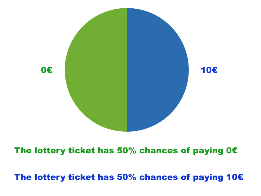
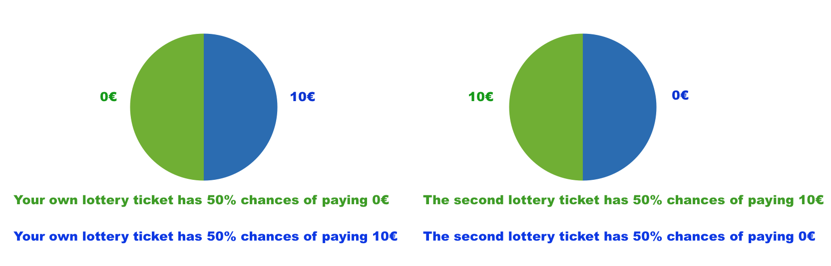
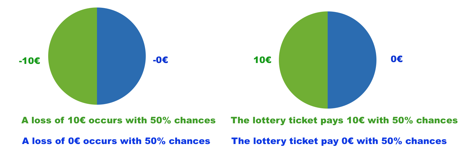
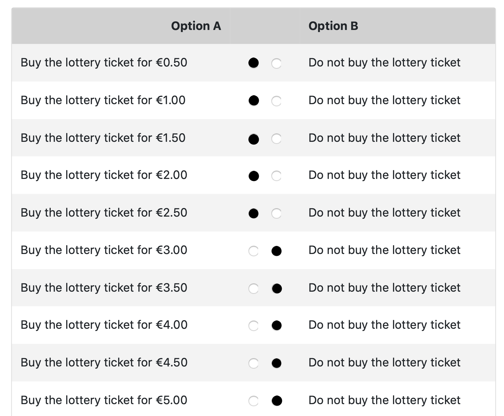

 Open access