On smooth and peaked travelling waves in a local model for shallow water waves

Abstract

We introduce a new model equation for Stokes gravity waves based on conformal transformations of Euler's equations. The local version of the model equation is relevant for the dynamics of shallow water waves. It allows us to characterize the travelling periodic waves both in the case of smooth and peaked waves and to solve the existence problem exactly, albeit not in elementary functions. Spectral stability of smooth waves with respect to co-periodic perturbations is proven analytically based on the exact count of eigenvalues in a constrained spectral problem.

1. Introduction

An irrotational motion of incompressible two-dimensional surface water waves can be fully described by means of evolution equations for two canonical variables in one spatial coordinate. This formalism was originated by Zakharov (1968) in the context of the stability of travelling periodic waves.

One approach to developing this formalism systematically is based on the Dirichlet-to-Neumann (D-N) operator (Craig & Sulem 1993). The two nonlinear evolution equations closed with the D-N operator have been studied in many works on water waves, including the recent study of modulational instability of travelling periodic waves (Berti, Maspero & Ventura 2022). See also Creedon & Deconinck (2023), Hur & Yang (2023) and Nguyen & Strauss (2023) for other recent works where three more methods have been explored in the same context.

Another approach to obtaining a closed system of two nonlinear evolution equations for water waves is based on a conformal transformation which maps the fluid domain with a variable surface profile to a fixed rectangular domain. This formalism was introduced in Babenko (1987) and Tanveer (1991) and has been explored in the context of travelling periodic waves in Dyachenko et al. (1996), Zakharov & Dyachenko (1996), Choi & Camassa (1999) and more recently in Dyachenko, Lushnikov & Korotkevich (2016), Dyachenko & Semenova (2023a,b), Korotkevich et al. (2023) and Lushnikov, Dyachenko & Silantyev (2017). Our work contributes to the analysis of the nonlinear evolution equations obtained in the latter approach.

The approach based on conformal transformations has been used to tackle many mathematical problems related to water waves such as the existence of standing waves (Wilkening 2020, 2021) and bifurcations of quasi-periodic wave solutions from the standing periodic waves (Wilkening & Zhao 2021, 2023a,b). Holomorphic coordinates were used for analysis of the well posedness of the water wave equations (Hunter, Ifrim & Tataru 2016; Harrop–Griffiths, Ifrim & Tataru 2017). The particular problem addressed in our work is the coexistence of smooth and peaked travelling periodic waves for different intervals of wave speeds as well as the linear stability of waves with smooth profiles.

1.1. A new model equation

The purpose of this paper is to introduce a new model equation which shares the same solutions as the travelling wave reduction of Euler's equations in Babenko (1987) but simplifies the time evolution and, particularly, the linear stability analysis of the travelling periodic waves. This model equation can be written in the following non-local form:

(1.1)\begin{equation} 2 c T_h^{-1} \partial_t \eta = (c^2 K_h -1) \eta - \eta K_h \eta - \tfrac{1}{2} K_h \eta^2, \end{equation}

where $\eta = \eta (u,t) \in \mathbb {R}$ is the surface elevation in the reference frame moving with the constant wave speed $c > 0$, $t \in \mathbb {R}$ is time and $u$ is the spatial coordinate defined on the periodic domain $\mathbb {T} = \mathbb {R} \backslash (2{\rm \pi} \mathbb {Z})$. The spatial coordinate $u$ arises after the conformal transformation of the fluid domain with variable surface elevation $\eta$ to a rectangle $[-{\rm \pi},{\rm \pi}] \times [-h,0]$, where $h > 0$ is the fluid depth. The linear skew–adjoint operator $T_h^{-1}$ in $L^2(\mathbb {T})$ is defined by the Fourier symbol

(1.2) \begin{equation} \widehat{(T_h^{-1})}_n = \left\{\begin{array}{@{}cl@{}} -{\rm i} \coth(hn), & n \in \mathbb{Z} \backslash \{0\}, \\ 0, & n = 0, \end{array}\right. \end{equation}

whereas the linear, self-adjoint, positive operator $K_h = T_h^{-1} \partial _u$ in $L^2(\mathbb {T})$ is defined by the Fourier symbol

(1.3) \begin{equation} \widehat{(K_h)}_n = \left\{\begin{array}{@{}cl@{}} n \coth(hn), & n \in \mathbb{Z} \backslash \{0\}, \\ 0, & n = 0. \end{array}\right. \end{equation}

Appendix A explains how the non-local evolution equation (1.1) arises in the context of the original Euler's equations.

Let us obtain the conserved quantities for the non-local model (1.1). Taking the mean value of (1.1), we get the constraint

(1.4)\begin{equation} \oint \eta (1 + K_h \eta)\,{\rm d} u = 0, \end{equation}

which represents the zero-mean constraint for the surface elevation $\eta$ in the physical spatial coordinate. Furthermore, differentiating (1.1) in $u$, multiplying by $\eta$ and integrating over the period of $\mathbb {T}$ yields

(1.5)\begin{align} c \frac{{\rm d}}{{\rm d} t} \oint \eta K_h \eta\,{\rm d} u &= \oint (c^2 \eta K_h \eta_u - \eta \eta_u - \eta \eta_u K_h \eta - \eta^2 K_h \eta_u - \eta K_h \eta \eta_u )\,{\rm d} u \nonumber\\ &= \oint \partial_u \left(\tfrac{1}{2} c^2 \eta K_h \eta - \tfrac{1}{2} \eta^2 - \eta^2 K_h \eta \right) {\rm d} u = 0, \end{align}

where we have used self-adjointness of $K_h$ in $L^2(\mathbb {T})$ for every solution with $\eta, \eta _u, \eta \eta _u$ in the domain of $K_h$. It follows from (1.4) and (1.5) that the non-local evolution equation (1.1) admits two conserved quantities

(1.6a,b)\begin{equation} \oint \eta \,{\rm d} u \quad {\rm and} \quad \oint \eta K_h \eta \,{\rm d} u. \end{equation}

In addition, the evolution equation (1.1) can be written in the Hamiltonian form

(1.7)\begin{equation} 2c T_h^{-1} \partial_t \eta = \varLambda'_c(\eta), \quad {\rm with}\ \varLambda_c(\eta) := \tfrac{1}{2} \oint [c^2 \eta K_h \eta - \eta^2 (1 + K_h \eta)]\,{\rm d} u, \end{equation}

where $\varLambda _c(\eta )$ is the action related to the conserved energy of the fluid. Critical points of $\varLambda _c$ in the corresponding energy space satisfy the Euler–Lagrange equation

(1.8)\begin{equation} (c^2 K_h - 1) \eta = \tfrac{1}{2} K_h \eta^2 + \eta K_h \eta, \end{equation}

which is known as Babenko's equation because it coincides with the travelling wave reduction of Euler's equations after the conformal transformation (Babenko 1987). In the context of the evolution equation (1.1) with $u$ defined in the reference frame moving with the wave speed $c$, solutions of (1.8) correspond to the time-independent solutions of (1.1).

1.2. Local model and main results

In the deep water limit ($h \to \infty$), we have from (1.2) and (1.3) that

(1.9a,b)\begin{equation} \lim_{h \to \infty} T_h^{-1} =-\mathcal{H} \quad {\rm and} \quad \lim_{h \to \infty} K_h =-\mathcal{H} \partial_u, \end{equation}

where $\mathcal {H}$ is the periodic Hilbert transform defined by the Fourier symbol

(1.10)\begin{equation} \hat{\mathcal{H}}_n = {\rm i}\, {\rm sgn}(n),\quad n \in \mathbb{Z}. \end{equation}

This work explores the shallow water limit ($h \to 0$), when we replace $T_h^{-1}$ and $K_h$ by $-\partial _u$ and $-\partial _u^2$, respectively. In other words, we study herein the local evolution equation

(1.11)\begin{equation} 2 c \partial_u \partial_t \eta = (c^2 - 2 \eta) \partial^2_u \eta - (\partial_u \eta)^2 + \eta. \end{equation}

Appendix B describes how the local model (1.11) arises from $T_h^{-1}$ and $K_h$ as $h \to 0$ and compares it with other phenomenological models for fluid dynamics.

It is important to emphasize that (1.11) is not the asymptotic reduction of (1.1) as $h \to 0$ but rather a toy model to understand the existence and linear stability of travelling periodic waves in the shallow water limit.

The local equation (1.11) without the last term was derived in Hunter & Saxton (1991) in a different (geometric) context and has been referred to as the Hunter–Saxton equation (Hunter & Zheng 1994). The same equation (1.11) with the last term was also discussed in Alber et al. (1995, 1999) in connection to the high-frequency limit of the Camassa–Holm equation, one of the toy models for the physics of fluids with smooth and peaked waves. Integrability of (1.11) was established in Hone, Novikov & Wang (2018) together with other peaked wave equations such as the reduced Ostrovsky and short-pulse equations. Some travelling wave solutions of this and similar equations were studied with Hirota's bilinear method in Matsuno (2020).

Next, we discuss the time evolution and the conserved quantities for the local model (1.11). Taking the mean value of (1.11) for smooth $2{\rm \pi}$-periodic solutions and integrating by parts yields the constraint

(1.12)\begin{equation} \oint [\eta + (\partial_u \eta)^2]\,{\rm d} u = 0, \end{equation}

which corresponds to (1.4) also after integration by parts. Let $\varPi _0 : L^2(\mathbb {T}) \rightarrow L^2(\mathbb {T}) |_{\{1\}^T}$ be a projection operator to the periodic functions with zero mean. The evolution equation (1.11) can be written in the form

(1.13)\begin{equation} 2 c \partial_t \eta = (c^2 - 2 \eta) \partial_u \eta + \varPi_0 \partial_u^{-1} \varPi_0 [(\partial_u \eta)^2 + \eta], \end{equation}

where $\varPi _0 \partial _u^{-1} \varPi _0$ is uniquely defined on the zero-mean functions in $L^2(\mathbb {T})$ with the zero-mean constraint. The evolution equation (1.13) is a non-local version of the inviscid Burgers equation. The initial-value problem for the inviscid Burgers equation is locally well posed in $H^1_{per}(\mathbb {T}) \cap W^{1,\infty }(\mathbb {T})$. Since the mapping

(1.14)\begin{equation} \varPi_0 \partial_u^{-1} \varPi_0 [(\partial_u \eta)^2 + \eta]: H^1_{per}(\mathbb{T}) \cap W^{1,\infty}(\mathbb{T}) \to H^1_{per}(\mathbb{T}) \cap W^{1,\infty}(\mathbb{T}) \end{equation}

is bounded on every bounded subset, there exists a unique local solution of the evolution equation (1.13) for every initial data in $H^1_{per}(\mathbb {T}) \cap W^{1,\infty }(\mathbb {T})$.

To get the conserved quantities, we multiply (1.11) by $\partial _u \eta$ and integrate over the period for smooth $2{\rm \pi}$-periodic solutions $\eta$. This implies the conservation of

(1.15)\begin{equation} Q(\eta) := \oint (\partial_u \eta)^2 \,{\rm d} u, \end{equation}

and, in view of the constraint (1.12), the conservation of

(1.16)\begin{equation} M(\eta) := \oint \eta \,{\rm d} u. \end{equation}

The conserved quantities (1.15) and (1.16) correspond to (1.6a,b). Furthermore, similar to (1.7), we can write (1.13) in the Hamiltonian form

(1.17)\begin{equation} 2c \partial_t \eta =- \varPi_0 \partial_u^{-1} \varPi_0 \left[\tfrac{1}{2} c^2 Q'(\eta) - \tfrac{1}{2} H'(\eta) \right], \end{equation}

where $H$ is the third conserved quantity given by

(1.18)\begin{equation} H(\eta) := \oint [\eta^2 + 2 \eta (\partial_u \eta)^2]\,{\rm d} u. \end{equation}

The existence of travelling periodic waves in the local model (1.11) is defined by the second-order equation

(1.19)\begin{equation} (c^2 - 2 \eta) \eta'' - (\eta')^2 + \eta = 0,\quad u \in \mathbb{T}, \end{equation}

where $\eta = \eta (u)$ is the $2{\rm \pi}$-periodic wave profile satisfying the constraint (1.12). The linear stability of the travelling wave with the profile $\eta$ is defined by the linearized equation

(1.20a,b)\begin{equation} 2 c \partial_t \hat{\eta} =-\varPi_0 \partial_u^{-1} \varPi_0 \mathcal{L} \hat{\eta},\quad \mathcal{L} :=-\partial_u (c^2 - 2 \eta) \partial_u - 1 + 2 \eta'', \end{equation}

where $\hat {\eta } = \hat {\eta }(u,t)$ is the perturbation to the travelling wave with the profile $\eta = \eta (u)$ satisfying the orthogonality condition $\langle 1 - 2 \eta '', \hat {\eta } \rangle = 0$ with the standard inner product in $L^2(\mathbb {T})$. The orthogonality condition $\langle 1 - 2 \eta '', \hat {\eta } \rangle = 0$ follows by expanding the nonlinear constraint (1.12) near $\eta$.

The following two theorems describe the main results of this work. Our results are formulated for the single-lobe periodic solutions with an even profile $\eta$ which possesses a single maximum on $\mathbb {T}$ placed at $u = 0$. Such single-lobe periodic solutions are often referred to as Stokes waves.

Theorem 1.1 There exist $c_* := {\rm \pi}/(2\sqrt{2})$ and $c_{\infty } \in (c_*,\infty )$ such that the stationary equation (1.19) admits a unique single-lobe solution with the profile $\eta \in C^{\infty }_{per}(\mathbb {T})$ for every $c \in (1,c_*)$ such that

(1.21)\begin{equation} \| \eta \|_{L^{\infty}} \to 0 \quad {\rm as}\ c \to 1 , \end{equation}

and a single-lobe solution with the profile $\eta \in C^0_{per}(\mathbb {T})$ for every $c \in (c_*,c_{\infty })$ satisfying

(1.22)\begin{equation} \eta(u) = \frac{c^2}{2} - A(c) |u|^{2/3} + O(|u|^{4/3}) \quad {\rm as}\ u \to 0, \end{equation}

for some constant $A(c) > 0$. At $c = c_*$, there exists a unique single-lobe solution with the profile $\eta \in C^0_{per}(\mathbb {T}) \cap W^{1,\infty }(\mathbb {T})$ given explicitly as

(1.23)\begin{equation} \eta(u) = \tfrac{1}{16} ( {\rm \pi}^2 - 4 {\rm \pi}|u| + 2 u^2),\quad u \in [-{\rm \pi},{\rm \pi}], \end{equation}

and extended as a $2{\rm \pi}$-periodic function on $\mathbb {T}$.

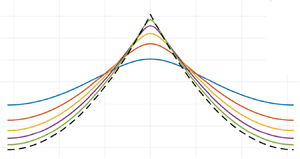
Remark 1.1 Figure 1 shows profiles of the periodic waves of Theorem 1.1. The profiles were obtained numerically by using solutions of the second-order equation (1.19).

Figure 1. Profiles in the family of smooth periodic waves (a) and singular periodic waves (b) vs $u$ for different values of wave speeds $c \in (1,c_*)$ and $c \in (c_*,c_{\infty })$, respectively. The dashed line shows the profile of the peaked periodic wave (1.23).

Remark 1.2 There exists another single-lobe solution with the singular behaviour (1.22) for every $c \in (0,c_{\infty })$ which is not included in the statement of Theorem 1.1 as it does not bifurcate from the zero solution as $c \to 1$ compared with (1.21). See figure 2 for the bifurcation diagram of all single-lobe solutions of (1.19).

Figure 2. Dependence of $E := \| \eta \|_{L^{\infty }}$ vs wave speed $c$ for periodic solutions of (1.19). The smooth solutions of Theorem 1.1 exist between the black dots. The singular solutions of Theorem 1.1 exist between the rightmost black and red dots. The singular solutions which are not included in the statement of Theorem 1.1 exist between the red dots.

Remark 1.3 The special solution (1.23) has a peaked profile with a finite jump of the first derivative. It is usually referred to as the peaked periodic wave. Such peaked periodic waves are commonly known in other fluid models such as the reduced Ostrovsky equation (Geyer & Pelinovsky 2019, 2020; Bruell & Dhara 2021), the Camassa–Holm equation (Madiyeva & Pelinovsky 2021) and the Degasperis–Procesi equation (Geyer & Pelinovsky 2024).

Remark 1.4 The singular behaviour (1.22) corresponds to the singularity of the limiting Stokes wave with a $120^{\rm o}$ angle in the physical coordinate after the conformal transformation. The behaviour was rigorously proven for the original Euler's equation in Amick, Fraenkel & Toland (1982), Plotnikov (2002) and Toland (1978), with many asymptotic results known in the literature (see Lushnikov (2016) and references therein). Note that

(1.24)\begin{equation} \max_{u \in \mathbb{T}} \eta(u) = \eta(0) = \frac{c^2}{2} \end{equation}

holds for every limiting Stokes wave for which the horizontal velocity at the wave height coincides with the wave speed $c$, see the second equation in system (A3) of Appendix A.

Theorem 1.2 Consider the unique single-lobe solution with the profile $\eta \in C^{\infty }_{per}(\mathbb {T})$ in Theorem 1.1 for $c \in (1,c_*)$. For every initial data $\hat {\eta }_0 \in H^1_{per}(\mathbb {T})$ satisfying

(1.25a,b)\begin{equation} \langle 1, \hat{\eta}_0 \rangle = 0 \quad {\rm and}\quad \langle \eta'', \hat{\eta}_0 \rangle = 0, \end{equation}

there exists a unique solution $\hat {\eta } \in C^0(\mathbb {R},H^1_{per}(\mathbb {T}))$ of the linearized equation ( 1.20 a,b) with $\hat {\eta } |_{t = 0} = \hat {\eta }_0$ and a unique $a \in C^1(\mathbb {R},\mathbb {R})$ such that

(1.26a,b)\begin{equation} \| \hat{\eta}({\cdot},t) - a(t) \eta' \|_{H^1_{per}} \leq C \| \hat{\eta}_0 \|_{H^1_{per}}, \quad |a'(t)| \leq C \| \hat{\eta}_0 \|_{H^1_{per}}, \quad t \in \mathbb{R}, \end{equation}

where $C > 0$ is independent of $\hat {\eta }_0$.

Remark 1.5 Constraints (1.25a,b) are preserved in the time evolution of the linearized equation (1.20a,b) because they are linearizations of the conserved quantities (1.15) and (1.16). In view of the constraint $\langle 1 - 2 \eta '', \hat {\eta } \rangle = 0$ imposed on solutions of the linearized equation (1.20a,b), only one constraint in (1.25a,b) is linearly independent. Imposing $\langle \eta '', \hat {\eta }_0 \rangle = 0$ is equivalent to the requirement that the perturbation $\hat {\eta }$ does not change the conserved quantity $Q$ in (1.15) up to the linear approximation. The bound (1.26a,b) expresses the concept of linear orbital stability of the orbit $\{ \eta ({\cdot } + \mathfrak {u}) \}_{\mathfrak {u} \in \mathbb {T}}$ of the travelling periodic wave with the profile $\eta$.

Remark 1.6 The linear orbital stability of Theorem 1.2 implies spectral stability of the travelling periodic wave in the sense that the spectrum of the associated linearized operator $\partial _u^{-1} \mathcal {L}$ in $L^2(\mathbb {T})$ belongs to $i \mathbb {R}$. It is also worthwhile to point out that an eigenfunction $\hat {\eta }_0$ of the spectral stability problem

(1.27)\begin{equation} \partial_u^{-1} \mathcal{L} \hat{\eta}_0 = \lambda_0 \hat{\eta}_0,\quad \eta_0 \in H^1_{per}(\mathbb{T}) \end{equation}

for every non-zero eigenvalue $\lambda _0 \in \mathbb {C} \backslash \{0\}$ must satisfy the two constraints in (1.25a,b). The spectral stability problem in the form (1.27) was also considered in Stanislavova & Stefanov (2016).

Remark 1.7 The proof of Theorem 1.2 relies on the construction of the coercive quadratic form $\langle \mathcal {L}\hat {\eta }, \hat {\eta } \rangle$ for $\hat {\eta } \in H^1_{per}(\mathbb {T})$ under the three constraints

(1.28)\begin{equation} \langle 1, \hat{\eta} \rangle = \langle \eta', \hat{\eta} \rangle = \langle \eta'', \hat{\eta} \rangle = 0. \end{equation}

The quadratic form is invariant in the time evolution of the linearized equation (1.20a,b). This yields the energetic stability of the travelling periodic wave, ensuring that the periodic wave with the profile $\eta$ is a local minimizer of the energy $H$ subject to fixed $Q$ and $M$ in $H^1_{per}(\mathbb {T})$. If local well posedness of the nonlinear evolution equation (1.13) can be shown in $H^1_{per}(\mathbb {T})$, then the energetic stability implies the nonlinear orbital stability of the travelling periodic wave. However, the local well posedness of (1.13) holds only in $H^1_{per}(\mathbb {T}) \cap W^{1,\infty }(\mathbb {T})$ and the control of $\| \partial _u \hat {\eta } \|_{L^{\infty }}$ for the perturbation $\hat {\eta }$ does not follow from the conserved quantities (1.15), (1.16) and (1.18).

1.3. Discussion

The local model (1.11) shows a pattern of the existence and stability of travelling periodic waves parameterized by the wave speed $c$. There is a continuum of wave speeds for the smooth waves with profile $\eta \in C^{\infty }(\mathbb {T})$ bifurcating from the linear limit in (1.21) and a continuum of wave speeds for the cusped waves with the profile $\eta \in C^0(\mathbb {T})$ satisfying (1.22). The two continuous families are connected together at a particular value of the wave speed $c = c_*$ for which the wave is peaked with the profile $\eta \in C^0(\mathbb {T}) \cap W^{1,\infty }(\mathbb {T})$. The same phenomenon is observed in the Camassa–Holm equation (Lenells 2005b; Geyer et al. 2022) and the Degasperis–Procesi equation (Lenells 2005a; Geyer & Pelinovsky 2024).

It is rather remarkable that exactly the same $|u|^{2/3}$ singularity in the limiting wave profile with

(1.29)\begin{equation} \max_{u \in \mathbb{T}} \eta(u) = \eta(0) = \frac{c^2}{2} \end{equation}

is recovered by the local model (1.11) as predicted by the full model for any depth $h$ (Plotnikov 2002). After the conformal transformation, this singularity yields the limiting Stokes wave with the $120^o$ angle in the physical coordinates. More precise details of such singular profiles are beyond the current capacities of the asymptotic (Lushnikov 2016) or numerical (Dyachenko et al. 2016; Lushnikov et al. 2017) methods. The local model (1.11) gives precise conclusions that the $|u|^{2/3}$ singularity is obtained in a range of wave speeds $c$ and that the borderline wave profile $\eta \in H^1_{per}(\mathbb {T}) \cap W^{1,\infty }(\mathbb {T})$ has a peaked profile at $c = c_*$ before getting the $|u|^{2/3}$ singularity for $c > c_*$. This might be an artefact of the local model (1.11) since the non-local models typically predict only the $|u|^{2/3}$ singularity in the fluid models, see Locke & Pelinovsky (2025).

Stability of the travelling periodic waves with singular profiles is a complicated problem, which is out of reach in the current analytical and numerical methods in the non-local models (Dyachenko & Semenova 2023a; Korotkevich et al. 2023). The local model (1.11) is a promising candidate for showing linear instability of the peaked wave (based on a similar analysis in Geyer & Pelinovsky 2019, 2020; Madiyeva & Pelinovsky 2021) and for attacking linear instability of the cusped wave with the $|u|^{2/3}$ singularity.

The remainder of this paper is organized as follows. Section 2 contains the proof of Theorem 1.1 on the existence of smooth and peaked periodic waves. Section 3 gives the proof of Theorem 1.2 on linear stability of the smooth periodic waves. Appendix A reviews the Euler equations after the conformal transformation and discusses how the non-local model (1.1) arises. Appendix B describes the local model (1.11) in the context of other phenomenological models for dynamics of fluid surfaces.

2. Existence of smooth and peaked travelling periodic waves

We consider the single-lobe periodic solutions of the second-order equation (1.19). Recall that a single-lobe periodic solution has the even profile $\eta$ with a single maximum on $\mathbb {T}$ placed at $u = 0$. Theorem 1.1 is proven by using the period function for the planar Hamiltonian systems used in a similar context in Geyer et al. (2022), Geyer & Pelinovsky (2017, 2024) and Long & Liu (2023).

We start with the first-order invariant of the second-order equation (1.19) given by the following lemma.

Lemma 2.1 For every solution $\eta \in C^2(a,b)$ of the second-order equation (1.19) with $-\infty \leq a < b \leq \infty$, the following function:

(2.1)\begin{equation} E(\eta,\eta') := \tfrac{1}{2} (c^2 - 2 \eta) (\eta')^2 + \tfrac{1}{2} \eta^2 \end{equation}

is constant for $u \in (a,b)$.

Proof. It is based on the elementary computation

(2.2)\begin{align} \frac{{\rm d}}{{\rm d} u} E(\eta,\eta') &= (c^2 - 2 \eta) \eta' \eta'' - (\eta')^3 + \eta \eta' \nonumber\\ &= \eta' [(c^2 - 2 \eta) \eta'' - (\eta')^2 + \eta] \nonumber\\ &= 0, \end{align}

since $\eta \in C^2(a,b)$ satisfies (1.19).

The next lemma explores the phase portrait for the second-order equation (1.19) on the phase plane $(\eta,\eta ')$ obtained from the level curves of $E(\eta,\eta ')$ in (2.1). We obtain the existence of smooth and singular solutions in terms of the level $\mathcal {E}$ of $E(\eta,\eta ')$.

Lemma 2.2 For every $c > 0$, there exists $\mathcal {E}_c := {c^4}/{8}$ such that every periodic solution to (1.19) with profile $\eta \in C^{\infty }(\mathbb {R})$ belongs to $E(\eta,\eta ') = \mathcal {E}$ with $\mathcal {E}\in (0,\mathcal {E}_c)$. For $E(\eta,\eta ') = \mathcal {E}_c$, the only solution to (1.19) is the parabola

(2.3)\begin{equation} \eta(u) =-\frac{c^2}{2} + \frac{(u-u_0)^2}{8}, \end{equation}

with arbitrary $u_0 \in \mathbb {R}$. For $E(\eta,\eta ') = \mathcal {E}$ with $\mathcal {E}\in (\mathcal {E}_c,\infty )$, there exist no bounded solutions to (1.19) with profile $\eta \in C^{\infty }(\mathbb {R})$.

Proof. The only equilibrium point of (1.19) is the centre $(\eta,\eta ') = (0,0)$, which corresponds to the minimum of $E(\eta,\eta ')$ if $c > 0$. Every periodic solution to (1.19) belongs to the period annulus, which is the largest punctured neighbourhood of the centre $(0,0)$ consisting entirely of periodic orbits.

The phase portrait from the level curves of $E(\eta,\eta ') = \mathcal {E}$ is shown on figure 3. Each level curve defines the profile $\eta$ from integration of

(2.4)\begin{equation} \left(\frac{{\rm d} \eta}{{\rm d} u} \right)^2 = \frac{2 \mathcal{E} - \eta^2}{c^2 - 2 \eta}. \end{equation}

The vertical line corresponds to $\eta = {c^2}/{2}$ and divides the phase plane into two half-planes. For $\eta > {c^2}/{2}$, the level curves of $E(\eta,\eta ') = \mathcal {E}$ contain no bounded solutions. For $\eta < {c^2}/{2}$, bounded level curves exist for $\mathcal {E}\in (0,\mathcal {E}_c)$ with $\mathcal {E}_c := {c^4}/{8}$ and contain periodic solutions with profile $\eta \in C^{\infty }(\mathbb {R})$. For $\mathcal {E} = \mathcal {E}_c$, all solutions are given by integrating

(2.5)\begin{equation} \left(\frac{{\rm d} \eta}{{\rm d} u} \right)^2 = \frac{2 \mathcal{E}_c - \eta^2}{c^2 - 2 \eta} = \tfrac{1}{4} (c^2 + 2 \eta). \end{equation}

Differentiating in $u$ gives $\eta ''(u) = \frac {1}{4}$. Integrating twice and using (2.5) yields (2.3) with profile $\eta \in C^{\infty }(\mathbb {R})$. Finally, for $\mathcal {E} > \mathcal {E}_c$, the level curve reaches $\eta = {c^2}/{2}$ with the singularity of $\eta '$, which rules out the existence of bounded solutions with profile $\eta \in C^{\infty }(\mathbb {R})$.

Figure 3. Phase portrait from the level curves of $E(\eta,\eta ') = \mathcal {E}$ for $c = 1$.

The next lemma clarifies how the solutions for $\eta < {c^2}/{2}$ reach the singularity line $\eta = {c^2}/{2}$.

Lemma 2.3 Let $\eta \in C^0(u_-,u_+)$ be a solution for the level curve $E(\eta,\eta ') = \mathcal {E}$ for $\mathcal {E} \in (\mathcal {E}_c,\infty )$ such that $\eta (u) \to \pm {c^2}/{2}$ as $u \to u_{\pm }$. Then, $-\infty < u_- < u_+ < \infty$ and the solution satisfies

(2.6)\begin{equation} \eta(u) = \frac{c^2}{2} - \frac{3^{2/3}}{2^{2/3}} (\mathcal{E} - \mathcal{E}_c)^{1/3} |u-u_{{\pm}}|^{2/3} + O(|u-u_{{\pm}}|^{4/3})\quad {\rm as}\ u \to u_{{\pm}}. \end{equation}

Proof. We consider the level curve $E(\eta,\eta ') = \mathcal {E}$ with $\mathcal {E} \in (\mathcal {E}_c,\infty )$ for $\eta < {c^2}/{2}$. Then, we have

(2.7)\begin{align} \left(\frac{{\rm d} \eta}{{\rm d} u} \right)^2 &= \frac{2 \mathcal{E} - \eta^2}{c^2 - 2 \eta} \nonumber\\ &= \frac{2(\mathcal{E} - \mathcal{E}_c)}{c^2 - 2 \eta} + \frac{1}{2} c^2 + \frac{1}{4} (2 \eta - c^2) \nonumber\\ &= \frac{2(\mathcal{E} - \mathcal{E}_c)}{c^2 - 2 \eta} + O(1) \quad {\rm as}\ \eta \to \frac{c^2}{2}. \end{align}

This yields

(2.8)\begin{equation} \sqrt{c^2 - 2 \eta} [1 + O(|c^2-2\eta|)] \frac{{\rm d} \eta}{{\rm d} u} ={\pm} \sqrt{2 (\mathcal{E} - \mathcal{E}_c)} \quad {\rm as}\ u \to u_{{\pm}} \mp 0. \end{equation}

Integrating in $u$ yields

(2.9)\begin{equation} \sqrt{(c^2 - 2 \eta)^3} [1 + O(|c^2-2\eta|)]={\mp} 3 \sqrt{2 (\mathcal{E} - \mathcal{E}_c)} (u - u_{{\pm}}) \quad {\rm as}\ u \to u_{{\pm}} \mp 0, \end{equation}

which results in the expansion (2.6). It remains to prove that $[u_-,u_+]$ is compact. This follows from the bounds

(2.10)\begin{align} u_+- u_- &= 2 \int_{-\sqrt{2 \mathcal{E}}}^{c^2/2} \frac{\sqrt{c^2 - 2 \eta}}{\sqrt{2 \mathcal{E} - \eta^2}} {\rm d} \eta \nonumber\\ &\leq 2 \sqrt{c^2 +2 \sqrt{2 \mathcal{E}}} \int_{-\sqrt{2 \mathcal{E}}}^{c^2/2} \frac{{\rm d}\eta}{\sqrt{2 \mathcal{E} - \eta^2}} < \infty, \end{align}

since the integral in the upper bound is finite.

In order to analyse bounded periodic solutions in Lemma 2.2, we introduce the following period function associated with (2.1) and (2.4):

(2.11)\begin{equation} T(\mathcal{E},c) := 2 \int_{-\sqrt{2 \mathcal{E}}}^{\sqrt{2 \mathcal{E}}} \frac{\sqrt{c^2 - 2 \eta}}{\sqrt{2 \mathcal{E} - \eta^2}} {\rm d} \eta,\quad \mathcal{E}\in (0,\mathcal{E}_c). \end{equation}

For the singular solutions in Lemma 2.3, we augment the period function for $\mathcal {E} \geq \mathcal {E}_c$ as

(2.12)\begin{equation} T(\mathcal{E},c) := 2 \int_{-\sqrt{2 \mathcal{E}}}^{c^2/2} \frac{\sqrt{c^2 - 2 \eta}}{\sqrt{2 \mathcal{E} - \eta^2}} {\rm d} \eta,\quad \mathcal{E}\in [\mathcal{E}_c,\infty). \end{equation}

The next result describes properties of the period function $(0,\infty ) \ni \mathcal {E} \mapsto T(\mathcal {E},c)$ for every fixed $c > 0$.

Lemma 2.4 For every $c > 0$, there exist $\mathcal {E}_*, \mathcal {E}_{**} \in (\mathcal {E}_c,\infty )$ that depend on $c$ such that

(2.13)\begin{equation} \frac{\partial}{\partial \mathcal{E}} T(\mathcal{E},c) < 0,\quad \mathcal{E} \in (0,\mathcal{E}_*), \end{equation}

and

(2.14)\begin{equation} \frac{\partial}{\partial \mathcal{E}} T(\mathcal{E},c) > 0,\quad \mathcal{E} \in (\mathcal{E}_{**},\infty), \end{equation}

with

(2.15)\begin{equation} \left.\begin{gathered} T(\mathcal{E},c) \to 2 {\rm \pi}c \quad {\rm as}\ \mathcal{E} \to 0, \\ T(\mathcal{E},c) \to 4 \sqrt{2} c \quad {\rm as}\ \mathcal{E} \to \mathcal{E}_c, \end{gathered}\right\} \end{equation}

and $T(\mathcal {E},c) \to \infty$ as $\mathcal {E}\to \infty$. In addition, we have

(2.16)\begin{equation} \frac{\partial}{\partial c} T(\mathcal{E},c) > 0,\quad \mathcal{E} \in (0,\infty),\enspace c \in (0,\infty). \end{equation}

Proof. For the smooth periodic solutions, we use the change of variables $\eta = \sqrt {2 \mathcal {E}} x$ in (2.11) and obtain

(2.17)\begin{equation} T(\mathcal{E},c) = 2 \int_{-1}^{1} \frac{\sqrt{c^2 - 2 \sqrt{2 \mathcal{E}} x}}{\sqrt{1 - x^2}}{{\rm d}\kern0.06em x},\quad \mathcal{E}\in (0,\mathcal{E}_c). \end{equation}

Since the weak singularity is independent of $\mathcal {E}$, we can differentiate under the integration sign and obtain

(2.18)\begin{equation} \frac{\partial}{\partial \mathcal{E}} T(\mathcal{E},c) =-\frac{2}{\sqrt{2 \mathcal{E}}} \int_{-1}^{1} \frac{x\,{{\rm d}\kern0.06em x}}{\sqrt{1 - x^2} \sqrt{c^2 - 2 \sqrt{2 \mathcal{E}} x}},\quad \mathcal{E}\in (0,\mathcal{E}_c). \end{equation}

The result is strictly negative since

(2.19)\begin{equation} \frac{|x|}{\sqrt{1 - x^2} \sqrt{c^2 + 2 \sqrt{2 \mathcal{E}} |x|}} < \frac{x}{\sqrt{1 - x^2} \sqrt{c^2 - 2 \sqrt{2 \mathcal{E}} x}}, \quad x \in (0,1). \end{equation}

This proves (2.13) for $\mathcal {E}\in (0,\mathcal {E}_c)$. We also obtain from the same representation

(2.20)\begin{equation} T(\mathcal{E},c) \to 2c \int_{-1}^1 \frac{{\rm d}\kern0.06em x}{\sqrt{1-x^2}} = 2 {\rm \pi}c \quad {\rm as}\ \mathcal{E} \to 0 , \end{equation}

and

(2.21)\begin{equation} T(\mathcal{E},c) \to 2c \int_{-1}^1 \frac{\sqrt{1-x}}{\sqrt{1-x^2}} {{\rm d}\kern0.06em x} = 4 \sqrt{2} c \quad {\rm as}\ \mathcal{E} \to \mathcal{E}_c. \end{equation}

Monotonicity (2.16) follows from the positive derivative of (2.11) in $c$.

For the singular solutions, we break (2.12) into the sum of two terms and use the same change of variables only in the first term

(2.22)\begin{align} T(\mathcal{E},c) = 2 \int_{-1}^{-c^2/2\sqrt{2 \mathcal{E}}} \frac{\sqrt{c^2 - 2 \sqrt{2 \mathcal{E}} x}}{\sqrt{1 - x^2}} {{\rm d}\kern0.06em x} + 2 \int_{-c^2/2}^{c^2/2} \frac{\sqrt{c^2 - 2 \eta}}{\sqrt{2 \mathcal{E} - \eta^2}} {\rm d} \eta,\quad \mathcal{E}\in [\mathcal{E}_c,\infty). \end{align}

Since $8 \mathcal {E} > c^4$, both terms are differentiable under the integration sign and we obtain

(2.23)\begin{align} \frac{\partial}{\partial \mathcal{E}} T(\mathcal{E},c) =-\frac{2}{\sqrt{2 \mathcal{E}}} \int_{-1}^{-c^2/2\sqrt{2 \mathcal{E}}} \frac{x \,{{\rm d}\kern0.06em x}}{\sqrt{1 - x^2} \sqrt{c^2 - 2 \sqrt{2 \mathcal{E}} x}} - 2 \int_{-c^2/2}^{c^2/2} \frac{\sqrt{c^2 - 2 \eta}}{\sqrt{(2 \mathcal{E} - \eta^2)^3}} {\rm d} \eta, \end{align}

where the first term is positive and the second term is negative. The first term is zero as $\mathcal {E} \to \mathcal {E}_c$, monotonically increasing for $\mathcal {E} \gtrsim \mathcal {E}_c$ and monotonically decreasing as $\mathcal {E} \to \infty$. The second term is strictly negative as $\mathcal {E} \to \mathcal {E}_c$ and is monotonically increasing towards $0$ for $\mathcal {E} > \mathcal {E}_c$. Since

(2.24)\begin{equation} \int_{-1}^{-c^2/2\sqrt{2 \mathcal{E}}} \frac{\sqrt{c^2 - 2 \sqrt{2 \mathcal{E}} x}}{\sqrt{1 - x^2}} {{\rm d}\kern0.06em x} \sim (8 \mathcal{E})^{1/4} \int_{-1}^0 \frac{\sqrt{|x|}{{\rm d}\kern0.06em x}}{\sqrt{1-x^2}} \quad {\rm as}\ \mathcal{E}\to \infty , \end{equation}

and

(2.25)\begin{equation} \int_{-c^2/2}^{c^2/2} \frac{\sqrt{c^2 - 2 \eta}}{\sqrt{2 \mathcal{E} - \eta^2}} {\rm d} \eta \sim (2 \mathcal{E})^{-1/2} \int_{-c^2/2}^{c^2/2} \sqrt{c^2 - 2 \eta} {\rm d} \eta \quad {\rm as}\ \mathcal{E}\to \infty , \end{equation}

the first term in the decomposition (2.23) is larger than the second term at infinity and we have $T(\mathcal {E},c) = {O}(\mathcal {E}^{1/4})$ as $\mathcal {E} \to \infty$ so that

(2.26)\begin{equation} T(\mathcal{E},c) \to \infty \quad {\rm as}\ \mathcal{E}\to \infty. \end{equation}

At the same time, the first term in the decomposition (2.23) is zero at $\mathcal {E} = \mathcal {E}_c$, hence there exist $\mathcal {E}_*,\mathcal {E}_{**} \in (\mathcal {E}_c,\infty )$ such that (2.13) and (2.14) hold. Monotonicity (2.16) follows from the positive derivative of (2.12) in $c$.

We are now ready to prove Theorem 1.1.

Proof of Theorem 1.1 We consider the family of solutions of Lemmas 2.2 and 2.3 for $\mathcal {E}\in (0,\infty )$ and $\eta < {c^2}/{2}$. For every $c > 0$, we select the intersection of the period function $T(\mathcal {E},c)$ of Lemma 2.4 with the $2{\rm \pi}$ period on $\mathbb {T}$. It follows from (2.16) that the period function is monotonically increasing in $c$ for every $\mathcal {E} \in (0,\infty )$.

For the smooth periodic solutions with the period function (2.11), there exists only one root $\mathcal {E} \in (0,\mathcal {E}_c)$ of $T(\mathcal {E},c) = 2{\rm \pi}$ for every $c \in (1,c_*)$ with $c_* = {\rm \pi}/(2\sqrt{2})$ due to monotonicity (2.13) and the limiting values $T(0,c) = 2 {\rm \pi}c$ and $T(\mathcal {E}_c,c) = 4 \sqrt {2} c$. This gives the first assertion of the theorem with the limit (1.21) since the smooth periodic solution shrinks to the centre point $(0,0)$ on the $(\eta,\eta ')$ plane as $\mathcal {E}\to 0$. At $c = c_*$, we have $\mathcal {E} = \mathcal {E}_{c_*}$ for the root of $T(\mathcal {E},c) = 2{\rm \pi}$. The unique single-lobe solution (1.23) follows from the unique solution (2.3) at $\mathcal {E} = \mathcal {E}_c$ from Lemma 2.2 by the translation $u_0 = {\rm \pi}$ for $u \in [0,{\rm \pi} ]$ and an even reflection on $[-{\rm \pi},0]$.

For the singular solutions with the period function (2.12), we have a root $\mathcal {E} \in (\mathcal {E}_c,\infty )$ of $T(\mathcal {E},c) = 2{\rm \pi}$ for every $c \in (c_*,c_{\infty })$ due to monotonicity (2.13). The value $c_{\infty }$ is obtained from the intersection of $T(\mathcal {E}_*,c)$ with $2 {\rm \pi}$. The asymptotic expansion (1.22) of the singular single-lobe solutions follows from the expansion (2.6) with the translation $u_- = 0$ of the solution in Lemma 2.3 for $u \in [0,{\rm \pi} ]$ with $\eta ({\rm \pi} ) = -\sqrt {2 \mathcal {E}}$ and $\eta '({\rm \pi} ) = 0$ and an even reflection on $[-{\rm \pi},0]$.

Figure 4 illustrates the result of Lemma 2.4 and the proof of Theorem 1.1. The period functions (2.11) and (2.12) can be computed in terms of complete elliptic integrals by using 3.141 (integrals 2 and 9) in Gradshteyn & Ryzhik (2007)

(2.27)\begin{equation} T(\mathcal{E},c) = 4 \sqrt{c^2 + 2 \sqrt{2\mathcal{E}}} E\left(\sqrt{\frac{4 \sqrt{2\mathcal{E}}}{c^2 + 2 \sqrt{2\mathcal{E}}}}\right),\quad \mathcal{E} \in (0,\mathcal{E}_c), \end{equation}

and

(2.28)\begin{align} T(\mathcal{E},c) &= 4 (2\mathcal{E})^{1/4} \left[2 E\left(\sqrt{\frac{c^2 + 2 \sqrt{2\mathcal{E}}}{4 \sqrt{2\mathcal{E}}}} \right) \right. \nonumber\\ &\quad \left.+ \left(\frac{c^2}{2 \sqrt{2 \mathcal{E}}} - 1 \right) K \left(\sqrt{\frac{c^2 + 2 \sqrt{2\mathcal{E}}}{4 \sqrt{2\mathcal{E}}}}\right)\right],\quad \mathcal{E} \in (\mathcal{E}_c,\infty), \end{align}

where $K(k)$ and $E(k)$ are complete elliptic integrals of the first and second kind, respectively. The two definitions agree at $T(\mathcal {E}_c,c) = 4 \sqrt {2} c$, where $\mathcal {E}_c = {c^4}/{8}$ shown by the black dot in figure 4. We can also see from figure 4 that the monotonicity results (2.13), (2.14) and (2.16) hold true with $\mathcal {E}_* = \mathcal {E}_{**}$. The periodic solutions of Theorem 1.1 on $\mathbb {T}$ are obtained by the intersection of the plot of the period function with the level $T(\mathcal {E},c) = 2{\rm \pi}$.

Figure 4. Period function $T$ vs $\mathcal {E}$ for $c = 1.05$ (solid blue) and $c = 1.1$ (dashed blue). Black dots show the values $T(0,c) = 2{\rm \pi} c$ and $T(\mathcal {E}_c,c) = 4 \sqrt {2}c$. The red dashed line gives the level $T(\mathcal {E},c) = 2{\rm \pi}$ for periodic solutions on $\mathbb {T}$.

3. Stability of smooth travelling periodic waves

We consider the unique single-lobe solution with the profile $\eta \in C^{\infty }_{per}(\mathbb {T})$ in Theorem 1.1 which exists in the second-order equation (1.19) for $c \in (1,c_*)$ with $c_* = {\rm \pi}/(2\sqrt{2})$. Theorem 1.2 is proven by showing that the periodic solution is a constrained minimizer of the quadratic form $\langle \mathcal {L}\hat {\eta }, \hat {\eta } \rangle$ associated with the linear operator

(3.1)\begin{equation} \mathcal{L} =-\partial_u (c^2 - 2 \eta) \partial_u - 1 + 2 \eta'', \end{equation}

in the function space $H^1_{per}(\mathbb {T}) \cap \mathcal {X}_c$, where

(3.2)\begin{equation} \mathcal{X}_c := \{\hat{\eta} \in L^2(\mathbb{T}): \langle 1, \hat{\eta} \rangle = \langle \eta'', \hat{\eta} \rangle = 0\}. \end{equation}

The minimizer is only degenerate due to the translational symmetry which results in the one-dimensional kernel ${\rm Ker}(\mathcal {L}) = {\rm span}(\eta ')$ with $\eta ' \in \mathcal {X}_c$.

We start with the count of the negative eigenvalues of $\mathcal {L} : H^2_{per}(\mathbb {T}) \subset L^2(\mathbb {T}) \to L^2(\mathbb {T})$ in the following lemma.

Lemma 3.1 Let $\eta \in C^{\infty }_{per}(\mathbb {T})$ be the profile of the single-lobe solution in Theorem 1.1 for $c \in (1,c_*)$ and $\mathcal {L} : H^2_{per}(\mathbb {T}) \subset L^2(\mathbb {T}) \to L^2(\mathbb {T})$ be the linear operator given by (3.1). Then, $\mathcal {L}$ has two simple negative eigenvalues and a simple zero eigenvalue, with the rest of its spectrum bounded away from zero.

Proof. Since $\mathcal {L} : H^2_{per}(\mathbb {T}) \subset L^2(\mathbb {T}) \to L^2(\mathbb {T})$ is a self-adjoint Sturm–Liouville operator with $\eta '' \in L^{\infty }(\mathbb {T})$ and $c^2 - 2 \eta (u) > 0$ for every $u \in \mathbb {T}$, its spectrum consists of isolated eigenvalues located on the real line.

For fixed $c \in (1,c_*)$, differentiating (1.19) in $u$ yields $\mathcal {L} \eta ' = 0$ with $\eta ' \in H^2_{per}(\mathbb {T})$. Hence, $\mathcal {L}$ admits a zero eigenvalue with the spatially odd eigenfunction $\eta '$. To consider the second linearly independent solution of $\mathcal {L} \hat {\eta } = 0$, we define the family $\{ \eta (u;\mathcal {E})\}_{\mathcal {E}\in (0,\mathcal {E}_c)}$ of spatially even, smooth periodic solutions of the second-order equation (1.19) with

(3.3a,b)\begin{equation} \eta(0;\mathcal{E}) = \sqrt{2 \mathcal{E}},\quad \partial_u \eta(0;\mathcal{E}) = 0, \end{equation}

and

(3.4a,b)\begin{equation} \eta(T(\mathcal{E},c);\mathcal{E}) = \sqrt{2 \mathcal{E}}, \quad \partial_u \eta(T(\mathcal{E},c);\mathcal{E}) = 0, \end{equation}

where $T(\mathcal {E},c)$ is the period function (2.11) satisfying (2.13). Let $\mathcal {E}(c)$ be the root of the period function $T(\mathcal {E},c) = 2{\rm \pi}$ in the proof of Theorem 1.1 such that $\eta (u) = \eta (u;\mathcal {E}(c)) \in C^{\infty }_{per}(\mathbb {T})$. Differentiating (1.19) in $\mathcal {E}$ along the family $\{ \eta (u;\mathcal {E})\}_{\mathcal {E}\in (0,\mathcal {E}_c)}$ and setting $\mathcal {E}= \mathcal {E}(c)$ yields the second linearly independent solution of $\mathcal {L} \hat {\eta } = 0$. The solution is given by the spatially even function $\partial _{\mathcal {E}} \eta ({\cdot };\mathcal {E}(c))$ which satisfies

(3.5a,b)\begin{equation} \partial_{\mathcal{E}} \eta(0;\mathcal{E}) = \frac{1}{\sqrt{2 \mathcal{E}}}, \quad \partial_u \partial_{\mathcal{E}} \eta(0;\mathcal{E}) = 0, \end{equation}

and

(3.6a,b)\begin{equation} \partial_{\mathcal{E}} \eta(T(\mathcal{E},c);\mathcal{E}) = \frac{1}{\sqrt{2 \mathcal{E}}}, \quad \partial_u \partial_{\mathcal{E}} \eta(T(\mathcal{E},c);\mathcal{E}) = \partial_{\mathcal{E}} T(\mathcal{E},c) \frac{\sqrt{2 \mathcal{E}}}{c^2 - 2 \sqrt{2 \mathcal{E}}}, \end{equation}

where we have used (1.19) at $u = T(\mathcal {E},c)$ which implies

(3.7)\begin{equation} \partial^2_u \eta(T(\mathcal{E},c);\mathcal{E}) =-\frac{\sqrt{2 \mathcal{E}}}{c^2 - 2 \sqrt{2 \mathcal{E}}}. \end{equation}

We thus have $\partial _{\mathcal {E}} \eta ({\cdot };\mathcal {E}(c)) \in H^2_{per}(\mathbb {T})$ if and only if $\partial _{\mathcal {E}} T(\mathcal {E}(c),c) = 0$, which is impossible due to monotonicity (2.13). Hence, $0$ is a simple eigenvalue of $\mathcal {L}$ bounded away from the rest of its spectrum in $L^2(\mathbb {T})$.

To prove that there exist two negative eigenvalues of $\mathcal {L}$ below the zero eigenvalue, we use Proposition 1 in Geyer et al. (2022) and construct the following two normalized solutions:

(3.8a,b)\begin{equation} \eta_1(u) := \sqrt{2\mathcal{E}} \partial_{\mathcal{E}} \eta(u;\mathcal{E}) \quad {\rm and} \quad \eta_2(u) := \frac{\eta'(u)}{\eta''(0)}, \end{equation}

where $\eta _2(u+2{\rm \pi} ) = \eta _2(u)$ and $\eta _1(u+2{\rm \pi} ) = \eta _1(u) + \theta \eta _2(u)$ with

(3.9)\begin{equation} \theta := \partial_{\mathcal{E}} T(\mathcal{E}(c),c) \frac{\sqrt{2 \mathcal{E}(c)}}{c^2 - 2 \sqrt{2 \mathcal{E}(c)}} < 0, \end{equation}

due to monotonicity (2.13). By Proposition 1 in Geyer et al. (2022), $0$ is the third eigenvalue of $\mathcal {L}$ with two simple negative eigenvalues below $0$.

Remark 3.1 One can prove the assertion of Lemma 3.1 by using small-amplitude expansions. The periodic solution with the profile $\eta \in C^{\infty }_{per}(\mathbb {T})$ is expanded near the trivial solution, see (1.21), as

(3.10a,b)\begin{equation} \eta = a \cos(u) - a^2 \sin^2(u) + O(a^3), \quad c^2 = 1 + \tfrac{1}{2} a^2 + O(a^4), \end{equation}

where $a > 0$ is a small parameter. Then, $\mathcal {L}$ along the solution family has one negative eigenvalue $-1 + {O}(a^2)$ and a small negative eigenvalue $-a^2 + {O}(a^4)$ with $0$ being the third eigenvalue. Since ${\rm Ker}(\mathcal {L}) = {\rm span}(\eta ')$ along the family of smooth periodic solutions for $c \in (1,c_*)$, the inertia index of $\mathcal {L}$ remains the same for every $c \in (1,c_*)$.

The next lemma specifies the criterion for the constrained linear operator $\mathcal {L}|_{\mathcal {X}_c}$ to be positive, where $\mathcal {L}|_{\mathcal {X}_c} = \mathcal {L} |_{\{ 1, \eta ''\}^{\perp }}$ is defined by the two constraints in (3.2).

Lemma 3.2 Let $\mathcal {L} : H^2_{per}(\mathbb {T}) \subset L^2(\mathbb {T}) \to L^2(\mathbb {T})$ be given by (3.1) as in Lemma 3.1 and $\mathcal {X}_c$ be the constrained subspace of $L^2(\mathbb {T})$ given by (3.2). Then, $\mathcal {L}|_{\mathcal {X}_c}$ has a simple zero eigenvalue and no negative eigenvalues, with the rest of its spectrum being bounded away from zero, if and only if the mapping

(3.11)\begin{equation} (1,c_*) \ni c \mapsto \mathcal{M}(c) := \oint \eta \,{\rm d} u \end{equation}

is monotonically decreasing for $c \in (1,c_*)$.

Proof. By Proposition 2 in Geyer et al. (2022), we construct the $2$-by-$2$ matrix related to the two constraints in $\mathcal {X}_c$

(3.12)\begin{equation} A := \left[\begin{matrix} \langle \mathcal{L}^{-1} 1, 1 \rangle & \langle \mathcal{L}^{-1} 1, \eta'' \rangle \\ \langle \mathcal{L}^{-1} \eta'', 1 \rangle & \langle \mathcal{L}^{-1} \eta'', \eta'' \rangle \end{matrix}\right]. \end{equation}

The inverse operator $\mathcal {L}^{-1}$ on ${\rm span}(1,\eta '')$ is well defined since

(3.13)\begin{equation} {\rm Ker}(\mathcal{L}) = {\rm span}(\eta') \perp {\rm span}(1,\eta''). \end{equation}

Differentiating (1.19) in $c$ yields

(3.14)\begin{equation} \mathcal{L} \partial_c \eta = 2 c \eta'', \end{equation}

where $\partial _c \eta$ is defined along the family of $2{\rm \pi}$-periodic solutions $\{ \eta \}_{c \in (1,c_*)}$. The family is smooth in $c$ since $T(\mathcal {E},c)$ is $C^1$ on $(0,\mathcal {E}_c) \times (0,c_*)$ and $\mathcal {E}(c)$ is $C^1$ on $(0,c_*)$ due to the implicit function theorem for $T(\mathcal {E}(c),c) = 2{\rm \pi}$ with $\partial _{\mathcal {E}} T(\mathcal {E}(c),c) < 0$. In addition, we have $\mathcal {L} 1 = 2 \eta '' - 1$ so that

(3.15)\begin{equation} \mathcal{L} (c^{-1} \partial_c \eta - 1) = 1. \end{equation}

By using (3.14) and (3.15), we compute

(3.16)\begin{equation} A = \left[\begin{matrix} c^{-1} \langle \partial_c \eta, 1 \rangle - 2{\rm \pi} & c^{-1} \langle \partial_c \eta, \eta'' \rangle \\ (2c)^{-1} \langle \partial_c \eta, 1 \rangle & (2c)^{-1} \langle \partial_c \eta, \eta'' \rangle \end{matrix}\right]. \end{equation}

Since $A$ is symmetric, we have $\langle \partial _c \eta, 1 \rangle = 2 \langle \partial _c \eta, \eta '' \rangle$. Furthermore,

(3.17)\begin{equation} \det(A) =- \frac{\rm \pi}{2 c} \langle \partial_c \eta, 1 \rangle =-\frac{\rm \pi}{2c} \mathcal{M}'(c), \end{equation}

where $\mathcal {M}(c)$ is given by (3.11). Since $c > 0$, we have the following trichotomy from Proposition 2 in Geyer et al. (2022):

1. (i) If $\mathcal {M}'(c) > 0$, then $\det (A) < 0$, hence $A$ has one negative and one positive eigenvalue so that $\mathcal {L}|_{\mathcal {X}_c}$ admits one simple negative and a simple zero eigenvalue.

2. (ii) If $\mathcal {M}'(c) = 0$, then $\det (A) = 0$ but ${\rm tr}(A) < 0$, hence $A$ has one negative and one zero eigenvalue so that $\mathcal {L}|_{\mathcal {X}_c}$ admits a double zero eigenvalue and no negative eigenvalues.

3. (iii) If $\mathcal {M}'(c) < 0$, then $\det (A) > 0$, hence $A$ has two negative eigenvalues so that $\mathcal {L}|_{\mathcal {X}_c}$ admits a simple zero eigenvalue and no negative eigenvalues.

The last case yields the assertion of the lemma.

Remark 3.2 Due to constraint (1.12), we have

(3.18)\begin{equation} M(\eta) = \oint \eta \,{\rm d} u =- \oint (\partial_u \eta)^2 \,{\rm d} u =- Q(\eta), \end{equation}

so that the criterion in Lemma 3.2 is equivalent to the mapping of

(3.19)\begin{equation} (1,c_*) \ni c \mapsto \mathcal{Q}(c) := \oint (\eta')^2 \,{\rm d} u \end{equation}

being monotonically increasing for $c \in (1,c_*)$.

Since $\mathcal {M}(c) \to 0$ as $c \to 1$ by (1.21) and $\mathcal {M}(c) < 0$ by (3.18), it is clear that $\mathcal {M}'(c) < 0$ for $c \gtrsim 1$. The next lemma asserts that $\mathcal {M}'(c) < 0$ for every $c \in (1,c_*)$.

Lemma 3.3 The mapping (3.11) is monotonically decreasing for every $c \in (1,c_*)$.

Proof. Differentiating $T(\mathcal {E}(c),c) = 2{\rm \pi}$ in $c$ yields

(3.20)\begin{equation} \partial_c T(\mathcal{E}(c),c) + \mathcal{E}'(c) \partial_{\mathcal{E}} T(\mathcal{E}(c),c) = 0, \end{equation}

where

(3.21)\begin{equation} \left.\begin{gathered} \partial_c T(\mathcal{E},c) = 2c \int_{-\sqrt{2 \mathcal{E}}}^{\sqrt{2 \mathcal{E}}} \frac{{\rm d} \eta}{\sqrt{2 \mathcal{E} - \eta^2} \sqrt{c^2 - 2 \eta}}, \\ \partial_{\mathcal{E}} T(\mathcal{E},c) =-\mathcal{E}^{-1} \int_{-\sqrt{2 \mathcal{E}}}^{\sqrt{2 \mathcal{E}}} \frac{\eta {\rm d} \eta}{\sqrt{2 \mathcal{E} - \eta^2} \sqrt{c^2 - 2 \eta}}, \end{gathered}\right\} \end{equation}

and we have used (2.18) with the substitution $\eta = \sqrt {2 \mathcal {E}}x$. By using the same substitution, we define $\mathcal {M}(c) \equiv \mathcal {M}(\mathcal {E}(c),c)$ with

(3.22)\begin{equation} \mathcal{M}(\mathcal{E},c) := 2 \int_{-\sqrt{2 \mathcal{E}}}^{\sqrt{2 \mathcal{E}}} \frac{\eta \sqrt{c^2 - 2 \eta} {\rm d} \eta}{\sqrt{2 \mathcal{E} - \eta^2}} = 2 \sqrt{2 \mathcal{E}} \int_{-1}^{1} \frac{x \sqrt{c^2 - 2 \sqrt{2\mathcal{E}} x} {{\rm d}\kern0.06em x}}{\sqrt{1-x^2}}, \end{equation}

from which we obtain

(3.23)\begin{equation} \left.\begin{gathered} \partial_c \mathcal{M}(\mathcal{E},c) = 2c \int_{-\sqrt{2 \mathcal{E}}}^{\sqrt{2 \mathcal{E}}} \frac{\eta {\rm d} \eta}{\sqrt{2 \mathcal{E} - \eta^2} \sqrt{c^2 - 2 \eta}}, \\ \partial_{\mathcal{E}} \mathcal{M}(\mathcal{E},c) = \mathcal{E}^{-1} \int_{-\sqrt{2 \mathcal{E}}}^{\sqrt{2 \mathcal{E}}} \frac{\eta \sqrt{c^2 - 2 \eta} {\rm d} \eta}{\sqrt{2 \mathcal{E} - \eta^2} } - \mathcal{E}^{-1} \int_{-\sqrt{2 \mathcal{E}}}^{\sqrt{2 \mathcal{E}}} \frac{\eta^2 {\rm d} \eta}{\sqrt{2 \mathcal{E} - \eta^2} \sqrt{c^2 - 2 \eta}}. \end{gathered}\right\} \end{equation}

Since $\partial _{\mathcal {E}} T(\mathcal {E}(c),c) < 0$, we obtain

(3.24)\begin{align} \mathcal{M}'(c) &= \partial_c \mathcal{M}(\mathcal{E}(c),c) + \mathcal{E}'(c) \partial_{\mathcal{E}} \mathcal{M}(\mathcal{E}(c),c) \nonumber\\ &= \frac{2c}{\mathcal{E}(c) |\partial_{\mathcal{E}} T(\mathcal{E}(c),c)|} \varDelta(\mathcal{E}(c),c), \end{align}

where

(3.25)\begin{align} \varDelta(\mathcal{E},c) &:= \left(\int_{-\sqrt{2 \mathcal{E}}}^{\sqrt{2 \mathcal{E}}} \frac{\eta {\rm d} \eta}{\sqrt{2 \mathcal{E} - \eta^2} \sqrt{c^2 - 2 \eta}} \right)^2 \nonumber\\ &\quad + \left(\int_{-\sqrt{2 \mathcal{E}}}^{\sqrt{2 \mathcal{E}}} \frac{{\rm d} \eta}{\sqrt{2 \mathcal{E} - \eta^2} \sqrt{c^2 - 2 \eta}}\right) \left(\int_{-\sqrt{2 \mathcal{E}}}^{\sqrt{2 \mathcal{E}}} \frac{\eta (c^2 - 3 \eta) \,{\rm d} \eta}{\sqrt{2 \mathcal{E} - \eta^2} \sqrt{c^2 - 2 \eta}}\right). \end{align}

We show that $\varDelta (\mathcal {E},c) < 0$, which implies that $\mathcal {M}'(c) < 0$. Indeed, since

(3.26)\begin{equation} \frac{\eta \sqrt{c^2 - 2 \eta}}{\sqrt{2\mathcal{E} - \eta^2}} < \frac{|\eta| \sqrt{c^2 + 2 |\eta|}}{\sqrt{2\mathcal{E} - \eta^2}},\quad \eta \in (0,\sqrt{2\mathcal{E}}), \end{equation}

we have

(3.27)\begin{equation} \left(\int_{-\sqrt{2 \mathcal{E}}}^{\sqrt{2 \mathcal{E}}} \frac{{\rm d} \eta}{\sqrt{2 \mathcal{E} - \eta^2} \sqrt{c^2 - 2 \eta}} \right) \left(\int_{-\sqrt{2 \mathcal{E}}}^{\sqrt{2 \mathcal{E}}} \frac{\eta \sqrt{c^2 - 2 \eta} {\rm d} \eta}{\sqrt{2 \mathcal{E} - \eta^2}} \right) < 0. \end{equation}

The remaining part of $\varDelta (\mathcal {E},c)$ is also negative since

(3.28)\begin{align} & \left(\int \frac{\eta \,{\rm d} \eta}{\sqrt{2 \mathcal{E} - \eta^2} \sqrt{c^2 - 2 \eta}}\right)^2 - \left(\int \frac{{\rm d} \eta}{\sqrt{2 \mathcal{E} - \eta^2} \sqrt{c^2 - 2 \eta}}\right) \left(\int\frac{\eta^2 {\rm d} \eta}{\sqrt{2 \mathcal{E} - \eta^2} \sqrt{c^2 - 2 \eta}}\right) \nonumber\\ &\quad = \int\int \frac{\eta_1 \eta_2 - \eta_2^2}{\sqrt{2 \mathcal{E} - \eta_1^2} \sqrt{c^2 - 2 \eta_1} \sqrt{2 \mathcal{E} - \eta_2^2} \sqrt{c^2 - 2 \eta_2}} {\rm d} \eta_1 \,{\rm d} \eta_2 \nonumber\\ &\quad =-\frac{1}{2} \int\int \frac{(\eta_1-\eta_2)^2}{\sqrt{2 \mathcal{E} - \eta_1^2} \sqrt{c^2 - 2 \eta_1} \sqrt{2 \mathcal{E} - \eta_2^2} \sqrt{c^2 - 2 \eta_2}} {\rm d} \eta_1 \,{\rm d} \eta_2 < 0, \end{align}

where the integrations are defined on $[-\sqrt {2\mathcal {E}},\sqrt {2\mathcal {E}}]$. Hence, $\varDelta (\mathcal {E}(c),c) < 0$ and the assertion of the lemma has been proven.

We are now ready to prove Theorem 1.2.

Proof of Theorem 1.2 First, we prove that the two constraints (1.25a,b) are preserved in the time evolution of the linearized equation (1.20a,b). Since $\varPi _0 \partial _u^{-1} \varPi _0$ is defined on zero-mean functions with the zero-mean constraint, taking the mean value of (1.20a,b) yields

(3.29)\begin{equation} 2c \frac{{\rm d}}{{\rm d} t} \langle 1, \hat{\eta} \rangle = 0. \end{equation}

Multiplying (1.20a,b) by $\eta ''$ and integrating by parts, we obtain for any solution $\hat {\eta } \in C^0(\mathbb {R},H^1_{per}(\mathbb {T}))$

(3.30)\begin{align} 2c \frac{{\rm d}}{{\rm d} t} \langle \eta'', \hat{\eta} \rangle &= \langle (c^2 - 2 \eta) \eta'', \partial_u \hat{\eta} \rangle - \langle (1-2\eta'') \eta', \hat{\eta} \rangle \nonumber\\ &= \langle (\eta')^2 - \eta, \partial_u \hat{\eta} \rangle - \langle (1-2\eta'') \eta', \hat{\eta} \rangle \nonumber\\ &= \langle \eta' - 2 \eta' \eta'', \hat{\eta} \rangle - \langle (1-2\eta'') \eta', \hat{\eta} \rangle \nonumber\\ &= 0, \end{align}

where (1.19) has been used with $\eta \in C^{\infty }_{per}(\mathbb {T})$. Hence, the two constraints (1.25a,b) are preserved in time and the solution $\hat {\eta } \in C^0(\mathbb {R},H^1_{per}(\mathbb {T}))$ of the linearized equation (1.20a,b) with $\hat {\eta }({\cdot },0) = \hat {\eta }_0$ and $\hat {\eta }_0 \in \mathcal {X}_c$ satisfies $\hat {\eta }({\cdot },t) \in \mathcal {X}_c$ for every $t \in \mathbb{R}$. Thus, we have

(3.31a,b)\begin{equation} \langle 1, \hat{\eta}({\cdot},t) \rangle = 0,\quad \langle \eta'', \hat{\eta}({\cdot},t) \rangle = 0, \quad t \in \mathbb{R}. \end{equation}

If we further decompose

(3.32)\begin{equation} \hat{\eta}({\cdot},t) = a(t) \eta' + w({\cdot},t),\quad t \in \mathbb{R}, \end{equation}

then $w({\cdot },t) \in H^1_{per}(\mathbb {T}) \cap \mathcal {X}_c$ for $t \in \mathbb {R}$ satisfies the additional constraint

(3.33)\begin{equation} \langle \eta', w({\cdot},t) \rangle = 0,\quad t \in \mathbb{R}. \end{equation}

Next, the existence and uniqueness of solutions $\hat {\eta } \in C^0(\mathbb {R},H^1_{per}(\mathbb {T}))$ of the linearized equation (1.20a,b) such that $\hat {\eta }({\cdot },0) = \hat {\eta }_0$ follow by the energy method (Renardy & Rogers 2004). The energy quadratic form $\langle \mathcal {L} \hat {\eta },\hat {\eta } \rangle$ is bounded and conserved for the solution $\hat {\eta } \in C^0(\mathbb {R},H^1_{per}(\mathbb {T}))$ of the linearized equation (1.20a,b). Since $\mathcal {L} \eta ' = 0$, we get

(3.34)\begin{equation} \langle \mathcal{L} w({\cdot},t), w({\cdot},t) \rangle = \langle \mathcal{L} \hat{\eta}({\cdot},t), \hat{\eta}({\cdot},t) \rangle = \langle \mathcal{L}\hat{\eta}_0, \hat{\eta}_0 \rangle \leq \beta \| \hat{\eta}_0 \|^2_{H^1_{per}}, \end{equation}

for some fixed $\beta > 0$. By Lemmas 3.2 and 3.3, $\langle \mathcal {L} w({\cdot },t), w({\cdot },t) \rangle$ is coercive for $w({\cdot },t) \in H^1_{per}(\mathbb {T}) \cap \mathcal {X}_c$ and is non-degenerate if $w({\cdot },t)$ is orthogonal to $\eta '$. Hence, we get the lower bound with some fixed $\alpha > 0$

(3.35)\begin{equation} \alpha \| w({\cdot},t) \|^2_{H^1_{per}} \leq \langle \mathcal{L} w({\cdot},t), w({\cdot},t) \rangle \leq \beta \| \hat{\eta}_0 \|^2_{H^1_{per}}, \end{equation}

which implies the first estimate (1.26a). In addition, we get from (1.20a,b) due to $\mathcal {L} \eta ' = 0$

(3.36)\begin{equation} 2c a'(t) \eta' + 2c \partial_t w =- \varPi_0 \partial_u^{-1} \varPi_0 \mathcal{L} w, \end{equation}

which allows us to control the unique $a \in C^1(\mathbb {R},\mathbb {R})$ from the bound

(3.37)\begin{align} 2c a'(t) \| \eta' \|^2_{L^2} &= \langle (c^2 - 2 \eta) \eta', \partial_u w({\cdot},t) \rangle - \langle (1-2\eta'') \eta, w({\cdot},t) \rangle \nonumber\\ &\leq \gamma \| w({\cdot},t) \|_{H^1_{per}}, \end{align}

for some fixed $\gamma > 0$, which yields the second estimate (1.26b).

Figure 5 displays the dependence of $\mathcal {E}$ and $\mathcal {M}$ on $c$ for $c \in (1,c_*)$ computed along the family of solutions of $T(\mathcal {E}(c),c) = 2{\rm \pi}$. The mass integral can be computed in terms of complete elliptic integrals by using 3.141 (integral 20) in Gradshteyn & Ryzhik (2007)

(3.38)\begin{align} \mathcal{M}(\mathcal{E},c) &=-2 \int_{-\sqrt{2\mathcal{E}}}^{\sqrt{2\mathcal{E}}} \frac{\sqrt{2\mathcal{E} - \eta^2}}{\sqrt{c^2 - 2 \eta}} {\rm d} \eta \nonumber\\ &=-4 \mathcal{E} \int_{-1}^1 \frac{\sqrt{1-x^2}}{\sqrt{c^2 - 2 \sqrt{2\mathcal{E}} x}} {{\rm d}\kern0.06em x} \nonumber\\ &=- \frac{2}{3} \sqrt{c^2 + 2 \sqrt{2\mathcal{E}}} \left[c^2 E\left(\sqrt{\frac{4 \sqrt{2\mathcal{E}}}{c^2 + 2 \sqrt{2\mathcal{E}}}}\right) \right. \nonumber\\ &\quad \left.-\,(c^2 - 2 \sqrt{2 \mathcal{E}}) K\left(\sqrt{\frac{4 \sqrt{2\mathcal{E}}}{c^2 + 2 \sqrt{2\mathcal{E}}}}\right)\right], \end{align}

where $K(k)$ and $E(k)$ are complete elliptic integrals of the first and second kind, respectively. The values of $\mathcal {E} = \mathcal {E}(c)$ are computed numerically from $T(\mathcal {E}_c,c) = 2{\rm \pi}$ by a root-finding algorithm. Figure 5 illustrates the monotonicity result of Lemma 3.3. Since $\mathcal {E}(c) \to 0$ as $c \to 1$ follows from (1.21), we have $\mathcal {M}(c) \to 0$ as $c \to 1$. On the other hand, $\mathcal {E}(c_*) \to {c_*^4}/{8} = {{\rm \pi} ^4}/{512}$ as $c \to c_*$ follows by Lemma 2.4 and we compute from (1.23) that

(3.39)\begin{equation} \mathcal{M}(c_*) = \frac{1}{8} \int_0^{\rm \pi} ({\rm \pi}^2 - 4 {\rm \pi}u + 2u^2) \,{\rm d} u =-\frac{{\rm \pi}^3}{24}, \end{equation}

which agrees well with the numerical data in figure 5.

Figure 5. Dependence of $\mathcal {E}$ (a) and $\mathcal {M}$ (b) on $c$ along the family of solutions of $T(\mathcal {E}(c),c) = 2{\rm \pi}$. The black dots show the values $\mathcal {E}(1) = 0$, $\mathcal {M}(1) = 0$ and $\mathcal {E}(c_*) = {{\rm \pi} ^4}/{512}$, $\mathcal {M}(c_*) = -({{\rm \pi} ^3}/{24})$.

Numerical methods. The numerical data in figure 2 are an extended version of figure 5(a), where all roots of $T(\mathcal {E},c) = 2{\rm \pi}$ have been computed numerically from a bisection method, see figure 4. The numerical data in figure 1 were obtained from finding roots of the implicit function

(3.40)\begin{equation} |u| = \int_{\eta}^{\eta_{max}} \frac{\sqrt{c^2 - 2 \eta}}{\sqrt{2\mathcal{E}(c)-\eta^2}} {\rm d} \eta, \end{equation}

where $\eta _{max} := \sqrt {2 \mathcal {E}(c)}$ for smooth profiles (panel a) and $\eta _{max} := {c^2}/{2}$ for singular profiles (panel b) and $\mathcal {E}(c)$ is a root of $T(\mathcal {E}(c),c) = 2{\rm \pi}$ obtained on the lower part of the bifurcation diagram in figure 2.