Correlations between wall heat flux and Reynolds shear stress/turbulent heat flux in compressible turbulent boundary layers

Abstract

This study investigates the correlation between the fluctuating wall heat flux, and the distribution and transport of Reynolds shear stress and turbulent heat flux in compressible boundary layers at Mach number 5.86 and friction Reynolds number 420, with a relatively weaker and a stronger wall cooling imposed. As illustrated from the probability density functions of the wall-heat-flux perturbations, with increasing wall cooling, the extreme wall heat flux is intensified and tends to be more negatively skewed. To examine the role of the extreme events in the transport of the momentum and heat, conditional analysis of the extreme positive and negative wall-heat-flux-perturbation events is conducted. In most regions of the boundary layer, the positive events are predominantly associated with an increase in Reynolds shear stress and a decrease in turbulent heat flux. Joint probability density functions of velocity and wall-heat-flux perturbations in the near-wall region indicate that the extreme positive events tend to be more correlated with ejections, which is particularly evident in the stronger wall-cooling case. To further shed light on the underlying mechanisms of the connections between wall heat flux and transport budgets, a transport equation for turbulent heat flux is derived, in a similar manner to that for Reynolds shear stress. The energy balance is inspected, with conditional analysis applied to budget terms and mean flow properties so as to quantify the correlation between wall-heat-flux fluctuations and energy evolution.

1. Introduction

The characterization of Reynolds shear stress and turbulent heat flux in compressible turbulent boundary layers is of particular importance for aerodynamic design and thermal protection of high-speed vehicles. In contrast to the incompressible case, the coupled interaction of fluid compressibility and wall heat transfer in compressible turbulent boundary layers presents a more complex challenge in formulating flow characteristics, including the mean and fluctuations of velocities and temperature, and their correlations. To date, numerous studies have been devoted to exploring the flow dynamics in compressible boundary layers over isothermal walls (Duan, Beekman & Martin 2010; Xu et al. 2021b; Cogo et al. 2022).

The presence of wall heat transfer has a significant impact on the velocity dilatation and affects the flow dynamics in compressible turbulent boundary layers, as does the Mach number (Wenzel, Gibis & Kloker 2022). To distinguish the influence of Mach number and the wall temperature condition, Cogo et al. (2023) pointed out that it is not appropriate to compare cases at a fixed wall-to-recovery temperature ratio with different Mach numbers, which results in significantly distinct near-wall dynamics of temperature fluctuations. To recover a similar flow pattern at different Mach numbers, they highlighted other definitions of wall-cooling parameter, such as the diabatic parameter $\varTheta =(T_w-T_\infty )/(T_r-T_\infty )$ (Zhang et al. 2014) and the Eckert number $Ec=(\gamma -1)M_\infty ^2 T_\infty /(T_r-T_w)$ (Wenzel et al. 2022), where $T_w$ and $T_\infty$ denote the temperature at the wall and in the free stream, $T_r$ is the recovery temperature, $M_\infty$ is the free stream Mach number and $\gamma$ is the specific heat ratio. When the wall temperature decreases (denoting wall cooling), the turbulent and fluctuating Mach numbers increase rapidly, signifying enhanced compressibility effects (Duan et al. 2010; Shadloo, Hadjadj & Hussain 2015; Zhang, Duan & Choudhari 2018), and near-wall streaks and hairpin vortices become more organized and coherent (Liang & Li 2015). Taking advantage of Helmholtz decomposition, Yu & Xu (2021) split the velocity fluctuations into solenoidal and dilatational components in hypersonic channel flows over cold walls, and found that the dilatational components gradually dominate the vertical motions and tend to reduce the skin friction as the wall temperature decreases. Fan & Li (2023) investigated the effects of wall cooling on kinetic and internal energy budgets in hypersonic turbulent boundary layers. They observed that the wall cooling strengthens the spatial and interscale transport of turbulent kinetic energy while suppressing that of turbulent internal energy, with the leading mechanisms shifted further away from the wall in inner units. Additionally, with wall cooling, the signs of conductive and turbulent heat transfer are reversed in the wall-normal direction within the boundary layer. At this turning point, temperature fluctuations are damped and a minor peak appears in the viscous sublayer, which results in a decorrelation of velocity and temperature (Cogo et al. 2023), and consequently challenges the validity of traditional modelling approaches based on mapping to an equivalent incompressible flow (Fan, Li & Pirozzoli 2022; Wenzel et al. 2022).

Further, the wall-bounded turbulence is characterized by bursting motions, resulting in dramatic deviations in instantaneous heat transfer at the wall compared with its mean value. As a result, strong (extreme) perturbations in wall heat transfer interact strongly with the coherent structures within the boundary layer, e.g. the wall-heat-flux fluctuations are coupled with the near-wall velocity streaks (Kim & Moin 1989; Dong et al. 2022). Nonetheless, relevant research regarding the causal relationship between wall-heat-flux fluctuations and the flow field is very scarce in the open literature. Tong et al. (2022) compared the frequency spectra and space–time correlation of the fluctuating wall heat flux with those of wall shear stress. They discovered that the wall heat flux contains more energy in the higher frequencies and propagates downstream faster than the wall shear stress. Furthermore, they examined the conditionally averaged velocity and temperature fluctuations associated with extreme negative and positive events of wall-heat-flux fluctuations, to identify the underlying generation mechanisms of these events. In another study, Zhang et al. (2023) found a high correlation between extreme heat-transfer events and the high-/low-speed streaks and the alternating positive and negative structures in hypersonic turbulent boundary layers, observed through the wall-heat-flux field.

To more comprehensively uncover the dependence of the flow statistics, specifically Reynolds shear stress and turbulent heat flux, on the mean wall heat flux and their intercorrelation with the fluctuating wall heat flux, budget analysis of energy transport equations is used, which offers deeper insight into the mechanisms by which the structure of wall turbulence evolves. Similar to the Reynolds stress transport equation, Kawata & Tsukahara (2022) derived the transport equations for the temperature-related statistics to reveal the production, dissipation, and transport of turbulent energy and heat flux in turbulent plane Couette flow. Subsequently, each term in the transport equations is spectrally decomposed to unravel the nonlinear multi-scale interaction in terms of the spatial transport and interscale transfer. In contrast to the turbulent kinetic energy transfer from large to small scales, Kawata & Alfredsson (2018) discovered an inverse transfer of Reynolds shear stress from small to large scales in plane Couette flow. With a detailed spectral analysis of the kinetic energy budget equations in incompressible turbulent channel flows at high Reynolds numbers, Lee & Moser (2019) identified the flow of energy in the wall-normal direction, in scale and among components at all length scales. In the regime of compressible flows, Praturi & Girimaji (2019) further derived the spectral evolution equation for the kinetic energy and pressure fields, taking into account the effect of density variation, and examined the role of pressure dilatation and interscale transfer in decaying turbulence. Furthermore, to characterize the evolution process of internal energy, its transport equations for the mean and fluctuating fields were derived by incorporating a pressure-based variable (Miura & Kida 1995). A mathematical framework was then developed to quantitatively describe the exchange and interactions between internal and kinetic energy (Mittal & Girimaji 2019), with the budget terms in the internal evolution vanishingly small relative to those in the kinetic evolution (Xu et al. 2021a). In this sense, Fan et al. (2022) proposed formulating the turbulent internal energy transport equation based on the sound-speed-like quantity, so that it can be directly analogized with the kinetic energy transport equation. Considering that this sound-speed-like variable is proportional to the local sound speed, or alternatively the square root of temperature, it can be generally used to describe temperature-related statistics, e.g. the turbulent heat flux which is the focus of the present study. Hence, by incorporating this variable, the transport equation for turbulent heat flux can be derived, providing a quantitative description of the evolution of heat transfer in compressible turbulent boundary layers.

In general, extensive research has been conducted to reveal the compressibility and heat transfer effects on mean-flow and fluctuation statistics (Huang, Duan & Choudhari 2022; Cogo et al. 2023), flow organizations (Pirozzoli & Bernardini 2011; Cogo et al. 2022), and energy evolution (Zhang et al. 2018; Xu et al. 2021b). Special focus has been given to the compressibility transformation, which maps the mean velocity and temperature profiles of compressible flows to their incompressible counterparts, regardless of the wall thermal condition (Griffin, Fu & Moin 2021; Hasan et al. 2023; Huang et al. 2023). However, as for the generation and characteristics of wall-heat-flux fluctuations in the evolution of turbulence, to the best of the authors’ knowledge, very few studies can be found in the open literature. Hence, the objective of this research is to enhance our understanding of the relationship between the wall-heat-flux fluctuations, and the distribution and transport of Reynolds shear stress and turbulent heat flux across the boundary layer in varying wall-temperature scenarios. This paper is outlined as follows. In § 2, the transport equations for Reynolds stress and turbulent heat flux are formulated. Section 3 introduces the direct numerical simulation (DNS) database of two hypersonic turbulent boundary layers. In § 4, we investigate the role of mean and fluctuating wall heat flux in the distribution of Reynolds shear stress and turbulent heat flux and their transport budgets, by means of conditional sampling. Finally, concluding remarks are given in § 5.

2. Transport equations

In this section, the transport equations for Reynolds stresses and turbulent heat flux are given. A detailed derivation is shown in Appendix A. For compressible turbulent boundary layers, the transport equation for Reynolds stress $\langle \rho u_i''{u_j''}\rangle$ is formulated as

(2.1)\begin{align} &\frac{\partial{\langle \rho u_i''{u_j''}\rangle }}{\partial t}+ \frac{\partial\langle {\rho}u_i''{u_j''} \rangle \{u_k\}}{\partial x_k}\nonumber\\ &\quad = P_{\rho u_i u_j}+D^t_{\rho u_i u_j}+D^p_{\rho u_i u_j}+D^\nu_{\rho u_i u_j}+\varPi^p_{\rho u_i u_j}-\varepsilon_{\rho u_i u_j}+M_{\rho u_i u_j}. \end{align}

The terms on the right-hand side of (2.1) are defined as production ($P_{\rho u_i u_j}$), turbulent diffusion ($D^t_{\rho u_i u_j}$), pressure diffusion ($D^p_{\rho u_i u_j}$), viscous diffusion ($D^\nu _{\rho u_i u_j}$), pressure strain ($\varPi ^p_{\rho u_i u_j}$), viscous dissipation ($\varepsilon _{\rho u_i u_j}$) of Reynolds stress, and the mass contribution associated with the effect of density variation ($M_{\rho u_i u_j}$). Their expressions are as follows:

(2.2a)$$\begin{gather} P_{\rho u_i u_j}={-}\left(\langle \rho u_j''{u_k''}\rangle \frac{\partial\{u_i\}}{\partial x_k}+\langle \rho u_i''{u_k''}\rangle \frac{\partial \{{u_j}\}}{\partial {x_k}}\right); \end{gather}$$

(2.2b)$$\begin{gather}D^t_{\rho u_i u_j}={-} \frac{\partial\langle {\rho}u_i''{u_j''} u_k'' \rangle }{\partial x_k}; \end{gather}$$

(2.2c)$$\begin{gather}D^p_{\rho u_i u_j}={-}\left(\left\langle \frac{\partial p'{u_j''}}{\partial x_i} \right\rangle +\left\langle \frac{\partial {p'}u_i''}{\partial {x_j}} \right\rangle \right); \end{gather}$$

(2.2d)$$\begin{gather}D^\nu_{\rho u_i u_j}=\left(\left\langle \frac{\partial \tau_{ik}'{u_j''}}{\partial x_k}\right\rangle +\left\langle \frac{\partial {\tau_{jk}'}u_i''}{\partial {x_k}}\right\rangle \right); \end{gather}$$

(2.2e)$$\begin{gather}\varPi^p_{\rho u_i u_j}=\left(\left\langle p'\frac{\partial {u_j''}}{\partial x_i} \right\rangle +\left\langle {p'}\frac{\partial u_i''}{\partial {x_j}} \right\rangle \right); \end{gather}$$

(2.2f)$$\begin{gather}\varepsilon_{\rho u_i u_j}=\left(\left\langle \tau_{ik}'\frac{\partial {u_j''}}{\partial x_k} \right\rangle +\left\langle {\tau_{jk}'}\frac{\partial u_i''}{\partial {x_k}} \right\rangle \right); \end{gather}$$

(2.2g)$$\begin{gather}M_{\rho u_i u_j}=\langle u_i''\rangle \left( -\frac{\partial \langle {p}\rangle }{\partial {x_j}} + \frac{\partial \langle {\tau_{jk}}\rangle }{\partial {x_k}} \right)+\langle u_j''\rangle \left( -\frac{\partial \langle {p}\rangle }{\partial {x_i}} + \frac{\partial \langle {\tau_{ik}}\rangle }{\partial {x_k}} \right), \end{gather}$$

where $t$ is time, $\rho$ is density, $x_k$ ($k=1,2,3$) denotes the streamwise, wall-normal and spanwise directions, $u_k$ ($k=1,2,3$) are the corresponding velocity components, and $p$ is pressure. Here, $\tau _{ij}$ is the viscous stress calculated by $\mu [(\partial u_i / \partial x_j+\partial u_j / \partial x_i)-\frac {2}{3}\delta _{ij}\partial u_k / \partial x_k]$, with $\mu$ being the dynamic viscosity and $\delta _{ij}$ being the Kronecker delta. Additionally, $\langle {\cdot } \rangle$ and $\{{\cdot }\}$ are the Reynolds- and Favre-averaging operators, and the single and double prime represent the turbulent fluctuations with respect to the Reynolds and Favre average, respectively.

In a similar manner, the transport equation for turbulent heat flux can also be obtained. For this to happen, a sound-speed-like variable $\phi$ is first introduced. It can be expressed as

(2.3)\begin{equation} \phi=\sqrt{C_v T} = \frac{c}{((\gamma-1)\gamma)^{1/2}}, \end{equation}

where $T$ denotes temperature, c represents the speed of sound, $C_v$ is the specific heat at constant volume and $\gamma$ is the specific heat ratio. Instead of the local temperature, $\phi$ actually reflects the square root of it. In such a way, the formulation of the internal energy becomes $e=\rho \phi ^2$, which directly resembles the role of velocity in the kinetic energy, being $k=1/2 \rho u_k^2$. Consequently, the present definition of $\phi$ provides a major advantage in the interpretation of the turbulent energy budgets. With this definition, the internal energy transport equations share a full structural similarity with those of kinetic energy, allowing us to illuminate more neatly the mechanisms of energy exchange (Fan et al. 2022). Hence, the variable $\phi$ is also used herein to represent the turbulent heat flux, which is defined by $\langle \rho u_i'' \phi '' \rangle$. We also give the transport equation as (see Appendix A for detailed derivation)

(2.4)\begin{align} \frac{\partial{\langle \rho u_i''{\phi''}\rangle }}{\partial t}+ \frac{\partial\langle {\rho}u_i''{\phi''} \rangle \{u_k\}}{\partial x_k}=P_{\rho u_i \phi}+D^t_{\rho u_i \phi}+W^p_{\rho u_i \phi}+W^\nu_{\rho u_i \phi}+W^q_{\rho u_i \phi}+M_{\rho u_i \phi}. \end{align}

The terms on the right-hand side are expressed as

(2.5a)$$\begin{gather} P_{\rho u_i \phi}={-}\left(\langle {\rho}u_k'' {\phi}''\rangle \frac{\partial \{u_i\}}{\partial x_k} + \langle \rho u_i''{u}_k'' \rangle \frac{\partial \{{\phi}\}}{\partial {x}_k} \right), \end{gather}$$

(2.5b)$$\begin{gather}D^t_{\rho u_i \phi}={-} \frac{\partial\langle {\rho} u_i''{\phi}'' u_k''\rangle }{\partial x_k}, \end{gather}$$

(2.5c)$$\begin{gather}W^p_{\rho u_i \phi}={-} \left\langle u_i'' \left(\frac{{p} {\partial {u}_k}/{\partial {x}_k}}{ {2\phi}} \right)'\right\rangle - \left\langle {\phi}'' \frac{\partial p'}{\partial x_i} \right\rangle , \end{gather}$$

(2.5d)$$\begin{gather}W^\nu_{\rho u_i \phi}= \left\langle u_i'' \left(\frac{{\tau}_{jk} {\partial {u}_j}/{\partial {x}_k}}{{2\phi}}\right)' \right\rangle + \left\langle {\phi}'' \frac{\partial \tau_{ik}'}{\partial x_k} \right\rangle , \end{gather}$$

(2.5e)$$\begin{gather}W^q_{\rho u_i \phi}={-} \left\langle u_i'' \left(\frac{{\partial {q}_k}/{\partial {x}_k}}{ {2 \phi}}\right)' \right\rangle , \end{gather}$$

(2.5f)$$\begin{gather}M_{\rho u_i \phi}=\langle u_i''\rangle \left(\left\langle -\frac{{p} {\partial {u}_k}/{\partial {x}_k}}{ {2\phi}} + \frac{{\tau}_{jk} {\partial {u}_j}/{\partial {x}_k}}{{2\phi}} - \frac{{\partial {q}_k}/{\partial {x}_k}}{ {2\phi}} \right\rangle \right) +\langle {\phi}''\rangle \left(-\frac{\partial \langle p\rangle }{\partial x_i} + \frac{\partial \langle \tau_{ik}\rangle }{\partial x_k}\right), \end{gather}$$

where $q_k$ is the heat conduction calculated by $q_k=-K {\partial T}/{\partial x_k}$ and $K$ is the thermal conductivity coefficient. In (2.5a)–(2.5f), $P_{\rho u_i \phi }$ is interpreted as the production of turbulent heat flux, $D^t_{\rho u_i \phi }$ is turbulent diffusion, $W^p_{\rho u_i \phi }$, $W^\nu _{\rho u_i \phi }$ and $W^q_{\rho u_i \phi }$ are the contribution of pressure work, viscous action and heat conduction, and $M_{\rho u_i \phi }$ is associated with the variation of density and temperature across the boundary layer.

In this paper, attention will be only paid to the dominant elements in the Reynolds stress and turbulent heat flux tensor, i.e. $-\langle \rho u_1''{u_2''}\rangle$ and $\langle \rho u_2'' \phi '' \rangle$, which are of vital significance in the momentum and heat/mass transport in heat-conducting turbulence. Hereafter, we also use $x$, $y$ and $z$ to denote the streamwise, wall-normal and spanwise directions, and use $u$, $v$ and $w$ to represent the corresponding velocities, for brevity. Hence, the two elements are also known by $-\langle \rho u''{v''}\rangle$ and $\langle \rho v'' \phi '' \rangle$, respectively.

3. Direct numerical simulation database of hypersonic turbulent boundary layers

Two DNSs of hypersonic turbulent boundary layers are performed at the free stream Mach number 5.86, using a finite differencing solver, STREAmS (Supersonic TuRbulEnt Accelerated navier-stokes Solver), which was developed by Bernardini et al. (2021). Detailed settings and grid resolutions for the DNS can be retrieved from Fan & Li (2023), where validation of the DNS data was carefully conducted in comparison to the corresponding cases of Zhang et al. (2018) and Huang et al. (2022).

In the cases, flow stations are selected to align the friction Reynolds number $Re_\tau$ at approximately $420$, where $Re_\tau =\rho _w u_\tau \delta _{99}/\mu _w$ with the subscript $w$ denoting the variables at the wall, $\delta _{99}$ the 99 % boundary-layer thickness at the considered location and $u_\tau$ the local friction velocity. In compressible flows, due to the rapid variations of the thermodynamic properties across the boundary layer, one single Reynolds number is insufficient to characterize the state of the flow (Lele 1994). Other frequently used Reynolds numbers, including $Re_\theta$ ($=\rho _\infty u_\infty \theta / \mu _\infty$) and $Re_{\delta 2}$ ($=\rho _\infty u_\infty \theta / \mu _w$) are given in table 1. Here, $\theta$ denotes the momentum thickness and the subscript $\infty$ denotes the free stream values. Furthermore, Patel et al. (2015) exploited a semilocal Reynolds number $Re_\tau ^\star$ ($=Re_\tau \sqrt {(\langle \rho \rangle /\rho _w)}/(\langle \mu \rangle /\mu _w)$), which varies as a function of the wall-normal distance, to develop the research framework of semilocal scaling (Huang, Coleman & Bradshaw 1995). The $Re_\tau ^\star$ distribution across the turbulent boundary layer for the present two cases will be shown in § 4.1. The choice of the most appropriate definition of Reynolds number is usually subjective, depending on the researchers’ preference and research objective. Shadloo et al. (2015) investigated the effects of choosing different definitions of Reynolds numbers for compressible boundary layers, including $Re_\tau$, $Re_\theta$ and $Re_{\delta 2}$, on turbulent statistics and found that $Re_\tau$ performs best in collapsing the inner-layer turbulent velocity fluctuations in the semilocally scaled coordinates. More importantly, the present choice of matching $Re_\tau$ for the two cases is principally motivated by a need to limit the computational cost.

Table 1. Flow properties at the considered locations.

Two wall thermal conditions are used, with the wall-to-recovery temperature ratio $T_w/T_r$ being $0.76$ ($cold1$) and $0.25$ ($cold2$) to represent the weaker and stronger wall-cooling intensity. Here, $T_r$ is the nominal recovery temperature determined by $T_r=T_\infty [1+r(\gamma -1)M_\infty ^2/2]$, where $r=0.89$. Lower $T_w/T_r$ indicates stronger wall-cooling intensity, since more heat is drawn out through the wall. As seen in the last column in table 1, the wall heat flux coefficient $-B_q =- q_w/(\rho _w C_p u_\tau T_w)$ (where $C_p$ is the specific heat at constant pressure) in the $cold2$ case is approximately an order of magnitude larger than that in $cold1$. More information regarding the shape factor $H_{12}$ ($=\delta ^*/\theta$, where $\delta ^*$ represents the displacement thickness) is also given in table 1.

4. Results and discussion

In this section, we first examine the features of mean thermodynamic properties and turbulent statistics in both hypersonic turbulent boundary layers under scrutiny. The correlation between fluctuating wall heat flux and Reynolds shear stress and turbulent heat flux is then investigated across the boundary layer by means of conditional statistics, as well as their budgets including the production, pressure work and turbulent transport.

4.1. Mean thermodynamic properties

The thermodynamic properties across the boundary layer are first examined in figure 1, under different wall-cooling conditions. It is shown that, in both cases, the mean temperature gradient changes sign in close vicinity of the wall, which consequently reverses the direction of conductive heat transfer. As the wall-cooling intensity increases, the wall-normal location of the maximum mean temperature moves away from the wall, i.e. from $y/\delta _{99}\approx 0.005$ in the $cold1$ case to $0.04$ in the $cold2$ case. Moreover, considerable differences are seen in the magnitude and gradient of mean temperature in the two cases. As depicted in figures 1(b) and 1(c), with the increase of temperature, the mean density decreases and the mean viscosity increases. To distinguish the effect of Reynolds number from that of the mean thermal properties on the turbulent statistics and structures, a semilocal friction Reynolds number, $Re_\tau ^\star$, was proposed and used as a governing parameter for flow comparison (Patel et al. 2015). The variation of this semilocal Reynolds number across the boundary layer is plotted in figure 1(d). In alignment with the trends of mean density, $Re_\tau ^\star$ decreases towards the wall, reaching a minimum close to the wall. As the wall is approached, a small increase is observed (see inset in figure 1d). With the weaker and stronger cooling exerted on the wall, the $Re_\tau ^\star$ profiles show a clear difference in gradient for the two different cases, indicating that wall heat flux impacts not only the thermal properties of the flow but also the turbulent characteristics (Shadloo et al. 2015).

Figure 1. Profiles of (a) temperature $\langle T\rangle /T_\infty$, (b) density $\langle \rho \rangle /\rho _\infty$, (c) viscosity $\langle \mu \rangle /\mu _w$ and (d) semilocal Reynolds number $Re_\tau ^\star$, as a function of $y/\delta _{99}$, in the hypersonic turbulent boundary layers under two wall-cooling conditions.

4.2. Turbulent statistics

The wall-normal distributions of Reynolds shear stress and turbulent heat flux are shown in figure 2, where both the classical inner scaling ($\kern0.7pt y^+$) and the semilocal scaling ($\kern0.7pt y^*$) (Huang et al. 1995) are used. The superscript $+$ denotes the normalization with wall units, namely the wall density $\rho _w$, the friction velocity $u_\tau =\sqrt {\tau _w/\rho _w}$ and the viscous length scale $\delta _\nu = \nu _w/u_\tau$, where $\tau _w$ is the wall shear stress and $\nu _w$ denotes the kinematic viscosity coefficient at the wall. The superscript $*$ denotes the normalization with semilocal units based on the local density and viscosity, that is, the semilocal velocity scale $u_\tau ^*=\sqrt {\tau _w/\langle \rho \rangle }$ and the semilocal length scale $\delta _\nu ^*=\langle \nu \rangle /u_\tau ^*$. Here, $\langle \nu \rangle$ is the local mean kinematic viscosity. The variables $-\langle \rho u''{v''}\rangle ^*$ and $\langle \rho v'' \phi '' \rangle ^*$ are normalized by $\langle \rho \rangle u_\tau ^{*2}$, which actually amounts to $\rho _w u_\tau ^2$.

Figure 2. Profiles of (a,c) Reynolds shear stress and (b,d) turbulent heat flux in the hypersonic turbulent boundary layers under two wall-cooling conditions. The dashed lines in panels (b) and (d) represent the value of zero.

In the inner scaling, as shown in figure 2(a,b), with the decrease of the wall-to-recovery temperature ratio (i.e. increase in wall cooling), $-\langle \rho u''{v''}\rangle ^+$ is found to be reduced for $y^+<100$, whereas it remains almost unchanged for $y^+>100$. This indicates that the wall-temperature effects on the momentum transport are considerably attenuated in the outer region. A different phenomenon is seen in the wall-normal distribution of turbulent heat flux, which is decreased throughout the boundary layer in the $cold2$ case. In particular, near the wall, $\langle \rho v'' \phi '' \rangle ^+$ becomes negative with stronger wall cooling, which is associated with the direction of heat conduction (Fan et al. 2022; Fan & Li 2023). However, in figure 2(c), the semilocal scaling better collapses the inner peak location of the Reynolds shear stress, whereas in figure 2(d), the profiles of turbulent heat flux have peaks at different $y^*$ for different wall-cooling intensities, as the peaks are located at an outer-layer position which is more associated with the outer scales. In general, considering the coupling effects of the rapid variations of thermodynamic properties in compressible turbulent boundary layers, the semilocal scaling is shown to be more appropriate to describe the wall-normal distributions of turbulent statistics (Huang et al. 1995; Zhang et al. 2018). Hence, we use the semilocal scaling ($\kern0.7pt y^*$) in the following discussion.

To more comprehensively learn the correlation between wall heat flux and the distribution of $-\langle \rho u''{v''}\rangle ^*$ and $\langle \rho v'' \phi '' \rangle ^*$ across the boundary layer, further attention is paid to the role of $B_q$-perturbations ($B'_{q}$), which interact with the instantaneous dynamical/thermodynamical process and are highly connected to the statistical variations in the momentum/heat transport consequently. Figure 3 displays snapshots of instantaneous wall-heat-flux fluctuations ($B'_q$). Two kinds of structures are visualized: first, elongated streaks and second, the alternating positive and negative structures (APNSs), similar to the observations in the study by Zhang et al. (2023). The travelling-wave-like APNSs, as marked by the dashed boxes, are closely associated with the velocity dilatation (Xu et al. 2021b) and tend to dominate the $B'_{q}$-events due to the high compressibility of the cases under scrutiny. As the wall-cooling intensity increases, the structures become larger in both streamwise and spanwise directions.

Figure 3. Instantaneous fields of wall-heat-flux fluctuations, for cases (a) $cold1$ and (b) $cold2$. Here, $\delta _{in}$ denotes the boundary-layer thickness at the inflow station. The dashed boxes indicate the alternating positive and negative structures.

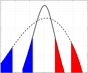
Figure 4 quantifies the probability density functions (p.d.f.s) of $B'_{q}$, with their skewness calculated by $S(B'_{q})=\langle B'^3_{q}\rangle /\langle B'^2_{q}\rangle ^{3/2}$ and annotated. In the $cold1$ case, the p.d.f. profile is slightly negatively skewed with $S(B'_{q})=-0.43$, even though this is hard to discern. As the wall-cooling intensity increases, this type of asymmetrical distribution becomes clear with the value of $S(B'_{q})$ decreasing to $-0.60$, and the extreme wall heat flux is intensified in the tails. As a consequence, the negative $B'_{q}$-events are stronger in intensity, but fewer in number than the positive ones. This phenomenon is consistent with the finding by Zhang et al. (2023) in the Mach number 8 case. (It is worth noting that the p.d.f. plot in their paper is in contrast to figure 4. This is because they defined $q_w$ analogous to wall shear stress in (3.1a,b) which is opposite to our definition $q_w = -K\partial T/\partial y|_w$.)

Figure 4. Probability density function of the wall-heat-flux fluctuations. The blue and red regions denote the extreme 2 % negative and positive $B'_{q}$-events.

The connection between $B'_{q}$ and the globally averaged Reynolds shear stress and turbulent heat flux is investigated, by means of ${\rm d} \langle -\rho u''v''\rangle ^*/{\rm d}B_q'$ and ${\rm d} \langle \rho v''\phi ''\rangle ^*/{\rm d}B_q'$, in figures 5 and 6. These $B_q'$-wise derivatives bear the advantage that their integrals with respect to $B'_{q}$ directly amount to the value of $-\langle \rho u''v''\rangle ^*$ and $\langle \rho v''\phi ''\rangle ^*$ at all wall-normal locations (Agostini & Leschziner 2019). Hence, they can quantify the contribution of $-\langle \rho u''v''\rangle ^*$ and $\langle \rho v''\phi ''\rangle ^*$ within a specific band of ${\rm d}B_q'$ to their respective total. From figure 5, the local quantity peaks mostly around $B_q'=0$, which is straightforwardly ascribed to the large population of $B'_{q}$-events there. Nevertheless, skewness to the positive events is observed in the map in figure 5(b) in the region $y^*<100$. Consistent with the wall-normal profile of $-\langle \rho u''v''\rangle ^*$, the magnitude of ${\rm d} \langle -\rho u''v''\rangle ^*/{\rm d}B_q'$ is small near the wall, with a significant percentage of it related to motions at the relatively large wall thermal perturbations. A similar phenomenon is found in the map of ${\rm d} \langle \rho v''\phi ''\rangle ^*/{\rm d}B_q'$ (in figure 6), with an exception that the contribution is mostly distributed in the outer region where the $B_q'$-wise derivatives exhibit approximate symmetry with regards to $B_q'= 0$ in both cases. However, as the population of events within a specific band of ${\rm d}B_q'$ varies with the intensity of fluctuations (see the p.d.f. in figure 4), the magnitude of $B_q'$-wise derivatives does not directly reflect the correlation of a single $B_q'$-event with the local properties. To this end, the variation of local mean quantities under the condition of $B_q'$ is investigated in the next section.

Figure 5. Map of the Reynolds-shear-stress derivative ${\rm d} \langle -\rho u''v''\rangle ^*/{\rm d}B_q'$ for cases (a) $cold1$ and (b) $cold2$.

Figure 6. Map of the turbulent-heat-flux derivative ${\rm d} \langle \rho v''\phi ''\rangle ^*/{\rm d}B_q'$ for cases (a) $cold1$ and (b) $cold2$.

4.3. Conditional sampling

The average of Reynolds shear stress and turbulent heat flux conditioned on the $B_q'$-events is further examined in this section. The conditional mean quantities, $-\langle \rho u'' v''\rangle ^*|_{B_q'}$ and $\langle \rho v''\phi ''\rangle ^*|_{B_q'}$, are expressed as

(4.1a)$$\begin{gather} -\langle \rho u'' v''\rangle ^*|_{B_q'} ={-}\langle \rho u v \rangle ^*|_{B_q'} +\langle \rho \rangle ^*|_{B_q'} \{ u \}^*|_{B_q'} \{v \}^*|_{B_q'}, \end{gather}$$

(4.1b)$$\begin{gather}\langle \rho v''\phi''\rangle ^*|_{B_q'} = \langle \rho v \phi \rangle ^*|_{B_q'}-\langle \rho\rangle ^*|_{B_q'} \{v\}^*|_{B_q'} \{\phi\}^*|_{B_q'}. \end{gather}$$

With (4.1a), the $-\langle \rho u'' v''\rangle ^*|_{B_q'}$ is quantified at all wall-normal locations in figure 7. Remarkable differences are observed between the left and right sides of the map in the near-wall region, indicating that positive and negative $B_q'$-events have distinct roles in the production of Reynolds shear stress. In particular, negative Reynolds shear stress is observed with negative $B_q'$-events close to the wall. Whereas further away from the wall, the connection between $-\langle \rho u'' v''\rangle ^*|_{B_q'}$ and ${B_q'}$ gradually weakens as $-\langle \rho u'' v''\rangle ^*|_{B_q'}$ barely changes with ${B_q'}$ at large wall-normal distances. An enhanced view of the distinctive properties is further shown in the profiles of the averaged Reynolds shear stress conditioned on the extreme 2 % negative and positive $B_q'$-events (blue and red regions in figure 4). In figure 7(c), in the near-wall region, the presence of positive wall-heat-flux perturbations is associated with the stronger generation of Reynolds shear stress when introducing additional heat into the fluid from the surface. In contrast, in the region $y^*>80$, the difference associated with the extreme positive and negative $B_q'$-events is almost indiscernible. This again confirms that the interaction between wall-heat-flux perturbations and Reynolds-shear-stress distribution is strong close to the wall, and is gradually attenuated further away from it (say, $y^*>80$ for cases under scrutiny).

Figure 7. (a,b) Map of the conditional average of Reynolds shear stress, $-\langle \rho u'' v''\rangle ^*|_{B_q'}$, for cases (a) $cold1$ and (b) $cold2$. (c) Profiles of the averaged Reynolds shear stress conditioned on the extreme 2 % negative and positive $B_q'$-events. The black solid lines in panels (a,b) denote the positive level, the black dashed lines denote the negative and the orange dashed line denotes 0.

To gain clearer insight into the correlation between ${B_q'}$ and the turbulent motions responsible for Reynolds shear stress, figure 8 plots the joint p.d.f.s of the fluctuations of streamwise and wall-normal velocities at a representative near-wall location, $y^*=8$, with respect to ${B_q'}$. It is observed that negative ${B_q'}$-events tend to be more closely associated with the positive $u''$-motions and more closely associated with the negative $v''$ in figure 8(a,b). This phenomenon is more evidently exhibited under the condition of stronger wall cooling in figure 8(d,e). Stronger ${B_q'}$ is in alignment with stronger turbulent dynamical motions. The extreme negative and positive ${B_q'}$-events are identified, to characterize their corresponding motions at the wall-normal location $y^*=8$. As shown in figure 8(c), under the condition of weaker wall cooling, the pre-multiplied joint p.d.f. of $u''/u_\infty$ and $v''/u_\infty$ conditioned on the overall $B_q'$-events (denoted by black solid lines) primarily manifests the strong sweep and ejection events in the near-wall cycle. The extreme 2 % positive ${B_q'}$-events (red lines) tend to be more correlated with ejections, whereas the extreme 2 % negative ${B_q'}$-events (blue lines) tend to be related to the sweep events. When the wall-cooling intensity increases, this trend is more pronouncedly presented, as seen in figure 8(f). In the self-sustaining cycle, the linear lift-up of streaks is associated with the even (varicose) instability mode, which is correlated with the wall-normal gradients of the streamwise velocity. However, the push-over of streaks is more connected to the odd (sinuous) mode, relying on the spanwise shear (Swearingen & Blackwelder 1987; Lozano-Durán et al. 2021). Hence, it suggests that the positive ${B_q'}$-events may correspond to the development of the even mode, which results in active transient growth of streamwise perturbations through a strong wall-normal shear of the inflectional streamwise velocity, while the negative ${B_q'}$-events may correspond to the development of the odd mode.

Figure 8. (a,d) Joint p.d.f. of $u''/u_\infty$ and $B_q'$, (b,e) joint p.d.f. of $v''/u_\infty$ and $B_q'$, and (c,f) pre-multiplied joint p.d.f. of $u''/u_\infty$ and $v''/u_\infty$, for cases (a,b,c) $cold1$ and (d,e,f) $cold2$ at $y^*=8$. The black solid lines in panels (a,b,d,e) represent the conditional averages of the global velocity perturbations, $\langle u''/u_\infty \rangle |_{B_q'}$ and $\langle v''/u_\infty \rangle |_{B_q'}$. The contours in panels (c,f) show fluctuations conditioned on the overall (black), extreme 2 % negative (blue) and extreme 2 % positive (red) $B_q'$-events.

The conditional average of turbulent heat flux, $\langle \rho v''\phi ''\rangle ^*|_{B_q'}$, is shown in figure 9. Similar to the observations in the distribution of the conditional average of Reynolds shear stress, the positive and negative ${B_q'}$-events play distinguishing roles in the distribution of turbulent heat flux. For instance, as shown in figure 9(a,b), the negative extreme ${B_q'}$ is in good alignment with the amplification of turbulent heat flux even in the region further away from the wall (e.g. at $y^*$ approximately 100), indicating that the negative wall events correspond to the enhanced thermodynamic perturbations there. This phenomenon is more straightforwardly displayed in the profiles of the averaged turbulent heat flux conditioned on the extreme 2 % negative and positive $B_q'$-events, as shown in figure 9(c). Differences between the contributions of positive and negative ${B_q'}$-events are clearly seen in the region even away from the wall, where the majority of thermal energy is produced (Fan & Li 2023). This is different from the finding in the map of $-\langle \rho u''v''\rangle ^*|_{B_q'}$, where the averaged quantities conditioned on the positive and negative extreme events almost converge for $y^*>80$, implying that the effect of wall temperature on the thermodynamic structures would be more outstretched in the wall-normal direction.

Figure 9. (a,b) Map of the conditional average of turbulent heat flux, $\langle \rho v'' \phi''\rangle ^*|_{B_q'}$, for cases (a) $cold1$ and (b) $cold2$. (c) Profiles of the averaged turbulent heat flux conditioned on the extreme 2 % negative and positive $B_q'$-events.

In a similar manner, figure 10 delineates the joint p.d.f.s of the velocities and wall-heat-flux perturbations at $y^*=8$, to reveal the correlation between the dynamical motion and thermal quantity. In both cases, $B_q'$ is slightly negatively correlated with $\phi ''$, while positively correlated with $v''$ at the selected height (shown by the black solid lines in figure 10a,b,d,e). It thus leads to differences in the $\phi ''$–$v''$ correlations conditioned on the overall, extreme 2 % negative and positive $B_q'$-events. In the $cold1$ case, in figure 10(c), a relatively larger population is seen in Quarter 1 (where $\phi ''>0$ and $v''>0$) and Quarter 3 (where $\phi ''<0$ and $v''<0$), indicating that $\phi ''$ and $v''$ are mostly positively correlated with each other yielding positive turbulent heat flux, as shown in figures 2(d) and 9(c). Nevertheless, a negative correlation of $\phi ''$ and $v''$ appears, with the negative $B_q'$-events preferring the downward motions while the positive ones preferring the upward motions. When there is stronger heat flux at the wall (see figure 10f), the situation differs in that events are more evidently scattered in Quarter 2 (where $\phi ''<0$ and $v''>0$) and Quarter 4 (where $\phi ''>0$ and $v''<0$). This is associated with the sign reversal of temperature gradient within the turbulent boundary layer. At $y^*=8$, the positive thermal structures tend to be carried towards the lower-temperature (lower) layers and the negative thermal structures to the higher-temperature (upper) layers (Pirozzoli & Bernardini 2011; Fan, Li & Sandberg 2023). The positive $v''$ motions conditioned on the positive $B_q'$-events are again accentuated in figure 10(f), indicating that the receipt of heat flux from the wall preferentially corresponds to the lift-up of turbulent motions.

Figure 10. (a,d) Joint p.d.f. of $\phi ''/\phi _\infty$ and $B_q'$, (b,e) joint p.d.f. of $v''/u_\infty$ and $B_q'$, and (c,f) pre-multiplied joint p.d.f. of $\phi ''/\phi _\infty$ and $v''/u_\infty$, for cases (a,b,c) $cold1$ and (d,e,f) $cold2$ at the wall-normal location $y^*=8$. The black solid lines in panels (a,d) track the conditional average $\langle \phi ''/\phi _\infty \rangle |_{B_q'}$.

4.4. The correlation between $B_q'$ and the transport budgets

The Reynolds shear stress and turbulent heat flux evolve in space. To elucidate the interaction of wall heat flux and the evolution process, budgets in the transport equations for Reynolds shear stress and turbulent heat flux are examined in detail.

4.4.1. Evolution of Reynolds shear stress

Figure 11 shows the one-dimensional profiles of the budget terms from (2.1) in semilocal units, as a function of $y^*$. The budget variables are normalized by $\langle \rho \rangle u_\tau ^{*3}/\delta _\nu ^*$. The term of mass contribution associated with the density variation, i.e. $M_{-\rho u v}^*$, is neglected due to its relatively trivial magnitude for the present cases. Figure 11 shows that the Reynolds shear stress is largely produced in the inner region ($\kern0.7pt y^*<50$), with the peak of the production term ($P_{-\rho uv}^*$) located at $y^*\approx 17$ for both cases. The correlation between velocity and pressure gradient, denoted by $\varPhi _{-\rho uv}^{p*}= D_{-\rho uv}^{p*}+\varPi _{-\rho uv}^{p*}$, yields negative results, and plays a significant role in diffusing the Reynolds shear stress in space and exchanging it among components (Lee & Moser 2019). Regardless of the wall thermal condition, the semilocal scaling is able to well collapse the inner peak location of $\varPhi _{-\rho uv}^{p*}$, preventing the wall-normal shift in classical inner units (Zhang et al. 2018; Cogo et al. 2023). The imbalance between $P_{-\rho uv}^*$ and $\varPhi _{-\rho uv}^{p*}$ is consequently compensated for by turbulent diffusion ($D_{-\rho uv}^{t*}$) and viscous action ($\varPhi _{-\rho uv}^{\nu *}= D_{-\rho uv}^{\nu *}-\varepsilon _{-\rho uv}^{*}$), with the turbulent diffusion mildly larger in peak magnitude in both cases. When the wall cooling is intensified, a negative peak of $D_{-\rho uv}^{t*}$ appears in a region very close to the wall (e.g. $y^*\approx 4$, see figure 11b), which is probably associated with the stronger conduction of heat in this region. In the following discussion, attention will be paid to the major process of production ($P_{-\rho uv}^*$), pressure work ($\varPhi _{-\rho uv}^{p*}$) and turbulent diffusion ($D_{-\rho uv}^{t*}$), and their connection with the wall-heat-flux-perturbation events.

Figure 11. Profiles of budget terms in the transport equation for Reynolds shear stress, normalized with semilocal units, for cases (a) $cold1$ and (b) $cold2$. Here, $\varPhi _{-\rho uv}^{\nu *} = D_{-\rho uv}^{\nu *}-\varepsilon _{-\rho uv}^*$ represents the viscous action and $\varPhi _{-\rho uv}^{p*} = D_{-\rho uv}^{p*}+\varPi _{-\rho uv}^{p*}$ denotes the velocity-pressure-gradient correlation.

Figures 12(a) and 12(b) show the conditional average of pre-multiplied Reynolds-shear-stress production, under the two different wall-cooling conditions. A similar phenomenon is seen in both cases, that stronger $B_q'$-events are correlated with a more noticeable Reynolds shear stress generation, particularly when the instantaneous heat-flux perturbations at the wall are positive. This is consistent with the observations in figure 7, and can be more straightforwardly displayed by the conditionally averaged quantities based on the extreme events in figure 12(c). The difference between the roles of extreme positive and negative $B_q'$-events is found mainly in the inner-layer cycle. The production of Reynolds shear stress is more strongly correlated with the positive extreme events, except in the region $y^*<10$ in the $cold2$ case. To identify the underlying flow characteristics, the two predominant terms that contribute to $P_{-\rho uv}^*$, namely the wall-normal Reynolds stress ($\langle \rho v''v''\rangle ^*$) and the gradient of streamwise velocity (${\rm d}\{u\}^*/{\rm d} y^*$) according to (2.2a), are investigated in the wall-normal coordinate. To make it consistent with the scaling of budgets in figure 11, the velocity gradient (${\rm d}\{u\}^*/{\rm d} y^*$) is semilocally scaled by $u_\tau ^*/\delta _\nu ^*$. Figure 13 plots the profiles of the $\langle \rho v''v''\rangle ^*|_{B_q'}$ and ${\rm d}\{u\}^*/{\rm d} y^*|_{B_q'}$ conditioned on the extreme 2 % negative and positive $B_q'$-events, respectively, for both cases. It is observed that in the region $y^*<500$ for the $cold1$ case and $y^*<200$ for the $cold2$ case, the wall-normal Reynolds stress is weakened in the presence of positive $B_q'$-events, indicating that instantaneous wall heating ($B_q'>0$) corresponds to the attenuated wall-normal fluid motions. Beyond that, the positive and negative curves almost collapse onto each other. The plot of ${\rm d}\{u\}^*/{\rm d} y^*|_{B_q'}$ in figure 13(b) demonstrates that under the condition of positive $B_q'$-events, the mean velocity gradient is diminished near the wall, whereas it is enhanced in the layer $10< y^*<100$ in contrast to the negative $B_q'$-events. In this sense, it suggests that the increment of $P_{-\rho uv}^*$ in this region is shear-induced under the condition of positive extreme events.

Figure 12. (a,b) Map of the conditional average of pre-multiplied Reynolds-shear-stress production, $y^*P_{-\rho uv}^*|_{B_q'}$, for cases (a) $cold1$ and (b) $cold2$. (c) Profiles of the averaged pre-multiplied production conditioned on the extreme 2 % negative and positive $B_q'$-events.

Figure 13. Profiles of (a) the averaged wall-normal Reynolds stress and (b) the gradient of the Favre averaged streamwise velocity, conditioned on the extreme 2 % negative and positive $B_q'$-events.

The conditional average of pre-multiplied velocity-pressure-gradient is examined in figure 14(a,b). Similar to the findings for production, stronger $B_q'$-events tend to correspond to a stronger physical process of pressure work. For both $cold1$ and $cold2$ cases, positive/negative $B_q'$-events are tendentiously in alignment with negative/positive $\varPhi _{-\rho uv}^{p*}$ close to the wall. The sign reverses along the wall-normal direction, with different distributions under the condition of various $B_q'$-events. As is more clearly shown in the profiles of $y^*\varPhi _{-\rho uv}^{p*}$ conditioned on the extreme events in figure 14(c), the negative $\varPhi _{-\rho uv}^{p*}$ appears in a region nearer to the wall in the presence of positive thermal events than negative events.

Figure 14. (a,b) Map of the conditional average of pre-multiplied velocity-pressure-gradient correlation, $y^*\varPhi _{-\rho uv}^{p*}|_{B_q'}$, for cases (a) $cold1$ and (b) $cold2$. (c) Profiles of the averaged $y^*\varPhi _{-\rho uv}^{p*}$ conditioned on the extreme 2 % negative and positive $B_q'$-events.

For the conditional average of pre-multiplied turbulent diffusion, as mapped in figure 15(a), the $B_q'$ is in slight association with the distribution of turbulent diffusion in the $cold1$ case, as manifested by the almost collapsed contribution of extreme negative and positive events in figure 15(c). With stronger wall cooling, as presented in figure 15(b), the negative $B_q'$-events tend to be related to the amplified diffusion process near the wall, leading to a net transport of Reynolds stress from this region to other regions. Further away from the wall, the intercorrelation of the turbulent diffusion and the $B_q'$-events is weakened progressively.

Figure 15. (a,b) Map of the conditional average of pre-multiplied turbulent diffusion of Reynolds shear stress, $y^*D_{-\rho uv}^{t*}|_{B_q'}$, for cases (a) $cold1$ and (b) $cold2$. (c) Profiles of the averaged $y^*D_{-\rho uv}^{t*}$ conditioned on the extreme 2 % negative and positive $B_q'$-events.

4.4.2. Evolution of turbulent heat flux

The wall-normal distributions of the budget terms in (2.4) are depicted in figure 16. The contribution of density and temperature variation to the turbulent-heat-flux evolution, $M_{\rho v \phi }^*$, is excluded due to its relatively small magnitude compared with the other terms, for the cases under scrutiny. In a similar manner to the transport of Reynolds shear stress, the production of $\langle \rho v'' \phi '' \rangle ^*$ is majorly expended in pressure work. The turbulent motions, viscous action and heat conduction serve to transport thermal energy across the boundary layer so as to ensure the balance of the system. A particularly interesting feature is observed in the $cold2$ case, that the production term ($P_{\rho v\phi }^*$) is negative in the region beneath $y^*\approx 10$, where the mean temperature exhibits a maximum. This is consistent with the near-wall profile of $\langle \rho v'' \phi '' \rangle ^*$ in figure 2(d), as the wall-normal motions from higher-temperature to lower-temperature regions always communicate positive $\phi$ fluctuations (Pirozzoli & Bernardini 2011). Consequently, heat conduction is enhanced via stronger wall cooling and plays a considerable role in redistributing the thermal energy especially in $y^*<5$. To reveal the correlation of $\langle \rho v'' \phi '' \rangle ^*$ transport and the fluctuation events of wall heat flux, conditional averages of production ($P_{\rho v\phi }^*$), pressure work ($W_{\rho v\phi }^{p*}$) and turbulent diffusion ($D_{\rho v\phi }^{t*}$) on $B_q'$-events are of major interest.

Figure 16. Profiles of budget terms in the transport equation for turbulent heat flux, normalized with semilocal units, for cases (a) $cold1$ and (b) $cold2$.

Figure 17 plots the conditional average of $y^*P_{\rho v\phi }^*$, showing that the interaction of $B_q'$ and production exists mainly at $y^*<200$. The larger generation of turbulent heat flux tends to be preferentially in correspondence with the negative events, in most of this region. This is partly owing to the stronger wall-normal motions under the condition of instantaneous wall cooling ($B_q'<0$, seen in figure 13), as the wall-normal Reynolds stress is one of the main contributing factors to production formulated in (2.5a). An exception occurs in the viscous sublayer in the $cold2$ case. For $y^*<4$, the profile of $y^*P_{\rho v\phi }^*$ conditioned on the extreme 2 % negative $B_q'$-events is slightly lower than that conditioned on the positive events, as shown by the red and blue dashed lines in figure 17(c). To explain this phenomenon, profiles of another contributing factor $\{\phi \}/\phi _w$ and its wall-normal gradient ${\rm d}\{\phi \}^*/{\rm d} y^*$, conditioned on the extreme 2 % $B_q'$-events, are shown in figure 18. Herein, ${\rm d}\{\phi \}^*/{\rm d} y^*$ denotes the gradient normalized by $u_\tau ^*/\delta _\nu ^*$. For both cases, it is observed that the extreme negative events correspond to a higher local temperature, which is proportional to $\phi ^2$, for $y^*<500$ for the case $cold1$ and $y^*<15$ for $cold2$. Hence, the temperature variation (gradient) is relatively faster (larger) close to the wall, in the presence of negative $B_q'$-events than positive $B_q'$-events, as shown in figure 18(b), leading to a larger production in absolute magnitude which amounts to the smaller negative $y^*P_{\rho v\phi }^*$ delineated by the blue dashed curve in figure 17(c).

Figure 17. (a,b) Map of the conditional average of pre-multiplied turbulent-heat-flux production, $y^*P_{\rho v\phi }^*|_{B_q'}$, for cases (a) $cold1$ and (b) $cold2$. (c) Profiles of the averaged $y^*P_{\rho v\phi }^*$ conditioned on the extreme 2 % negative and positive $B_q'$-events. The black dashed line in panel (c) denotes 0.

Figure 18. Profiles of (a) $\{\phi \}/\phi _w$ and (b) the gradient ${\rm d}\{\phi \}^*/{\rm d} y^*$, conditioned on the extreme 2 % negative and positive $B_q'$-events.

As for the correlation of wall-heat-flux fluctuations and the contribution of pressure work in the transport of turbulent heat flux across the boundary layer, the conditionally averaged distribution of $y^*W_{\rho v\phi }^{p*}$ is given in figure 19. In general, in the context of the extreme $B_q'$-events, the pressure work is enhanced in an inner region $y^*<100$, but with different phenomena observed in the two cases. As shown in figure 19(c), for the case $cold1$, the absolute magnitude of $y^* W_{\rho v\phi }^{p*}$ conditioned on the negative events is amplified in most regions, which is mainly ascribed to the sound-speed-pressure-gradient correlation, i.e. the second term on the right-hand side of (2.5c) (the decomposed plots are not shown for brevity). Conversely, for the $cold2$ case, the bias to the contribution of extreme negative or positive events is not evident throughout the boundary layer.

Figure 19. (a,b) Map of the conditional average of pre-multiplied pressure work, $y^*W_{\rho v\phi }^{p*}|_{B_q'}$, for cases (a) $cold1$ and (b) $cold2$. (c) Profiles of the averaged $y^* W_{\rho v\phi }^{p*}$ conditioned on the extreme 2 % negative and positive $B_q'$-events.

At last, an approximate symmetry of $y^*D_{\rho v\phi }^{t*}|_{B_q'}$ with regards to $B_q'=0$ is observed in figure 20(a), suggesting that the turbulent diffusion of turbulent heat flux is not sensitive to the fluctuations of wall heat flux with a weaker wall cooling. The profiles of the averaged $y^*D_{-\rho v\phi }^{t*}$ conditioned on the extreme negative and positive $B_q'$-events almost collapse (solid lines in figure 20c). This is similar to the finding in the turbulent diffusion of Reynolds shear stress. As for the case $cold2$, the turbulent diffusion associated with the negative events is enhanced near the wall in figure 20(b), and tends to converge to that under the condition of positive events away from the wall.

Figure 20. (a,b) Map of the conditional average of pre-multiplied turbulent diffusion of turbulent heat flux, $y^*D_{-\rho v\phi }^{t*}|_{B_q'}$, for cases (a) $cold1$ and (b) $cold2$. (c) Profiles of the averaged $y^*D_{-\rho v\phi }^{t*}$ conditioned on the extreme 2 % negative and positive $B_q'$-events.

5. Conclusions

The correlation between the mean and fluctuating wall heat flux and the distribution and transport of Reynolds shear stress/turbulent heat flux is thoroughly investigated in this study. Transport equations are derived rigorously incorporating a sound-speed-like variable ($\phi \propto c$), following the previous study on the framework of energy exchange in compressible turbulent flows. Using the DNS databases of two hypersonic boundary layers under the condition of a weaker ($cold1$) and stronger ($cold2$) wall cooling, we examine the characteristics of wall-heat-flux perturbations ($B_q'$) through their instantaneous field and p.d.f. plot. With the increasing wall-cooling intensity, the extreme $B_q'$-events become more intense and the p.d.f. profile of $B_q'$ tends to exhibit a negatively skewed distribution, which results in stronger negative $B'_{q}$-events in intensity but fewer in number.

In the presence of positive $B_q'$-events, Reynolds shear stress is increased in the near-wall region of both cases under scrutiny. Through the joint p.d.f.s of velocities and the wall-heat-flux perturbations, $B_q'$ is found to have a predominantly negative correlation with $u''$ and a positive correlation with $v''$ at $y^*=8$. Stronger perturbations in wall heat flux are associated with stronger dynamical motions. As a consequence, the extreme negative $B_q'$-events tend to be more correlated to the sweep events, as is especially observed in the stronger wall-cooling case, whereas the extreme positive events are correlated with ejections. However, negative $B_q'$-events are in good alignment with the amplification of turbulent heat flux even in the region further away from the wall, suggesting that the effect of wall temperature on the thermodynamic structures would be extended in the wall-normal direction. Negative turbulent heat flux emerges near the wall, with a different underlying mechanism under the condition of positive and negative $B_q'$-events. In this case, negative $B_q'$-events prefer positive $\phi ''$ and negative $v''$ (downward motions), and vice versa.

Finally, in the transport of Reynolds shear stress and turbulent heat flux, production is primarily balanced by pressure work and turbulent diffusion. Conditional analysis reveals that the instantaneous wall heating ($B_q'>0$) is in alignment with the larger production of Reynolds shear stress which is induced by the enlarged shear, in contrast to the instantaneous wall cooling ($B_q'<0$). However, the positive $B_q'$ corresponds to a smaller production of turbulent heat flux primarily associated with the attenuation of wall-normal fluid motions. An exception is found in the viscous sublayer in the $cold2$ case, where the relatively slower temperature variation close to the wall causes a comparatively larger negative production of turbulent heat flux when $B_q'>0$.

References

Agostini, L. & Leschziner, M. 2019 The connection between the spectrum of turbulent scales and the skin-friction statistics in channel flow at ${Re}_\tau \approx 1000$. J. Fluid Mech. 871, 2251.CrossRefGoogle Scholar
Bernardini, M., Modesti, D., Salvadore, F. & Pirozzoli, S. 2021 STREAmS: a high-fidelity accelerated solver for direct numerical simulation of compressible turbulent flows. Comput. Phys. Commun. 263, 107906.CrossRefGoogle Scholar
Cogo, M., Baù, U., Chinappi, M., Bernardini, M. & Picano, F. 2023 Assessment of heat transfer and Mach number effects on high-speed turbulent boundary layers. J. Fluid Mech. 974, A10.CrossRefGoogle Scholar
Cogo, M., Salvadore, F., Picano, F. & Bernardini, M. 2022 Direct numerical simulation of supersonic and hypersonic turbulent boundary layers at moderate-high Reynolds numbers and isothermal wall condition. J. Fluid Mech. 945, A30.CrossRefGoogle Scholar
Dong, S.-W., Tong, F.-L., Yu, M., Chen, J.-Q., Yuan, X.-X. & Wang, Q. 2022 Positive and negative pairs of fluctuating wall shear stress and heat flux in supersonic turbulent boundary layers. Phys. Fluids 34 (8), 085115.CrossRefGoogle Scholar
Duan, L., Beekman, I. & Martin, M.P. 2010 Direct numerical simulation of hypersonic turbulent boundary layers. Part 2. Effect of wall temperature. J. Fluid Mech. 655, 419445.CrossRefGoogle Scholar
Fan, Y.-T. & Li, W.-P. 2023 Spectral analysis of turbulence kinetic and internal energy budgets in hypersonic turbulent boundary layers. Phys. Rev. Fluids 8, 044604.CrossRefGoogle Scholar
Fan, Y.-T., Li, W.-P. & Pirozzoli, S. 2022 Energy exchanges in hypersonic flows. Phys. Rev. Fluids 7, L092601.CrossRefGoogle Scholar
Fan, Y.-T., Li, W.-P. & Sandberg, R.D. 2023 Resolvent-based analysis of hypersonic turbulent boundary layers with/without wall cooling. Phys. Fluids 35 (4), 045118.Google Scholar
Griffin, K.P., Fu, L. & Moin, P. 2021 Velocity transformation for compressible wall-bounded turbulent flows with and without heat transfer. Proc. Natl Acad. Sci. 118 (34), e2111144118.CrossRefGoogle ScholarPubMed
Hasan, A.M., Larsson, J., Pirozzoli, S. & Pecnik, R. 2023 Incorporating intrinsic compressibility effects in velocity transformations for wall-bounded turbulent flows. Phys. Rev. Fluids 8, L112601.CrossRefGoogle Scholar
Huang, J., Duan, L. & Choudhari, M.M. 2022 Direct numerical simulation of hypersonic turbulent boundary layers: effect of spatial evolution and Reynolds number. J. Fluid Mech. 937, A3.CrossRefGoogle Scholar
Huang, P.G., Coleman, G.N. & Bradshaw, P. 1995 Compressible turbulent channel flows: DNS results and modelling. J. Fluid Mech. 305, 185218.CrossRefGoogle Scholar
Huang, P.G., Coleman, G.N., Spalart, P.R. & Yang, X.I.A. 2023 Velocity and temperature scalings leading to compressible laws of the wall. J. Fluid Mech. 977, A49.CrossRefGoogle Scholar
Kawata, T. & Alfredsson, P.H. 2018 Inverse interscale transport of the Reynolds shear stress in plane Couette turbulence. Phys. Rev. Lett. 120, 244501.CrossRefGoogle ScholarPubMed
Kawata, T. & Tsukahara, T. 2022 Spectral analysis on transport budgets of turbulent heat fluxes in plane Couette turbulence. Energies 15 (14), 5258.CrossRefGoogle Scholar
Kim, J. & Moin, P. 1989 Transport of passive scalars in a turbulent channel flow. In Turbulent Shear Flows 6 (ed. J.C. André, J. Cousteix, F. Durst, B.E. Launder, F.W. Schmidt & J.H. Whitelaw), pp. 85–96. Springer.CrossRefGoogle Scholar
Lee, M.-K. & Moser, R.D. 2019 Spectral analysis of the budget equation in turbulent channel flows at high Reynolds number. J. Fluid Mech. 860, 886938.CrossRefGoogle Scholar
Lele, S.K. 1994 Compressibility effects on turbulence. Annu. Rev. Fluid Mech. 26 (1), 211254.CrossRefGoogle Scholar
Liang, X. & Li, X.-L. 2015 Direct numerical simulation on Mach number and wall temperature effects in the turbulent flows of flat-plate boundary layer. Commun. Comput. Phys. 17 (1), 189212.CrossRefGoogle Scholar
Lozano-Durán, A., Constantinou, N.C., Nikolaidis, M.-A. & Karp, M. 2021 Cause-and-effect of linear mechanisms sustaining wall turbulence. J. Fluid Mech. 914, A8.CrossRefGoogle Scholar
Mittal, A. & Girimaji, S.S. 2019 Mathematical framework for analysis of internal energy dynamics and spectral distribution in compressible turbulent flows. Phys. Rev. Fluids 4, 042601.CrossRefGoogle Scholar
Miura, H. & Kida, S. 1995 Acoustic energy exchange in compressible turbulence. Phys. Fluids 7, 1732.CrossRefGoogle Scholar
Patel, A., Peeters, J.W.R., Boersma, B.J. & Pecnik, R. 2015 Semi-local scaling and turbulence modulation in variable property turbulent channel flows. Phys. Fluids 27 (9), 185218.CrossRefGoogle Scholar
Pirozzoli, S. & Bernardini, M. 2011 Turbulence in supersonic boundary layers at moderate Reynolds number. J. Fluid Mech. 688, 120168.CrossRefGoogle Scholar
Praturi, D.S. & Girimaji, S.S. 2019 Effect of pressure-dilatation on energy spectrum evolution in compressible turbulence. Phys. Fluids 31 (5), 055114.CrossRefGoogle Scholar
Shadloo, M.S., Hadjadj, A. & Hussain, F. 2015 Statistical behavior of supersonic turbulent boundary layers with heat transfer at ${M}_\infty = 2$. Intl J. Heat Fluid Flow 53, 113134.CrossRefGoogle Scholar
Swearingen, J.D. & Blackwelder, R.F. 1987 The growth and breakdown of streamwise vortices in the presence of a wall. J. Fluid Mech. 182, 255290.CrossRefGoogle Scholar
Tong, F.-L., Dong, S.-W., Lai, J., Yuan, X.-X. & Li, X.-L. 2022 Wall shear stress and wall heat flux in a supersonic turbulent boundary layer. Phys. Fluids 34 (1), 015127.CrossRefGoogle Scholar
Wenzel, C., Gibis, T. & Kloker, M. 2022 About the influences of compressibility, heat transfer and pressure gradients in compressible turbulent boundary layers. J. Fluid Mech. 930, A1.CrossRefGoogle Scholar
Xu, D.-H., Wang, J.-C., Wan, M.-P., Yu, C.-P., Li, X.-L. & Chen, S.-Y. 2021 a Compressibility effect in hypersonic boundary layer with isothermal wall condition. Phys. Rev. Fluids 6, 054609.CrossRefGoogle Scholar
Xu, D.-H., Wang, J.-C., Wan, M.-P., Yu, C.-P., Li, X.-L. & Chen, S.-Y. 2021 b Effect of wall temperature on the kinetic energy transfer in a hypersonic turbulent boundary layer. J. Fluid Mech. 929, A33.CrossRefGoogle Scholar
Yu, M. & Xu, C.-X. 2021 Compressibility effects on hypersonic turbulent channel flow with cold walls. Phys. Fluids 33 (7), 075106.CrossRefGoogle Scholar
Zhang, C., Duan, L. & Choudhari, M.M. 2018 Direct numerical simulation database for supersonic and hypersonic turbulent boundary layers. AIAA J. 56 (11), 42974311.CrossRefGoogle Scholar
Zhang, P.-J.-Y., Wan, Z.-H., Dong, S.-W., Liu, N.-S., Sun, D.-J. & Lu, X.-Y. 2023 Conditional analysis on extreme wall shear stress and heat flux events in compressible turbulent boundary layers. J. Fluid Mech. 974, A38.CrossRefGoogle Scholar
Zhang, Y.-S., Bi, W.-T., Hussain, F. & She, Z.-S. 2014 A generalized reynolds analogy for compressible wall-bounded turbulent flows. J. Fluid Mech. 739, 392420.CrossRefGoogle Scholar