Near-tip correction functions for the actuator line method to improve the predicted lift and drag distributions

Abstract

The actuator line method (ALM) is a commonly used technique to simulate slender lifting and dragging bodies such as wings or blades. However, the accuracy of the method is significantly reduced near the tip. To quantify the loss of accuracy, translating wings with various aspect and taper ratios are simulated using several methods: wall-resolved Reynolds-averaged Navier–Stokes (RANS) simulations, an advanced ALM with two-dimensional (2-D) mollification of the force, a lifting line method, a mollified lifting line method and a vortex lattice method. Significant differences in the lift and drag distributions are found on the part of the wing where the distance to the tip is smaller than approximately 3 chords and are identified to arise from both the forces mollification and the uneven induced velocity along the chord. Correction functions acting on the lift coefficient and effective angle of attack near the wing tip are then derived for rectangular wings of various aspect ratios. They are then also applied to wings of various taper ratios using the ‘effective dimensionless distance to the tip’ as the main parameter. The application of the correction not only leads to a much improved lift distribution, but also to a more consistent drag distribution. The correction functions are also obtained for various mollification sizes, as well as for ALM with three-dimensional (3-D) mollification. These changes mostly impact the correction for the effective angle of attack. Finally, the correction is applied to simulations of the NREL Phase VI wind turbine, leading to an enhanced agreement with the experimental data.

1. Introduction

The actuator line method (ALM), introduced by Sorensen & Shen (2002), is a technique that allows for performing numerical simulations of slender lifting and dragging bodies. It consists of adding a source term to the Navier–Stokes equations to model the influence of the aerodynamic forces on the flow. The aerodynamic forces are computed using the measured local flow velocity and the lift and drag coefficients of the section aerodynamic profile obtained using its polar. The computational cost of numerical simulations is considerably less compared with that of body-resolved simulations. This method received significant attention, especially in the wind energy sector where it has been extensively used to perform large eddy simulation (LES) of the wake developing behind horizontal axis wind turbines (Breton et al. 2017). More recently, its usage has also been extended to various other applications, including vertical axis wind turbines, propellers, rotors of helicopters or translating wings (see e.g. Shamsoddin & Porté-Agel 2014; Bühler et al. 2018; Mendoza et al. 2018; Stokkermans et al. 2019; Melani et al. 2021; Merabet & Laurendeau 2022; Kleine, Hanifi & Henningson 2023b).

However, the accuracy of the ALM decreases near the tip for two main reasons: the mollification of the forces (Caprace, Chatelain & Winckelmans 2019) and the uneven induced velocity along the airfoil chord (Sørensen, Dag & Ramos-García 2016). Indeed, the ALM requires to use a mollification of the aerodynamic force evaluated on each section to distribute it over the nearby grid points of the flow solver. This step is required to ensure numerical stability by avoiding the addition of a singular force in the simulation. Typically, the forces computed on the actuator line are regularized by convoluting them with a Gaussian kernel, which significantly affects the vorticity field in the near wake. This results in a decrease of the induced velocity as measured on the aerodynamic centreline, leading to higher effective angles of attack and therefore higher aerodynamics loads. Additionally, the flow near the wing/blade tip presents a three-dimensional (3-D) behaviour that is not taken into account in the ALM. This includes the variation of the induced velocity along the chord of the airfoil, known as the ‘virtual camber effect’ (Sørensen et al. 2016). Indeed, the region of the airfoil near the trailing edge is deeper in the wake than the leading edge, and therefore undergoes a larger downwash. As a result, the streamline along the chord is curved, which can be considered as an additional camber of the airfoil. This ‘virtual camber’ modifies the aerodynamic properties of the airfoil and causes a variation of the loads, especially near the tip where the induced velocity is consequent. In the ALM, the velocity is only sampled at the quarter chord position, and hence does not account for the uneven downwash, resulting in an over-prediction of the loads. Some strategies have been developed to mitigate these effects and improve the accuracy of the ALM. These strategies include modifying the mollification or applying tip corrections, as described below.

The ALM can be improved by using more accurate mollification kernels. The original ALM is regularized using an isotropic 3-D Gaussian kernel with a constant width $\sigma$ along the blade (Sorensen & Shen 2002). The value of $\sigma$ is constrained by numerical stability, which typically requires $\sigma \ge 2h$, where $h$ is the grid spacing (Troldborg 2008). The size of the kernel width is often chosen relatively to the airfoil chord. For instance, Martínez-Tossas, Churchfield & Meneveau (2017) showed that a kernel size of $\sigma \simeq c/4$ minimizes the difference between the flow field induced by a regularized Gaussian vortex and the potential flow past an airfoil. The possibility of varying the kernel width along the span was also investigated. Jha et al. (2014) scaled the kernel width with the local chord of the blade, or with an equivalent elliptic chord distribution. It was found that using the elliptic chord distribution increases the accuracy at the blade tip, since it reduces the mollification in the critical tip region. Anisotropic kernels were also used by Churchfield et al. (2017) to modify the mollification width according to the airfoil direction. A significant improvement of the accuracy of the loads at the tip and of the near wake was found when the force distribution matched the shape of the airfoil. It was then identified that the spanwise mollification is detrimental to the accuracy because it distributes the force beyond the blade tip. Some research has therefore been conducted using a two-dimensional (2-D) mollification in the plane of the airfoil (Mikkelsen 2004; Shives & Crawford 2013; Jha & Schmitz 2018). The absence of mollification in the spanwise direction indeed led to a noticeable improvement of the blade tip behaviour compared with the 3-D kernel.

Tip corrections can also be used to improve the accuracy of the loads. The correction developed by Glauert (1935) for the blade element momentum (BEM) theory has been used by some authors for their ALM applied to wind turbines (Martinez et al. 2012; Jha et al. 2014); nevertheless, such usage should not be necessary as an ALM represents the individual blades that each shed their own vortex wake which is captured by the LES flow solver. Additionally, the correction of Glauert for the BEM is a modification of Prandtl's tip-loss factor that was initially developed for lightly loaded rotors. It does not account for the wake expansion, roll-up and distortion, which were shown to influence the tip correction (Branlard, Dixon & Gaunaa 2013). Extension of the tip-loss factor has therefore also been obtained for BEM by Branlard et al. (2013) and Maniaci & Schmitz (2016). Shen et al. (2005a) and Shen, Sørensen & Mikkelsen (2005b) later introduced an empirical correction similar to that of Glauert to account for 3-D flow effects at the tip. In fact, he underlined that the force at the tip should be zero due to pressure equalization, even if the flow angle is in general not zero. He therefore suggested a modification of the 2-D lift and drag coefficient to enforce zero force in the near-tip region. This correction was then extended by Wimshurst & Willden (2017) by comparing ALM to blade-resolved simulations and deriving separate correction functions for the normal and tangential loads. Pirrung et al. (2020) then showed that applying the Shen correction to the angle of attack led to an improved accuracy of the normal and tangential loads. Sørensen et al. (2016) also developed a decambering correction to take into account the variation of the induced velocity on the blade surface when using a lifting line approach. Indeed, the induced velocity varies along the airfoil due to the fact that the trailing edge is deeper in the wake than the leading edge. By combining the lifting line theory with the thin airfoil theory, an analytical correction was developed for the distribution of the circulation on wings with moderate aspect ratios.

More recently, new smearing corrections were developed to remove the spurious effects of the forces mollification. Meyer Forsting, Pirrung & Ramos-García (2019) and Dag & Sørensen (2020) developed a method to correct the induced velocity on the line by comparing the velocity induced by a regularized vorticity field with that of a singular one. This correction requires to use a vortex model of the near wake that runs concurrently with the ALM simulation. The model provides the value of the missing induction, which is used to re-estimate the circulation iteratively. Kleine, Hanifi & Henningson (2023a) then linearized this problem to obtain a non-iterative correction. Martínez-Tossas & Meneveau (2019) used a filtered lifting theory to correct the induced velocity on an ALM with an arbitrary mollification width to the value that would be obtained using the optimal width $\sigma \simeq c/4$. Stanly et al. (2022) applied this correction to the case of horizontal wind turbines, leading to an improved loading at the blade tip and a better agreement with experimental data.

Whereas it is commonly admitted that the ALM overpredicts the loads at the tip, it remains difficult to quantify the effects and relative importance of the mollification and of the virtual camber on a given wing. In fact, the studies that consider the effect of the mollification typically evaluate the effect of the correction using comparison with the lifting line (Meyer Forsting et al. 2019; Dag & Sørensen 2020; Kleine et al. 2023a) or the blade element momentum theory (Jha et al. 2014; Dag & Sørensen 2020), or comparing various mollification sizes (Martínez-Tossas & Meneveau 2019). This approach does not allow one to compare the effect of the mollification with that of the virtual camber effect. Melani, Balduzzi & Bianchini (2022) performed a comparison of both a fixed and rotating wing between ALM and wall-resolved Reynolds-averaged Navier–Stokes (RANS) simulations, and found that, although the correction was beneficial for the accuracy, the lift obtained using wall-resolved RANS simulations still differed from the ALM on the last 20 % of the blade, likely due to the virtual camber. Moreover, the corrections that require the use of a free-vortex wake model are not straightforward to apply, and increase the computational cost of the force evaluation. In addition, the aforementioned corrections are designed to act on the lift distribution, but their effect on the drag distribution is not assessed. This can be problematic for applications in which the drag plays a significant role, such as the evaluation of the performances of wind turbines.

In this paper, a thorough analysis of translating wings is first conducted using various aerodynamic methods. The lift and drag distributions obtained using high-fidelity wall-resolved simulations are compared with those predicted by the ALM and other simplified models: the Prandtl lifting line theory, its mollified version (Caprace et al. 2019) and the vortex lattice method (Katz & Plotkin 2001). This allows us to confirm that the impact of the mollification and of the virtual camber are the two main sources of differences between the ALM and the reference results; at least as far as the lift is concerned. The impact on the drag components (induced drag and parasitic drag) is more complex to assess, and is here also investigated. Using the above simplified models, combined with the results from wall-resolved simulations, will allow to separate the impact of each effect on both the lift and drag components.

Based on these comparisons, a near-tip correction that accounts for the mollification and the virtual camber is derived for the ALM. The correction consists of two modification functions that solely depend on the normalized distance to the tip: one for the lift slope coefficient and one for the angle of attack. Its application leads to a significant improvement of both the lift and the drag distributions. Additional analyses involving wings of various aspect ratios and taper ratios are then also conducted to assert the validity of the correction over a wide range of configurations. An investigation of the effect of the mollification size over the correction is also performed, as well as a comparison between 2-D and 3-D Gaussian kernels.

Finally, the case of a horizontal axis wind turbine is considered, and the load distributions obtained using the ALM are compared with those predicted by the BEM and with experimental data from the NREL Phase VI experiment (Hand et al. 2001). The application of the correction functions in ALM is also assessed in this case.

This paper is structured as follows. In § 2, the different methods used for the analysis are detailed. Then, their application to the analysis of a rectangular wing with $AR=15$ is presented in § 3. The tip correction is derived from the previous analysis in § 4. It is then applied to rectangular wings of smaller aspect ratios in § 5 and on tapered wings in § 6. The influence of the mollification size and type is considered in § 7. Finally, the application to the NREL Phase VI rotor is considered in § 8. Conclusions are then drawn in § 9.

2. Methodology

In this section, the different methods used for the analysis of translating wings are presented and their specificities are highlighted. The reference results are obtained by performing high-fidelity wall-resolved RANS simulations. Those are then compared with simplified methods: an ALM method with 2-D mollification, the Prandtl lifting line, the mollified lifting line and the vortex lattice method.

2.1. Reference wall-resolved RANS simulations (Reference wrRANS)

Wall-resolved simulations of the various considered wings are performed using the finite-volume solver from the Siemens STAR-CCM+ software (Siemens 2019). The steady-state RANS equations for incompressible flow and with the Spalart–Allmaras turbulence closure model are solved in fully turbulent mode. The diffusive and convective fluxes, as well as the temporal integration, are discretized using the second-order schemes. A segregated approach with the SIMPLE algorithm is used for the pressure–velocity coupling.

The mesh around the considered wings comprises two regions: a background mesh and an overset mesh (respectively illustrated in black and blue in figure 1). The background mesh has an outer dimension of $20b \times 8b \times 8b$, where $b$ is the wing span. It comprises orthogonal cubic cells having an isotropic dimension of $0.03c$ in the vicinity of the blade. The overset mesh region comprises a 2-D mesh of an NACA-0015 profile that is extruded along the wing span. Here, 450 points are used to discretize the profile and a prism layer is used to ensure a $y^+$ value of 1 on the wing surface. The extruded cells in the middle part of the wing have a spanwise dimension of $0.03c$ (similar to the resolution of the background mesh). Globally, the mesh comprises 45 million cells (20 million cells in the background mesh and 25 million cells in the overset mesh). At the inlet of the domain, a uniform velocity is imposed along with a turbulent viscosity ratio $\mu _t/\mu =0.2$. A uniform static pressure is imposed at the outlet and the lateral boundaries of the domain are symmetry planes.

Figure 1. Mesh used for the wall-resolved RANS simulation: overset mesh (blue) and background mesh (black).

This approach was validated against the experimental data provided by Chow (1994) and Chow et al. (1997) for the case of a rectangular wing of aspect ratio $AR=1.5$ with NACA-0012 profile at Reynolds number $Re_c = U c / \nu = 4.6\times 10^6$ (Villeneuve et al. 2019; Villeneuve, Winckelmans & Dumas 2021). The results of this validation case are reproduced in figure 2. The agreement between the simulation and the experimental results at $y/b=0.667$ and $y/b=0.833$ is excellent. At the spanwise location $y/b=0.889$, slight deviations are observed near the trailing edge of the extrados. These are due to the formation of the tip vortex on the wing upper surface (Churchfield & Blaisdell 2013). Nonetheless, these small deviations have little impact on the section lift and drag coefficients. Additionally, our study considers much larger aspect ratios (from $AR=7.5$ to $AR=15$), which are easier to simulate. Finally, the region of the wing where the loads are evaluated in this study corresponds to a distance to the tip normalized by the chord $d_{tip}/c>0.1$, which is where the numerical results perfectly fit those of the experiment. Therefore, the results of the wall-resolved simulations of the various cases are used here as valid references.

Figure 2. Validation of the wall-resolved RANS methodology: the surface pressure coefficient distributions reported by Chow, Zilliac & Bradshaw (1997) (black markers) are compared with those of the simulation (red curves) at three spanwise locations (reproduced from Villeneuve, Boudreau & Dumas 2019). (a) $y/b = 0.667$, (b) $y/b = 0.833$ and (c) $y/b = 0.889$.

The software is also used to find the lift and drag coefficients of the NACA-0015 profile at $Re_c=6\times 10^6$, as a function of the angle of attack; as those polar data are required for the ALM and the lifting line methods. For this study, the airfoil is centred in a rectangular domain of size $100c \times 100c$. The mesh comprises 135 000 cells. The lift and drag coefficients obtained using this methodology are provided in Appendix A, together with a fit valid for moderate angles of attack (up to 10$^\circ$).

2.2. Actuator line method (ALM)

The actuator line method (ALM) is used in a flow solver that performs LES. This is achieved by solving the incompressible Navier–Stokes equations supplemented by a subgrid scale (SGS) model on a Cartesian staggered grid using an in-house developed fourth-order finite differences code (Duponcheel et al. 2014; Moens et al. 2018). The time-stepping is performed using a second-order Adams–Bashforth scheme. The SGS model consists of the regularized variational multiscale (RVM) model (Jeanmart & Winckelmans 2007). For the wing cases, however, the wake is steady and the SGS model does not affect the simulation results.

The influence of the forces exerted by the wing on the flow is represented using the ALM. The aerodynamic forces acting on the wing are computed at the control points of the actuator line using the local flow velocity, sampled from the flow solver, and the lift and drag coefficient of the airfoil. The control points are evenly spaced along the aerodynamic centreline of the wing ($=$ line connecting the aerodynamic centres of the airfoil profiles used to define the wing), by a distance $h_c$ taken equal to the flow solver grid size $h$, or close to it. The effective velocity sampling is performed in two steps. First, the velocity is linearly interpolated from the flow solver grid to a 2-D template plane that is perpendicular to the actuator line and centred on the control point, as depicted in figure 3. Then, the effective velocity at the control point $\boldsymbol {v}_c$ is taken as the weighted average of the values obtained on the template, using weights obtained using a 2-D Gaussian kernel; and thus not as a direct interpolation evaluated at the control point. This is referred to as ‘integral sampling’ (Churchfield et al. 2017).

Figure 3. Schematic of the 2-D template plane with Gaussian weights ($\sigma /h=2$) used by the ALM for the velocity sampling and the force distribution.

The effective velocity at the control point is then used to compute the aerodynamic forces per unit span acting on the airfoil section, as depicted in figure 4. The wing is here moving horizontally, in the $-\hat {\boldsymbol {e}}_x$ direction, and at velocity $U_\infty$. The angle of attack, $\alpha$, is also assumed moderate so that we remain in the linear regime for the lift coefficient.

Figure 4. Velocities and forces on the ALM control point. Note that the angle of attack is exaggerated on purpose, for clarity of the figure.

First, the relative velocity $v_{rel}$ and the downwash angle $\varepsilon$ in the airfoil plane are obtained at the control point. Defining $v_x = \boldsymbol {v}_c \boldsymbol {\cdot } \hat {\boldsymbol {e}}_x$ and $v_z = \boldsymbol {v}_c \boldsymbol {\cdot } \hat {\boldsymbol {e}}_z$, we obtain

(2.1a,b)\begin{equation} v_{rel} = \sqrt{v_x^2 + v_z^2} \quad \text{and} \quad \varepsilon = \arctan\left(-\frac{v_z}{v_x}\right) \simeq{-}\frac{v_z}{v_x}. \end{equation}

The lift $l_p$ and drag $d_p$ per unit span of the airfoil profile are then found using the polar data obtained from wall-resolved 2-D simulations described in § 2.1 and in Appendix A as

(2.2a,b)\begin{equation} l_p = \tfrac{1}{2} \rho v_{rel}^2 c C_l^p(\alpha_e) \quad \text{and} \quad d_p = \tfrac{1}{2} \rho v_{rel}^2 c C_d^p(\alpha_e), \end{equation}

with $\rho$ the fluid density, $c$ the chord of the profile, and $\alpha _e$ the effective angle of attack, defined as the difference between the geometric angle of attack $\alpha$ and the downwash, $\alpha _e=\alpha -\varepsilon$. The assumption of the linear regime is that $\alpha _e$ remains less than 10$^\circ$. The lift and drag per unit span of the airfoil section, expressed in the vertical and horizontal frame of the wing, then read

(2.3)$$\begin{gather} l = l_p \cos(\varepsilon) - d_p \sin(\varepsilon) \simeq l_p - d_p \varepsilon \simeq l_p, \end{gather}$$

(2.4)$$\begin{gather}d = d_p \cos(\varepsilon) + l_p \sin(\varepsilon) \simeq d_p + l_p \varepsilon , \end{gather}$$

where the approximations are obtained using the facts that the downwash angle is small and that the drag is small compared with the lift. The term $l_p \varepsilon$ correspond to the so-called ‘induced drag’.

The distribution of the lift and drag coefficients along the wing span are then defined based on the mean chord $\bar {c}=S/b$ (with $S$ the wing surface and $b$ the wing span) and as a function of the spanwise location $y$ as

(2.5a,b)\begin{equation} C_l(y) = \frac{l(y)}{\dfrac{1}{2}\rho U_\infty^2 \bar{c}} \quad \text{and} \quad C_d(y) = \frac{{d}(y)}{\dfrac{1}{2}\rho U_\infty^2 \bar{c}} . \end{equation}

The obtained aerodynamic force on each profile ($=$ force per unit span $\times h_c$) must then be distributed on the flow solver grid to act as a source term on the flow equations. This is achieved in two steps. The force is first distributed on the template plane using the same Gaussian weights as those used for the evaluation of the effective velocity. Then, each fraction of that force on the template is distributed on the closest flow grid points using a linear distribution kernel. More information concerning the weights of the template with 2-D Gaussian kernel and its usage are provided in Appendix B.

To ensure a smooth distribution of the forces along the wing when it is not aligned with the mesh, the number of points for the force distribution is taken larger than the number of control points. The wing is divided into smaller segments of length $h_p < h_c$. A new point for the distribution is placed at the centre of each of these new segments. The force per unit span at each of these new points is then interpolated from that at the control points. Finally, the associated force at each added point ($=$ force per unit span $\times h_p$) is distributed over its local 2-D template; and from then onto the nearby grid points.

2.3. Prandtl lifting line (PLL)

The Prandtl lifting line theory allows for modelling the aerodynamics of lifting bodies with large aspect ratio at small angles of attack. In this model, the wing is represented by a singular vortex line whose circulation $\varGamma (y)$ varies along the span, as depicted in figure 5. Due to the variation of the circulation, a planar vortex sheet is shed in the wake with an intensity $\gamma (y)=-({{\rm d}\varGamma }/{{\rm d} y})(y)$. At each spanwise location, it is assumed that the flow is two-dimensional, so that the lift of the section is given by the Kutta–Joukowski theorem,

(2.6)\begin{equation} l_p(y) = \rho U_\infty \varGamma(y), \end{equation}

and also by the profile lift coefficient,

(2.7)\begin{equation} l_p(y) = \tfrac{1}{2} \rho U_\infty^2 c(y) C_l^p(\alpha_e(y)). \end{equation}

The downwash $\varepsilon (y)$, necessary for the computation of the effective angle of attack $\alpha _e(y)$, is obtained as the Biot–Savart velocity induced by the semi-infinite singular vortex sheet,

(2.8)\begin{equation} \varepsilon(y) = \frac{1}{U_\infty}\frac{1}{4 {\rm \pi}}\int_{{-}b/2}^{b/2} \frac{1}{(y-y')} \frac{{\rm d}\varGamma}{{{\rm d} y}'}(y')\, {{\rm d} y}'. \end{equation}

The combination of (2.6)–(2.8) leads to the compatibility equation with the circulation $\varGamma (y)$ as the only unknown:

(2.9)\begin{equation} \varGamma(y) = \frac{1}{2} U_\infty\, c(y)\, C_l^p\left(\alpha - \frac{1}{U_\infty}\frac{1}{4 {\rm \pi}}\int_{{-}b/2}^{b/2} \frac{1}{(y-y')} \frac{{\rm d}\varGamma}{{{\rm d} y}'}(y') {{\rm d} y}'\right). \end{equation}

The solution is found using a Fourier series for $\varGamma (\theta )$, where $\cos(\theta) = y/(b/2)$. The profile drag is then obtained as

(2.10)\begin{equation} d_p(y) = \tfrac{1}{2} \rho U_{\infty}^2 c(y) C_d^p(\alpha_e(y)). \end{equation}

The profile lift and drag are then expressed in the wing frame using (2.3) and (2.4), and the lift and drag coefficients distributions are found using (2.5a,b). In this form, they can be compared with the results obtained using the ALM and/or wall-resolved simulations. The classic PLL method is thus used here. It should be noted that a numerical implementation of the lifting line method also exists (Katz & Plotkin 2001), which can be further improved to provide a force distribution closer to that obtained using the vortex lattice method (Li et al. 2022).

Figure 5. Prandtl lifting line (PLL).

2.4. Mollified lifting line (MLL)

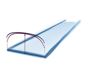
To quantify the effect of the mollification on the lift and drag distributions, a mollified lifting line (MLL) theory can be used (Caprace et al. 2019). The MLL is similar to the PLL, but the computation of the downwash is modified to account for the regularization of the vorticity field by a Gaussian kernel, as depicted in figure 6. The theory was developed for 3-D, 2-D and one-dimensional (1-D) mollifications, yet only the 2-D mollification is considered here. This way, the MLL is in accordance with the ALM that uses a 2-D Gaussian kernel for the force distribution. In this case, the downwash on the centreline of the mollified lifting line $\varepsilon _{\sigma,0}$ is obtained at each spanwise location by (Caprace et al. 2019)

(2.11)\begin{equation} \varepsilon_{\sigma,0}(y) =\frac{1}{U_{\infty}} \frac{1}{4 {\rm \pi}} \int_{{-}b / 2}^{b / 2}\left(\int_{-\infty}^{\infty} \frac{1}{\sqrt{\rm \pi}} \frac{{\rm e}^{{-}z^{\prime} / \sigma^2}}{((y-y^{\prime})^2+z^{\prime 2})} \frac{{\rm d} z^{\prime}}{\sigma}\right)(y-y^{\prime}) \frac{\mathrm{d} \varGamma}{\mathrm{d} y^{\prime}}(y^{\prime}) \,\mathrm{d} y^{\prime}. \end{equation}

The ALM used in this paper evaluates the effective velocity as a weighted average, using the weights of the distribution kernel, and not directly as that on the centreline. This approach, also known as integral sampling (Churchfield et al. 2017), is also included in the present MLL by adding a convolution of the induced velocity with the regularization kernel (Caprace et al. 2019). The resulting mean downwash $\bar {\varepsilon }_\sigma (y)$ is then given by

(2.12)\begin{align} \bar{\varepsilon}_\sigma(y) = \frac{1}{U_\infty} \frac{1}{4 {\rm \pi}} \int_{{-}b / 2}^{b / 2}\left[\iint_{-\infty}^{\infty} \frac{1}{\rm \pi} \frac{{\rm e}^{-{(z^{\prime 2}+z^{2})}/{\sigma^{2}}}}{((y-y^{\prime})^{2}+ (z-z^{\prime})^{2})} \frac{{\rm d} z^{\prime}}{\sigma} \frac{{\rm d} z}{\sigma}\right](y-y^{\prime}) \frac{{\rm d} \varGamma}{{{\rm d} y}^{\prime}}(y^{\prime})\, {{\rm d} y}^{\prime} . \end{align}

The lift distribution on the MLL is obtained similarly as for the PLL using (2.12) evaluated numerically. The downwash obtained using the mollified vortex sheet is, in general, smaller than that obtained using the singular vortex sheet of the PLL. This results in an overestimation of the lift force distribution on the wing, due to a higher effective angle of attack.

Figure 6. Mollified lifting line (MLL) with 2-D isotropic mollification (Caprace et al. 2019).

2.5. Vortex lattice method (VLM)

The vortex lattice method (also called lifting surface method) models the potential flow past a wing without thickness by dividing its surface into quadrilateral vortex rings, each consisting of four vortex segments in a closed-loop arrangement, as depicted in figure 7. The wake is represented by horizontal horseshoe vortices that extend to infinity. Each vortex ring has a circulation $\varGamma _{i,j}$, which is obtained by computing the downwash induced by all the elements and imposing no-through flow at the colocation point (located at the centre of each element). A detailed explanation is found from Katz & Plotkin (2001). The force $\boldsymbol {F}_{i,j}$ acting on each vortex segment is then obtained using the circulation $\varGamma _{i,j}$ of the segment, the velocity $\boldsymbol {U}_{i,j}$ measured at the centre of the segment and the segment vector $\boldsymbol {s}_{i,j}$ of norm equal to the segment length,

(2.13)\begin{equation} \boldsymbol{F}_{i,j} = \rho \boldsymbol{U}_{i,j} \times (\varGamma_{i,j} \boldsymbol{s}_{i,j}) . \end{equation}

For each wing section $j$, the lift per unit span is obtained as the sum of the vertical forces along the chord, divided by the length of each contributing segment,

(2.14)\begin{equation} l_j = \sum_{i=0}^{i=n_x} (\boldsymbol{F}_{i,j} \boldsymbol{\cdot} \hat{\boldsymbol{e}}_z)/\lVert\boldsymbol{s}_{i,j}\rVert . \end{equation}

The induced drag per unit span is obtained similarly from the force in the streamwise direction,

(2.15)\begin{equation} d_j = \sum_{i=0}^{i=n_x} (\boldsymbol{F}_{i,j} \boldsymbol{\cdot} \hat{\boldsymbol{e}}_x)/\lVert\boldsymbol{s}_{i,j}\rVert. \end{equation}

The total drag per unit span is then found by adding the profile drag obtained using the polar data and an estimated effective angle of attack. The latter is taken as the geometrical angle of attack minus the downwash angle induced by the trailing vortices, as measured at the wing quarter-chord line. The VLM is here used with $n_x=32$ in the chordwise direction and $n_y=128$ in the spanwise direction.

Figure 7. Vortex lattice method (VLM), here illustrated for a rectangular wing with $AR=7.5$ and $4 \times 30$ elements. The number of elements used in simulations is higher than depicted (32 in the chordwise direction, 128 in the spanwise direction).

3. Analysis of a rectangular wing with $AR=15$

In this section, the lift and drag distributions obtained using all the aforementioned methods for a rectangular wing of aspect ratio $AR = b/c=15$ are analysed. The geometry of the wing is represented in figure 8. The geometric angle of attack is set to 5$^\circ$, although the validity of the presented analysis extends to any small angle. The Reynolds number $Re_c$ is set to $6\times 10^6$. The mollification width is set to $\sigma = c/4$ for the ALM and the MLL, which corresponds to the optimal kernel width, according to Martínez-Tossas et al. (2017), as it minimizes the differences to the near field of airfoils in a 2-D flow.

Figure 8. Geometry of the rectangular wing of aspect ratio $AR=15$.

For the ALM simulation, the computational domain size is $12b\times 8b\times 8b$, which is sufficiently large to represent unbounded conditions. Here, 128 grid points are set per wing span: $b/h=128$. This leads to a sufficient discretization of the Gaussian kernel since $\sigma /h=128/60\simeq 2.13 \ge 2$ (Troldborg 2008). The time step is set to 0.002 second, which corresponds to a Courant–Friedrichs–Lewy number of 0.256. The ALM simulation is run for 3600 time steps, which is sufficient to reach steady state with a fully developed wake. The inflow velocity is uniform and contains no turbulence. The steady-state RANS simulations also consider a uniform inflow without turbulence. The wake of the wing is steady and contains no turbulence. The RVM sub-grid scale model is therefore not active (indeed, an RVM model is only active in regions with turbulence (Jeanmart & Winckelmans 2007)). The loads obtained using the ALM are thus also steady and can be compared with those obtained using the wall-resolved simulations.

The lift and drag distributions along the wing half-span are displayed in figure 9. The integrated lift and drag coefficients are also reported in Appendix E. The lift distributions are considered first and differ substantially near the tip depending on the method. First, one observes that the present MLL and ALM agree very well. Indeed, the forces of the ALM are distributed using the same 2-D Gaussian kernel as that used for the mollification of the vorticity field considered in the MLL. Both also use the same integral velocity sampling. A mollified vortex sheet is produced behind the ALM by the flow solver, and it is here sufficiently resolved to induce a velocity on the actuator line that matches the induction predicted by the MLL. The resulting lift and drag distributions are therefore virtually identical. However, both the ALM and MLL predict a higher lift distribution than the PLL. This deviation is attributed to the mollification of the shed vortex sheet that reduces the velocity induced by the wake. As a result, the integrated lift coefficient of the wing, $C_L$, increases from 0.476 for the PLL to 0.486 ($+2.6\,\%$) for the ALM/MLL. However, the PLL also predicts higher lift forces in the near-tip region compared with the VLM and the reference. These differences are due to the variation of the induced velocity along the chord that are not correctly captured when the wing surface is not represented. This effect is known at the ‘virtual camber effect’ (Sørensen et al. 2016) and modifies the aerodynamic properties of the profile, as described in § 1. In the ALM, MLL and PLL, the velocity is only sampled at the quarter chord position, and hence does not account for the uneven downwash along the chord, resulting in an over-prediction of the loads. As a result, the $C_L$ of the PLL is 1.5 % higher than that of the VLM and of the reference results ($C_L=0.467$). Finally, one observes that the VLM predicts a similar lift distribution as that of the reference wall-resolved simulation. In fact, the VLM models the wake using singular trailing vortices and accounts for the virtual camber, as it evaluates the downwash on the entire wing surface. The good agreement between the reference simulation results and the VLM implies that the mollification and virtual camber are the main factors influencing the lift distribution of the ALM compared with the reference results. Conversely, the effect of the formation of the tip vortex on the upper wing surface only affects the flow on a very small distance to the tip, which is not modelled by the present ALM (Chow et al. 1997). The effect of the spanwise velocity also does not affect the loads. In fact, the spanwise velocity components on the upper and lower surfaces near the tip are of opposite sign and of similar amplitude, and they tend to compensate each other as far as the lift and drag coefficients are concerned.

Figure 9. Comparison of the lift and drag coefficient distributions computed using various methods along the wing half-span of a rectangular wing with $AR=15$ at angle of attack $\alpha =5^\circ$. The wall-resolved RANS simulation (Reference wrRANS) is used as reference. The integrated $C_L$ and $C_D$ coefficients are provided in Appendix E.

The drag distribution is largely overpredicted in the near-tip region by both the PLL and the MLL/ALM. However, it is interesting to observe that the MLL and ALM predict lower values than the PLL. This arises from the fact that the drag ((2.4)) contains two components: the profile drag, which accounts for friction and form drag, and the induced drag, which arises from the tilt of the lift vector. These two components are obtained separately in the MLL and PLL, and are depicted in figure 10. The mollification increases the effective angle of attack $\alpha _e$, which also slightly increases the profile drag of the MLL near the tip. However, the value of the induced drag of the MLL is decreased to a larger extent due to the reduced downwash angle. This leads to an overall reduction of the drag distribution in the near-tip region, although it still remains different from the reference results. The drag distribution obtained by the VLM is also slightly different from that of the wall-resolved simulations. In fact, the VLM does not account for the profile thickness and for the viscous effects. Whereas these effects are of minimal importance on the lift distribution, their influence over the drag is more pronounced, leading to some deviation in the outer part of the wings.

Figure 10. Comparison of the profile and induced drag coefficient distributions ($C_{d,p}$ and $C_{d,i}$, respectively) in the wing outer region.

4. Near-tip correction functions for the lift and drag distributions

4.1. Correction function for the lift coefficient

The previous section has shown that the ALM overpredicts the lift and drag distributions compared with the reference results, due to the mollification and the virtual camber effects. In this section, a correction function $F_l$ for the lift is obtained to account for these effects. Since this function aims at correcting the near-tip behaviour, it is expressed as a function of the distance to the tip $d_{tip}(y)$, normalized by the chord $c$. The distance to the tip is defined as (see figure 8)

(4.1)\begin{equation} d_{tip}(y) = \frac{b}{2} - |y|,\end{equation}

which is valid for both sides of the wing. The correction function for the lift is defined as the difference between the non-corrected lift coefficient distribution predicted by the ALM, denoted $C_l^{ALM,nc}(y)$, and the lift coefficient distribution of the reference, denoted $C_l^{ref}(y)$. For the sake of conciseness, the dependency to $y$ is not written explicitly in the equations that follow. The function $F_l$ reads

(4.2)\begin{equation} F_l\left(\frac{d_{tip}}{c}\right) = \frac{(C_l^{ALM,nc}-C_l^{ref})}{C_l^{ALM,nc}}.\end{equation}

It can then be applied to obtain the corrected lift coefficient $C_{l}^{corr}(y)$ as

(4.3)\begin{equation} C_{l}^{corr} = \left( 1-F_l\left(\frac{d_{tip}}{c} \right) \right) C_{l}. \end{equation}

The application of the correction is here illustrated for the rectangular wing with ${AR=15}$. It is first necessary to converge the correction function $F_l$ using multiple iterations, as the modification of the lift coefficient also modifies the wake and hence the induced velocity. The obtained correction function is depicted in figure 11, and its numerical values are also provided in Appendix C. In this case, three iterations were sufficient to reach convergence. The resulting correction function is maximal near the wing tip, and it decreases with the distance to the tip. The value of the correction is below 1 % for $d_{tip}/c \ge 3.5$. Hence, a correction must be applied on a significant region in the outer part of the wing.

Figure 11. Correction function $F_l$ for the lift coefficient. The final function (in dark blue) is obtained in three iterations.

To verify that the current analysis is valid for any small angle of attack, for which the profile lift coefficient increases linearly, the correction function for the lift is obtained for various small angles. The result of this investigation is shown in figure 12. It is shown that the correction function is essentially the same regardless of the angle of attack. This results from the fact that the effect of the mollification and the virtual camber effect both increase linearly with the angle of attack.

Figure 12. Correction functions $F_l$ obtained for various angles of attack.

The results obtained with the ALM and the MLL after the application of the correction function are displayed in figure 13, and compared with the reference results. As expected, the corrected lift is now virtually identical to that of the reference. However, the distribution of the drag changed importantly, and it now decreases near the tip. This is due to the reduction of the downwash caused by the lift correction and that reduces the induced drag component. It is therefore necessary to also apply a correction function for the drag distribution.

Figure 13. Lift and drag distributions before and after application of the correction function $F_l$ for the lift, for the case of a rectangular wing with $AR=15$ at $\alpha =5^\circ$.

4.2. Correction function for the angle of attack

To correct the drag distribution, it is tempting to define a similar function $F_d$ that would act on the drag coefficient,

(4.4)\begin{equation} F_d\left(\frac{d_{tip}}{c}\right) = \frac{(C_d^{ALM,nc}-C_d^{ref})}{C_d^{ALM,nc}}. \end{equation}

However, the previous analysis (reported in figure 10) has shown that the error on the drag coefficient is mostly related to the induced drag, whose value, given by (2.4), depends on the downwash angle. In fact, provided that the profile drag remains essentially constant in the considered region of the wing, and that the lift coefficient is corrected to match the reference results, then the error on the drag distribution necessarily originates from a misprediction of the downwash. As also shown by Pirrung et al. (2020), it is therefore preferable to correct the effective angle of attack to obtain the correct drag, while also maintaining a correct value for the lift. This is possible due to the small value of the downwash angle. Following (2.3), the lift of the wing is very close to the lift of the profile $C_l \simeq C_l^p$. Moreover, for small angles of attack, the profile lift coefficient is a linear function: $C_l^p(\alpha ) \simeq ({{\rm d} C_l^p}/{{\rm d} \alpha }) \alpha$. The corrected lift coefficient, given by (4.3), can thus be rewritten as

(4.5)\begin{equation} C_l^{corr} \simeq \left( 1-F_l\left(\frac{d_{tip}}{c} \right) \right) \frac{{\rm d} C_l^p}{{\rm d} \alpha} \alpha_e. \end{equation}

Then the correction function $(1-F_l)$ can then be split into two parts: one that applies to the derivative of the profile lift coefficient, denoted $(1-F_{C_l})$, and the other that applies to the effective angle of attack, denoted $(1-F_{\alpha _e})$. This leads to the following expression:

(4.6)\begin{equation} C_l^{corr} = \left( 1-F_{C_l}\left(\frac{d_{tip}}{c} \right)\right) \frac{{\rm d} C_l^p}{{\rm d} \alpha} \left( 1-F_{\alpha_e}\left(\frac{d_{tip}}{c} \right) \right) \alpha_e . \end{equation}

To ensure that the correction of the lift remains unchanged, the condition that $(1-F_l) = (1-F_{C_l})(1-F_{\alpha _e})$ must be enforced. To complete the correction, it is then only necessary to find the function $F_{\alpha _e}$ that modifies the effective angle of attack.

The value of the downwash is not directly measured from the wall-resolved simulations, but can be obtained using the lift and drag distribution and the profile drag coefficient. In fact, (2.4) allows for expressing the reference downwash $\varepsilon ^{ref}(y)$ as

(4.7)\begin{equation} \varepsilon^{ref} = \frac{(C_d^{ref} - C_d^{p}(\alpha-\varepsilon^{ref}))}{ C_l^{ref} }. \end{equation}

This equation can be solved iteratively. Then, the correction function for the effective angle of attack is defined in a similar manner as for the correction function for the lift (4.2) by

(4.8)\begin{equation} F_{\alpha_e}\left(\frac{d_{tip}}{c}\right) = \frac{((\alpha-\varepsilon^{ALM,nc})-(\alpha- \varepsilon^{ref}))}{(\alpha -\varepsilon^{ALM,nc})} = \frac{(\alpha_e^{ALM,nc}-\alpha_e^{ref})}{\alpha_e^{ALM,nc}}. \end{equation}

Note that for an airfoil without camber, the profile drag coefficient is well approximated by a quadratic function $C_d^p(\alpha ) \simeq C_{d,0}^p + \beta \alpha ^2$ (see Appendix A). In this case, (4.7) can also be solved analytically.

The corrected value of the effective angle of attack $\alpha _e^{corr}(y)$, used to evaluate the lift and drag coefficients, is therefore given by

(4.9)\begin{equation} \alpha_e^{corr} = \left( 1-F_{\alpha_e}\left(\frac{d_{tip}}{c} \right) \right)\alpha_e. \end{equation}

The corrected value of the downwash angle $\varepsilon ^{corr}(y)$, used for the evaluation of the induced drag, is found as

(4.10)\begin{equation} \varepsilon^{corr} = \alpha - \alpha_e^{corr}. \end{equation}

Finally, the corrected value of the drag coefficient $C_d^{corr}$ is obtained from (2.4) as the sum of the corrected profile drag coefficient and of the corrected induced drag,

(4.11)\begin{equation} C_d^{corr} = C_d^{p}(\alpha_e^{corr}) + C_l^{corr} \varepsilon^{corr}. \end{equation}

The decomposition of $F_l$ into $F_{C_l}$ and $F_{\alpha _e}$ for the rectangular wing with $AR=15$ is depicted in figure 14. The numerical values of these functions are also provided in Appendix C. It can be seen that the correction of the angle of attack is mostly necessary close to the tip, until a distance $d_{tip}/c \simeq 1$. This indeed corresponds to the region where the drag of the ALM corrected for the lift coefficient differs from the reference results. Further away from the tip, the correction mostly acts on the profile lift coefficient. The value of that correction only drops below 1 % for $d_{tip}/c \ge 3.5$.

Figure 14. Decomposition of $F_l$ into $F_{\alpha _e}$ and $F_{C_l}$ such that $(1-F_l)=(1-F_{C_l})(1-F_{\alpha _e})$.

The results of the simulations performed by applying the correction functions is displayed in figure 15. Clearly, the correction significantly improves the accuracy of the drag distribution, which is now consistent with the reference results. The lift distribution also remains in good agreement with the reference. We also note that solely correcting the ALM for the mollification effect to reproduce the PLL results would not be sufficient in the present case.

Figure 15. Lift and drag coefficient distributions before and after application of the correction functions for the lift coefficient $F_{C_l}$ and for the effective angle of attack $F_{\alpha _e}$ on the rectangular wing with $AR=15$ at $\alpha =5^\circ$.

Note that applying the correction causes an increase of the lift computed on the last control point of the ALM. This originates from the small spanwise mollification of the ALM caused by the distribution of the forces from the template plane to the closest flow grid points. This slightly reduces the induced velocity near the tip. The MLL is purely based on a mathematical formula without any spanwise mollification, and therefore it does not predict an increase of the lift at the tip. When the correction is applied to the ALM, the effect of the small spanwise mollification becomes more significant, leading to a difference with the MLL at the last control point. However, the MLL and the ALM show a very good agreement at the other control points.

The correction functions were here obtained for a rectangular wing with a high aspect ratio ($AR=15$). However, their application to rectangular wings with lower aspect ratios must also be considered. In the next section, it is verified that the obtained correction functions remain valid for wings down to $AR=7.5$.

5. Investigation of rectangular wings down to $AR=7.5$

The validity of the correction functions is also assessed on two rectangular wings with smaller aspect ratios: $AR=10$ and $AR=7.5$. For the MLL and the ALM, the mollification parameter $\sigma$ is kept at $\sigma = c/4$. The computational set-up used for the simulations with the ALM is unchanged. We use $b/h=96$ for $AR=10$ (hence, $\sigma /h=2.4$) and $b/h=64$ for $AR=7.5$ (hence, $\sigma /h\simeq 2.13$).

For both aspect ratios, the correction functions $F_l$, $F_{C_l}$ and $F_{\alpha _e}$ are obtained by comparing the results of wall-resolved RANS simulations with those of the ALM/MLL, following the methodology of § 4, and are depicted in figure 16. We confirm that the obtained functions are very similar for all investigated aspect ratios. Consequently, the correction functions established for $AR=15$ in the previous section can also be used for cases with lower aspect ratio, at least down to $AR=7.5$, without modification.

Figure 16. Correction functions (a) $F_l$, (b) $F_{C_l}$ and (c) $F_{\alpha _e}$ measured exactly for the three aspect ratios.

The lift and drag distributions predicted by the corrected ALM/MLL, and using the correction functions established for $AR=15$, are shown in figure 17 and are compared with those of the uncorrected methods and of the reference. We see that decreasing the wing aspect ratio significantly decreases the accuracy of the uncorrected ALM and that the discrepancies with the reference results span a larger part of the wing. Again, those errors are not solely related to the mollification, since the PLL also fails to recover the correct load distribution. Applying the correction leads to a much better agreement with the reference results, on both the lift and drag distributions, for each aspect ratio. Note that, for the case $AR=7.5$, the corrections affect almost the entire wing since the maximal value of $d_{tip}/c$ is 3.75.

Figure 17. Lift and drag coefficient distributions before and after application of the correction functions $F_{C_l}$ and $F_{\alpha _e}$, and for the rectangular wings at $\alpha =5^\circ$. (a) $AR = 10$ and (b) $AR = 7.5$.

It can therefore be concluded that the proposed correction functions, which are solely expressed in terms of $d_{tip}/c$, perform quite well for rectangular wing down to $AR=7.5$. In the next section, we assess the performance of the correction functions for linearly tapered wings.

6. Investigation of linearly tapered wings

In this section, wings with linear taper are considered, which means that the chord varies linearly along the wing span, as illustrated in figure 18. The taper ratio $\varLambda$ is defined as the ratio of the chord at the tip to that at the wing centre, $\varLambda = c_{tip}/c_{root}$. The aspect ratio is defined using the mean chord $\bar {c}=S/b$, and hence $AR=b/\bar {c}=b^2/S$.

Figure 18. Geometry of a linearly tapered wing with $AR=10$ and $\varLambda =1/3$.

Considering the right part of the wing, the chord variation is given by

(6.1)\begin{equation} c(y) = c_{root} + \frac{{\rm d}c}{{\rm d} y} y, \end{equation}

where ${\rm d}c/{{\rm d} y}<0$. We also have that

(6.2)\begin{equation} \left| \frac{{\rm d}c}{{\rm d} y} \right| = \frac{4}{AR} \frac{(1-\varLambda)}{(1+\varLambda)} . \end{equation}

Four tapered wings are considered, with aspect ratios $AR=15$ and $10$, and taper ratios $\varLambda =1/2$ and $1/3$, as summarized in table 1. The cases are sorted by the absolute value of the chord variation. Note that case 2 and case 3 have the same value of $|{\rm d}c/{{\rm d} y}|$.

Table 1. Studied tapered wings.

For the ALM and the MLL, the mollification parameter is again kept constant along the span and is scaled based on the mean chord: $\sigma =\bar {c}/4$. The computational domain of the ALM simulations are the same as for the rectangular wing cases, and the resolution depends on the aspect ratio: $b/h=128$ ($\sigma /h\simeq 2.13$) for $AR=15$ and $b/h=96$ (${\sigma /h=2.4}$) for $AR=10$.

The dimensionless distance to the wing tip must also be redefined as the chord varies. We will use an effective dimensionless distance to the tip defined using a cumulative integral. For the right part of the wing, it is defined as

(6.3)\begin{equation} \left( \frac{d_{tip}}{c} \right)_{eff}(y) = \int_{y}^{b/2} \frac{{{\rm d} y}'}{c(y')}. \end{equation}

For the left part of the wing, it reads

(6.4)\begin{equation} \left( \frac{d_{tip}}{c} \right)_{eff}(y) = \int_{{-}b/2}^{y} \frac{{{\rm d} y}'}{c(y')}. \end{equation}

The value of the integral is the same on both parts,

(6.5)\begin{equation} \left( \frac{d_{tip}}{c} \right)_{eff}(y) = \frac{1}{|{\rm d}c/{{\rm d} y}|} \log\left(1+\left| \frac{{\rm d}c}{{\rm d} y} \right|\frac{\left(b/2-|y|\right)}{c_{tip}}\right). \end{equation}

Note that for the case of a rectangular wing, we recover

(6.6)\begin{equation} \left( \frac{d_{tip}}{c} \right)_{eff}(y) =\frac{d_{tip}(y)}{c} = \frac{1}{c} \left(\frac{b}{2} - |y|\right). \end{equation}

The lift and drag distributions predicted by all methods are first analysed on the various tapered wings. Those are depicted in figure 19. For clarity, only the near-tip region of the wing is shown, which corresponds to $0.3 \le y/b \le 0.5$. One should however note that the ‘line’ methods also differ from the reference at the centre of the wing due to the virtual camber effect. This difference is discussed in Appendix D, and we here focus on the error in the near-tip region. The lift distribution obtained using the VLM is again in very good agreement with that of the reference. The PLL overpredicts the lift near the tip, yet its accuracy is better for the smaller taper ratio (i.e. $\varLambda =1/3$). This indicates that the influence of the virtual camber effect is reduced when the chord diminishes near the tip. Indeed, the effect of the variation of the induced velocity along the chord is less pronounced when the chord is smaller (Sørensen et al. 2016). Moreover, the magnitude of the shed vortex sheet, and hence of the induced velocity, is also smaller near the tip of a tapered wing due to a smoother decrease of the lift along the span. Again, the uncorrected ALM and MLL overpredict the lift compared with the PLL.

Figure 19. Lift and drag coefficient distributions for tapered wings with various aspect and taper ratios for $\alpha =5^\circ$. (a) Case 1 ($AR=15$ and $\varLambda =1/2$), (b) case 2 ($AR=15$ and $\varLambda =1/3$), (c) case 3 ($AR=10$ and $\varLambda =1/2$) and (d) case 4 ($AR=10$ and $\varLambda =1/3$).

The drag distribution of the various wings is also depicted in figure 19. The drag predicted by the ALM and MLL is lower than that predicted by the PLL due to the smaller value of the induced drag. It is therefore in better agreement with the reference; however, this cannot be considered correct as it follows from a spurious reduction of the downwash.

The exact correction functions, obtained using the methodology described in § 4, are displayed in figure 20 for each case. The functions for the case of a rectangular wing with $AR=15$ is also displayed as a reference. The correction function for the lift only, $F_l$, is similar for all tapered cases and is indeed essentially that of the rectangular wing. This indicates that the correction for the lift is also valid for tapered wings when expressed in terms of the effective dimensionless distance to the tip, $(d_{tip}/c)_{eff}$. This result is most important as it shows that using the proposed effective scaling allows for obtaining a unique correction function for the lift; something that most correction methods aim to do.

Figure 20. Correction functions (a) $F_l$, (b) $F_{C_l}$ and (c) $F_{\alpha _e}$ measured exactly for the tapered wings. The functions measured for the rectangular wing with $AR=15$ are also displayed.

The correction of the drag distribution, obtained through a correction of the effective angle of attack, is also tested for tapered wings. The decomposition of $F_l$ into its two components $F_{C_l}$ and $F_{\alpha _e}$ differs slightly depending on the taper ratio, even though the general behaviour of the functions remains the same. A smaller taper ratio leads to a larger $F_{\alpha _e}$, and hence a smaller $F_{C_l}$.

The application of the correction functions is tested on the different cases. The results are first depicted in figure 21 for the lift distribution. For the sake of clarity, only the results obtained using the MLL are shown (those were verified to be in very good agreement with those of the ALM). Two sets of correction functions are considered: the exact functions as shown in figure 20 and the functions obtained for the rectangular wing. The results show that the lift distribution is the same for both corrections and is in a very good agreement with that of the reference. The correction function for the lift coefficient is hence verified to be valid regardless of the taper ratio, as long as the effective normalized distance to the tip, $(d_{tip}/c)_{eff}$, is correctly defined.

Figure 21. Lift distribution for different tapered wings before and after correction. (a) Case 1 $(AR =15, \varLambda =1/2)$; (b) case 2 $(AR =15, \varLambda =1/3)$; (c) case 3 $(AR =10, \varLambda =1/2)$ and (d) case 4 $(AR =10, \varLambda =1/3)$.

The drag distribution is displayed for the various cases in figure 22. Again, the MLL is tested with the exact correction functions and with those of the rectangular wing. When using the exact correction, the drag distribution is in very good agreement with the reference results. If the correction obtained for the rectangular wing is used instead, the drag at the tip tends to be slightly underpredicted. This discrepancy is also more pronounced for the smaller aspect ratio $\varLambda =1/3$. However, applying the functions $F_{C_l}$ and $F_{\alpha _e}$ of the rectangular wing is still better than only applying the correction function $F_l$ for the lift: the behaviour of the drag remains consistent with the reference when using $F_{C_l}$ and $F_{\alpha _e}$, whereas it quickly decreases near the tip when using solely $F_l$. Moreover, for $\varLambda =1/2$, the accuracy of the drag predicted using the corrected MLL is better than that of the PLL. For $\varLambda =1/3$, the agreement is similar.

Figure 22. Drag distribution for different tapered wings before and after correction. (a) Case 1 $({AR =15}, {\varLambda =1/2})$; (b) case 2 $(AR =15, \varLambda =1/3)$; (c) case 3 $(AR =10, \varLambda =1/2)$ and (d) case 4 $({AR =10}, {\varLambda =1/3})$.

7. Effect of the mollification size and type

7.1. Effect of the mollification size

The mollification size, parametrized by the ratio $\sigma /c$, affects the accuracy of the loads predicted by the ALM importantly. In the previous sections, the size of the mollification was fixed to $\sigma /c=1/4$, as suggested by Martínez-Tossas et al. (2017). However, the mollification must sometimes be enlarged for practical applications. In this section, the effect of a change of the mollification size over the correction functions is considered. Simulations of the rectangular wing with $AR=15$ are performed using various values of $\sigma /c$. The results of these simulations are shown in figure 23. The MLL still provides excellent predictions for the ALM results with the larger mollifications. The lift coefficient further differs from the wall-resolved simulation and PLL results as the size of $\sigma /c$ increases, and the effect of the mollification becomes more significant than that of the virtual camber. The drag coefficient is also affected by the value of $\sigma /c$. This illustrates that the effect of the mollification impacts both the lift and the drag by changing the induced velocity on the wing.

Figure 23. Comparison of the lift and drag coefficients distributions along the half-span of the rectangular wing with $AR=15$ at $\alpha =5^\circ$, computed using various methods. The black markers are the results of the wall-resolved simulations.

The evolution of the integrated $C_L$ and $C_D$ with the mollification size is shown in figure 24. These are obtained using the MLL with various mollifications, up to $\sigma /c=2$. The integrated lift coefficient substantially increases with the mollification size: it is 2 % higher than the reference without mollification (PLL), whereas it reaches 8 % for the largest $\sigma /c$. The integrated drag coefficient decreases with the mollification size, starting from an overestimation of 6.3 % (PLL) to an underestimation of $-5\,\%$.

Figure 24. Evolution of the $C_L$ and $C_D$ with the mollification size for a rectangular wing with $AR=15$: effect of the 2-D mollification (black dots) and of the 3-D mollification (blue squares).

The correction functions obtained by comparing the MLL with the various mollification sizes to the reference results are provided in figure 25, and tables with the numerical values are provided in Appendix C. The functions $F_{C_l}$ for the lift coefficient are very similar for the various mollification sizes. This indicates that this function mostly corrects the effect of the virtual camber. The virtual camber indeed mostly depends on the lift variation along the wing span and of the chord, which remains essentially constant regardless of the mollification size.

Figure 25. Correction functions for (a) the lift coefficient $F_{C_l}$ and for (b) the angle of attack $F_{\alpha _e}$ for various mollification sizes in the case of a rectangular wing with $AR=15$.

The function $F_{\alpha _e}$ for the effective angle of attack evolves importantly with the increase of the mollification size, which indicates that the effect of the mollification can be corrected for both the lift and the drag by adapting the induced angle of attack. This is consistent with the fact that the mollification of the shed vortex sheet alters the value of the induced velocity on the wing, and hence mostly affects the effective angle of attack and not the lift coefficient. The function also extends to a larger distance to the tip $(d_{tip}/c)$ when the mollification size increases. However, in all cases, the product of the correction functions remains lower than 1 % for $(d_{tip}/c) \gtrsim 3.5$.

7.2. Effect of the mollification type

Whereas the 2-D mollification has been shown to lead to a better evaluation of the loads compared with a 3-D mollification by Caprace et al. (2019), the 3-D mollification is still used by many authors (Martínez-Tossas & Meneveau 2019; Meyer Forsting et al. 2019; Dag & Sørensen 2020; Kleine et al. 2023a). One justification for the use of a 3-D mollification is that the spanwise mollification decreases the force gradient at the tip and produces a smoother tip vortex. In some numerical methods, sharp gradients could potentially be problematic for numerical stability. Therefore, the case of a 3-D mollification is here also evaluated and corrected on the rectangular wing with $AR=15$. The variation of the loads near the tip and the correction functions are compared with those obtained using a 2-D mollification.

For the ALM, the use of a 3-D mollification consists in distributing the forces of each control point using a 3-D Gaussian kernel. For consistency, integral sampling is also used: the velocity at each control point is obtained as a weighted averaged using the same 3-D kernel. The MLL with 3-D mollification is obtained by replacing the expression of the downwash in (2.12) by (see Caprace et al. 2019)

(7.1)\begin{equation} \bar{\varepsilon}_\sigma(y)=\frac{1}{U_{\infty}} \frac{1}{4 {\rm \pi}} \int_{{-}b / 2}^{b / 2} \frac{(1-{\rm e}^{-((y-y^{\prime})^2 / 2 \sigma^2)})}{(y-y^{\prime})} \frac{\mathrm{d} \varGamma}{\mathrm{d} y^{\prime}}(y^{\prime}) \,\mathrm{d} y^{\prime}. \end{equation}

The integral is also evaluated numerically.

Figure 26 shows the lift and drag distributions computed using the ALM and the MLL with 3-D mollification. The agreement between the MLL and the ALM is again very good. The comparison between the 2-D and 3-D mollifications indicates a clear deviation in lift and drag near the tip. The spanwise mollification reduces the induced velocity at the tip, and the downwash measured on the last control points of the ALM is therefore smaller. As a result, the lift is higher due to the larger effective angle of attack, whereas the drag decreases due to the effect of the downwash on the induced drag. The region of the wing affected by the 3-D mollification grows with the size of the mollification parameter $\sigma /c$. This region is of size $\simeq 2 \sigma$, and the number of control points affected by the spanwise mollification near the tip is thus related to the ratio $\sigma /h$. Interestingly, for the case $\sigma =c/4$, some deviations between the 2-D and 3-D mollifications are also visible in the range $0.425< y/b<0.475$. These arise from the fact that this region presents a larger gradient of the forces along the span, whose value is affected by the spanwise mollification. Figure 24 also presents the integrated $C_L$ and $C_D$ coefficients depending on the 3-D mollification size. They differ more from the reference than those obtained using the 2-D mollification, and this difference further increases with the mollification size.

Figure 26. Lift and drag coefficients on the rectangular wing with $AR=15$ at $\alpha =5^\circ$, obtained using ALM/MLL with 2-D or 3-D mollification, compared with the PLL and the reference wrRANS.

The correction functions are also obtained for the case of 3-D mollification, and are depicted in figure 27. Although the lift and drag distributions are not monotonic near the tip, the correction functions have an aspect similar to those obtained for the 2-D mollification. Specifically, the functions for the lift coefficient $F_{C_l}$ are very similar, regardless of the mollification type and size. Only the last two control points present a small deviation. In contrast, the functions for the effective angle of attack $F_{\alpha _e}$ present significantly higher values at a small normalized distance to the tip. Again, this indicates that the effect of the mollification can be mitigated by changing only the effective angle of attack and the downwash angle.

Figure 27. Correction functions obtained for the rectangular wing with 3-D mollification of different sizes and also compared with those obtained with 2-D mollification.

8. Application to NREL phase VI wind turbine and comparison to experimental data

In this section, the correction functions are applied to the case of a horizontal axis wind turbine and compared with the experimental data from the NREL Phase VI Unsteady Aerodynamic Experiment (Hand et al. 2001). The NREL Phase VI rotor consists of two linearly tapered blades with an aspect ratio $AR\simeq 7$ and a taper ratio $\varLambda \simeq 1/2$, as depicted in figure 28. It has a total diameter $D$ of 10.058 m. The blades consist of a single airfoil profile, the NREL S809, and are slightly twisted near the tip. The polar data used for the ALM are those provided by Jonkman (2003). The Sequence S tests are here considered, which corresponds to the case of an upwind rotor with a tip pitch of 3$^\circ$ (corresponding to a pitch angle of 4.815$^\circ$ relative to the zero pitch axis). The tests performed with a uniform wind speed of 6 m s$^{-1}$ and a constant rotation speed of 71.9 rpm are considered to keep the angle of the attack in the near-tip region to a moderate value.

Figure 28. Geometry of the NREL Phase VI blade, with the pressure taps located at $y/b=0.3$, 0.466, 0.633, 0.8 and 0.95.

Although the correction functions were derived for a wing without twist, they can be applied to the case of a wind turbine blade, since the light twist $\gamma (r)$ essentially compensates the variation of the local rotation velocity $\varOmega r$ along the span, so that the geometrical angle of attack, $\arctan ({U_\infty /(\varOmega r)})-\gamma (r)$, is mostly constant on the last three chords of the blades. The functions are therefore applied as described in § 4.2 and accounting for the change of the geometrical angle of attack along the span: $\alpha =\alpha (y)$.

For the ALM simulations, the computational domain size is 8$D$ in the streamwise direction and 3$D$ in the lateral directions, which results in the same blockage factor as that of the experimental wind tunnel (defined as the ratio between the rotor swept area and the wind tunnel cross-section, here $\simeq 10\,\%$). The mesh is Cartesian and consists of $1024 \times 512 \times 512$ grid points, resulting in a resolution of $\simeq 170$ grid points per rotor diameter. The time increment is chosen to obtain 600 time steps per rotation, ensuring that the blade tip does not go through more than one grid-cell per time step. The effect of the 2-D mollification size is also assessed by comparing three parameters : $\sigma /\bar {c}=1/4$, 1/2 or 1, where $\bar {c}=0.54$ m.

The loads distributions are depicted in figure 29 from $r/R=0.25$, which corresponds to the region of the blade with an aerodynamic profile. They are compared with those obtained experimentally or using the blade element momentum theory (BEM). The BEM uses the same polar data as the ALM and uses Prandtl's tip-loss factor to account for the effect of the individual blades (Glauert 1935). For the corrected ALM simulations, the functions accounting for the mollification size are used, see figure 25.

Figure 29. Normal and tangential coefficients (relative to the local airfoil chord line) along the blade span of the NREL Phase VI rotor operating under an inflow of 6 m s$^{-1}$ with a tip pitch of 3$^\circ$ (NREL Phase VI S06 series).

The uncorrected ALM is in a good agreement with the experimental data up to $r/R \simeq 0.8$. Beyond that, it fails to predict the decrease of the forces. As discussed previously, the use of larger mollification sizes further overpredicts the loads in that region. The application of the correction functions reduces the loads in the near-tip region importantly, resulting in a much improved agreement with the experimental data. It also removes the effect of the mollification size efficiently, as the obtained load distributions are similar for the three mollifications.

Additionally, the loads obtained in the near-tip region are more consistent with the experimental data than those predicted using the BEM. This originates from the ability of the correction functions to also account for the effect of the virtual camber, which is not considered in the BEM. For $r/R \le 0.9$, the BEM results are noticeably below those of the ALM. This variation is a consequence of the smaller induced velocity that results in a higher effective angle of attack and higher loads. It can be partly attributed to the fact that the BEM does not account for any blockage effect.

The effect of the correction on the rotor thrust and power coefficient is considerable, as reported in table 2. Using the uncorrected ALM leads to higher prediction of the rotor thrust and power compared with using the experimental data. Additionally, the effect of the mollification is clear on the thrust and on the power, which increase respectively by 4.4 % and 6.9 % as the mollification size increases from $\sigma =\bar {c}/4$ to $\sigma =\bar {c}$. Applying the correction functions reduces both the thrust and the power coefficient by approximately $5\,\%$ with the smallest mollification, and by 8 to 10 % for the largest one. The effect of the mollification is much decreased by the correction, as the thrust and power coefficient remain close as the parameter $\sigma /\bar {c}$ increases.

Table 2. Thrust and power coefficients of the NREL Phase VI rotor at 6 m s$^{-1}$ (NREL Phase VI S06 series). Percentages of difference are given relative to the experimental value.

9. Conclusions

The actuator line method (ALM) has become increasingly used in recent years, especially for wind energy related applications. However, the accuracy of the loads obtained with this method decreases significantly in the near-tip region. This study aims at investigating the sources of these inaccuracies by simulating translating wings using various methods. The lift and drag distributions predicted using high-fidelity wall-resolved simulations are compared with those obtained using the ALM, the Prandtl lifting line method, the mollified lifting line method and the vortex lattice method.

Rectangular wings with different aspect ratios ($AR=15$, 10 and 7.5) are first considered. For this geometry, the lift and drag distributions predicted by the ALM differ significantly from the reference results in the near-tip region (i.e. where the distance to the tip is smaller than approximately 3 chords). The differences are shown to not only arise from the mollification of the forces, but also from the variation of the induced velocity along the chord (known as the virtual camber effect). Indeed, the singular Prandtl lifting line method also fails to accurately predict the lift in this region and also overpredicts the drag coefficient. In contrast, the vortex lattice method, which naturally accounts for this effect, is in excellent agreement with the reference simulations for the lift and induced drag. Consequently, it can be argued that a near-tip correction that solely removes the influence of the mollification is not sufficient. Based on this investigation, correction functions for the lift coefficient and for the effective angle of attack are developed, so that the improved ALM is then able to reproduce both the lift and drag distributions of the reference results. These functions are expressed in terms of the distance to the wing tip normalized by the chord. Their application is shown to lead to a much better prediction of the lift and drag distributions for all investigated aspect ratios.

The case of tapered wings is then also studied, for two aspect ratios ($AR=15$ and 10) and two taper ratios ($\varLambda =1/2$ and 1/3). In these cases, the chord decreases linearly towards the tip. The correction functions obtained for the rectangular wing are also successfully applied to the tapered wings by defining an effective dimensionless distance to the tip, $(d_{tip}/c)_{eff}$, obtained using a cumulative integral. With this scaling, the correction function for the lift is seen to be applicable to all investigated taper ratios. For the drag, the correction function for the effective angle of attack is slightly affected by the taper ratio. However, the application of the correction functions for the rectangular wing still leads to an improved drag distribution.

The effects of the mollification size and type are then also investigated. The uncorrected ALM using the 2-D Gaussian mollification is confirmed to be more accurate in the near-tip region than when using the 3-D mollification. The correction functions are then obtained for different mollification sizes (different $\sigma /c$) and types (2-D and 3-D). The correction function for the lift coefficient is shown to be unaffected by the changes of the mollification parameters (both size and type), whereas the correction function for the effective angle of attack increases for larger mollification sizes and for the 3-D mollification. It is therefore concluded that the correction function for the lift coefficient is mostly related to the virtual camber effect, while the correction function for the effective angle of attack is related to the mollification. Finally, the case of the NREL Phase VI experimental rotor is considered, and the application of the correction functions is shown to substantially improve the agreement with the experimental results. This is also verified for various mollification sizes, using for each the appropriate correction functions.

The present study demonstrates that even using a 2-D Gaussian mollification of the forces and a small Gaussian width $\sigma =\bar {c}/4$, some significant errors remain in the near-tip region (i.e. $(d_{tip}/c)_{eff} \lesssim 3$). These errors are mainly attributed to the mollification and the virtual camber effect, and can be mitigated using the correction functions developed in this study. The correction functions are shown to not only improve the lift distribution, but also the drag distribution. They are used directly during the force calculation step of the ALM; which is thus simple to implement and does not increase the computational effort. The functions are also provided for several mollification sizes. They can then also be applied to wind energy related applications; such as the case of a horizontal axis wind turbine investigated in this study.