Shallow current of viscous fluid flowing between diverging or converging walls

Abstract

We investigate the shallow flow of viscous fluid into and out of a channel whose gap width increases as a power law ($x^n$), where $x$ is the downstream axis. The fluid flows slowly, while injected at a rate in the form of $t^\alpha$, where $t$ is time and $\alpha$ is a constant. The invading fluid has a higher viscosity than the ambient fluid, thus avoiding Saffman–Taylor instability. Similarity solutions of the first kind for the outflow problem are found using approximations of lubrication theory. Zheng et al. (J. Fluid Mech., vol. 747, 2014, pp. 218–246) studied the deep-channel case and found divergent behaviour of the similarity variable as $n\rightarrow 1$ and $n\rightarrow 3$, when fluid flows into and out of the channel, respectively. No divergence is found in the shallow case presented here up to the breakdown of the geometric assumption. The characteristic equilibration time for the numerically simulated constant-volume flow to converge to the similarity solution is calculated assuming an inverse dependence on the ratio disagreement between the current front using the method of lines. An inverse power dependence between equilibration time and ratio disagreement is found for channels of different powers. A similarity solution of the second kind for the inflow problem is found using the phase-plane formalism and the bisection method. An exponential decay relationship is found between $n$ and the degree $\delta$ of the similarity variable $xt^{-\delta }$, which does not show any divergent behaviour for large $n$. An asymptotic behaviour is found for $\delta$ that approaches $1/2$ for $n\gg 1$.

1. Introduction

There are a lot of similarities between the journey of a glacier and the flow of golden syrup if we record and speed up the glacier's flow on a camera. If the glacier flows without any disturbance, e.g. seasonal changes, we might even find it to be identical to the flow of golden syrup in a gap, up to scaling transformations. The shape of a current at different points in time is the same up to scaling when it reaches a steady state when memories of the initial releasing conditions are lost. This idea of scaling symmetry is a powerful tool that finds particular solutions for partial differential equations, called similarity solutions in Barenblatt (1996). Notably, the self-similarity method solves numerous problems in the field of gravity currents. Huppert (1982) modelled the two-dimensional and axisymmetric spread of shallow and viscous currents using the similarity method, which agrees with the experimental data. The method of similarity calculates the behaviour of the current using scaling symmetry, and the solution derived represents the current in a stationary condition when the memory of the initial conditions are lost, which within a finite time scale, differs from the real flow depending on how it is released. Ball & Huppert (2019) and Webber & Huppert (2019) discuss the time scale at which an axisymmetric current converges to the self-similar solution. A similar construction is used herein to investigate the time scale of real flow approaching the similarity solutions, and we found different leading-power terms from the axisymmetric case studied by Ball & Huppert (2019) and Webber & Huppert (2019).

This paper focuses on the viscous spreading of gravity currents in a power-law channel, where the spreading is slow enough for the inertial force to be negligible, and the height of the fluid is shallow, so the approximations of lubrication theory apply. The set-up relates to the flow of lava driven by a gravity current if the dimension orthogonal to the flow direction dominates over a large time scale. Previous studies of a similar set-up with a deep channel by Zheng, Christov & Stone (2014) and Zheng & Stone (2022) consider both free and porous media and found diverging second-order similarity solutions. Longo, Di Federico & Chiapponi (2015) derived the similarity solution and its range of validity for a similar geometric set-up in the non-Newtonian case with variable cross-section and inclination.

We use the self-similar method to find the similarity solution of the first kind for the viscous current flowing out of the channel and find the characteristic time of the spread using dimensional analysis and the method of lines numerical scheme as employed in Mathematica. We study the inflow problem using a similar method, except without the global conservation condition. Having one less governing equation but the same degrees of freedom means self-similar solutions of the first kind do not exist. Gratton & Minotti (1990) developed a phase-plane formalism that we adapt to find self-similar parameters for different power-law channels, showing the existence of self-similar solutions of the second kind.

The self-similar parameters contain information about the shape of the current, i.e. if two flows share the same parameter, their shapes agree up to a scaling constant. Using computational analysis, we find that the self-similar parameters of the inflow problem approach $1/2$ asymptotically through exponential decay up to breakdown of the geometric assumption. The asymptotic behaviour means the shape of the flow stabilises as it evolves, and tends to a constant shape at infinity.

2. Theory

2.1. Outflow from the origin

Consider fluid of density $\rho$ released from the origin of a channel whose width increases in the polynomial form of $b(x)=b_0x^n$, where $b_0$ is a fixed constant and $b$ dominates the scale of height $h$, as shown in figure 1. The space is filled with ambient fluid of density $\rho -\Delta \rho$ ($\Delta \rho >0$) with lower viscosity than the invading fluid, so Saffman–Taylor instability does not occur. Since the height of the fluid is significantly smaller than the width, i.e. relatively shallow, the viscous force exerted by the bottom plate dictates the resistance to the flow. The bottom-plate dissipation of one-dimensional and axisymmetric gravity currents has been studied by Huppert (1982), using the approximations of lubrication theory, supposing zero shear stress at the top of the gravity current. We will follow the same line of logic to derive an approximation to the Stokes equation, together with a different continuity equation that satisfies the streamwise heterogeneity condition.

Figure 1. A schematic showing the parameterisation of the fluid channel.

Assume the current flows slowly, so the fluid is instantaneously hydrostatic. The pressure is then given by $p(x,z) = p_0+\rho g(h-z)$, where $p_0$ is some constant, $g$ is gravity and the $z$ axis, is vertically upwards with $z=0$ at the base. The viscous force balances with the pressure gradient, leading to

(2.1)\begin{equation} \frac{1}{\rho}\frac{\partial p}{\partial x}=\nu\frac{\partial^2u}{\partial z^2} = g' \frac{\partial h}{\partial x}, \end{equation}

where $g'=(\Delta \rho /\rho ) g$ and $x$ is along the channel. The fluid travels with velocity $u$ in the $x$ direction. Equation (2.1) is an approximation to the Stokes equation, when the velocity variation in $z$ dominates, which is the Navier–Stokes equation when the inertial terms are negligible. Applying the no-slip condition on the bottom plate ($u|_{h=0}$) and the continuity of shear stress ($\partial u/\partial z|_{z=h_{\pm }}=0$ if the ambient is a lot less viscous, e.g. honey intruding air), we obtain

(2.2)\begin{equation} u=-\frac{g'}{2\nu}\frac{\partial h}{\partial x}z(2h-z). \end{equation}

Averaging the velocity in the $z$ direction, we obtain one of the two governing equations

(2.3)\begin{equation} \bar{u}=-\frac{\Delta \rho g}{3\mu}h^2\frac{\partial h}{\partial x}, \end{equation}

where $\bar {u}$ is the streamwise velocity averaged in the $z$ direction.

The incompressibility conditions suggest that whatever enters a box of width $\delta x$ must either exit or be compensated by a change of height, which leads to

(2.4)\begin{equation} \frac{\partial Q}{\partial x} =-\frac{\partial (hb)}{\partial t}, \end{equation}

where the flux $Q$ is the product of the averaged velocity $\bar {u}$ and the cross-sectional area $h\times b$. The continuity equation is therefore

(2.5)\begin{equation} \frac{\partial h}{\partial t} +\frac{1}{x^n}\frac{\partial}{\partial x}[(b_0x^n)h\bar{u}] = 0. \end{equation}

Together with (2.3), we derive the nonlinear partial differential equation that governs the height change with $x$ and $t$

(2.6)\begin{equation} \frac{\partial h}{\partial t} -\frac{\beta}{x^n}\frac{\partial}{\partial x} \left(x^nh^3\frac{\partial h}{\partial x}\right) = 0, \end{equation}

where $\beta =\Delta \rho g/3\mu$. The overall volume of the fluid is conserved and equal to the rate of injection, which we assume to take the general power-law form $t^\alpha$. Hence

(2.7)\begin{equation} \int_0^{x_f}hx^n\,{\rm d}\kern0.7pt x=B t^\alpha, \end{equation}

where $B$ is the proportionality constant. Equations (2.6) and (2.7), together with the current front condition $h[x_f(t)]=0$, contain sufficient information to determine $h(x,t)$. Assuming $h(x,t)$ exists in an intermediate asymptotic regime where the solutions are self-similar, we can find the similarity solution of the first kind using scaling analysis as defined in Barenblatt (1996, 2003). The similarity variable is found to be

(2.8)\begin{equation} \eta=x(\beta B^3)^{{-1}/{(3n+5)}}t^{-({(3\alpha+1)}/{(3n+5)})}. \end{equation}

We define $\eta _f$ to be the value of $\eta$ at $x_f(t)$, which is the position of the current front. Thus, from (2.8),

(2.9)\begin{equation} x_f(t)=\eta_f(\beta B^3)^{{1}/{(3n+5)}}t^{{(3\alpha+1)}/{(3n+5)}}, \end{equation}

which agrees with the constant cross-section case studied in Longo et al. (2015). We can determine the similarity solution of $h$ in terms of $\eta$ as

(2.10)\begin{equation} h=\eta_f^{{2}/{3}}\beta^{-({(n+1)}/{(3n+5)})}B^{{2}/{(3n+5)}}t^{{(2\alpha-n-1)}/{(3n+5)}}\phi(y), \end{equation}

where $y=\eta /\eta _f=x/x_f$. Substituting (2.10) into (2.6) and (2.7), we find the following ordinary differential equation for $\phi$ and expression for $\eta _f$:

(2.11a)\begin{equation} y(\phi^3\phi')'+n\phi^3\phi'+\frac{3\alpha+1}{3n+5}y^2\phi'-\frac{2\alpha-n-1}{3n+5}y\phi=0, \end{equation}

and

(2.11b)\begin{equation} \eta_f=\left(\int_0^1y^n\phi {{\rm d}y}\right)^{-({3}/{(3n+5)})}. \end{equation}

The front of the current corresponds to $y=1$, so the boundary condition relevant for (2.11a) is $\phi (1)=0$. Expanding $\phi$ about $y=1$, we obtain the leading terms of $\phi$ as

(2.12)\begin{align} \phi(y)=\left[3\left(\frac{3\alpha+1}{3n+5}\right)\right]^{1/3}(1-y)^{1/3} \left[1+\frac{1}{32}\frac{9(n+1)\alpha-2}{3\alpha+1}(1-y)+O(1-y)^2\right]. \end{align}

Note that corrections from the injection rate $\alpha$ and boundary order $n$ are present from $(1-y)^{4/3}$ onward, and the shallow assumption of $h^3$ in (2.6) gives rise to leading order $(1-y)^{1/3}$. Therefore, when $y\rightarrow 1$, the similarity solution approximates to

(2.13)\begin{equation} h\sim\left[3\left(\frac{3\alpha+1}{3n+5}\right)\right]^{{1}/{3}}\eta_f^{{2}/{3}}\beta^{-({(n+1)}/{(3n+5)})} B^{{2}/{(3n+5)}}(1-y)^{{1}/{3}}t^{{(2\alpha-n-1)}/{(3n+5)}}, \end{equation}

and $\eta _f$ can be evaluated as

(2.14)\begin{equation} \eta_f(\alpha,n)=\left\{\left(\frac{9\alpha+3}{3n+5}\right) \left[\frac{\varGamma(4/3)\varGamma(n+1)}{\varGamma(n+7/3)}\right]^3\right\}^{{-1}/{(3n+5)}}, \end{equation}

where $\varGamma (z)=\int _0^\infty x^{z-1}\,{\rm e}^{-x}\,{{\rm d}\kern0.7pt x}$ is the standard gamma function. Figure 2 shows the shape of $\eta _f$ for $\alpha =0,1,2$.

Figure 2. A plot of $\eta_f$ against $n$ derived using the similarity method of the first kind; $\eta _f(\alpha,n)$ is the unique constant of proportionality for a flow of injection power $\alpha$ in an $n$th power channel. The graph shows the behaviours for constant volume $\alpha =0$, constant injection rate $\alpha =1$ and $\alpha =2$ in different channels.

Hence, from integrating (2.11b), $\eta _f$ is a constant that characterises the shape of the channel and the nature of the flow, e.g. for $\alpha =0$ and $n=1$

(2.15)\begin{equation} \eta_f(0,1)= \left(\frac{3^7}{2^9\times 7^3}\right)^{-1/8}\approx 1.73\ldots. \end{equation}

The similarity solution we have obtained from dimensional analysis assumes the flow is self-similar, i.e. the shape of the current at different times relates through a scaling transformation. However, the release of the currents is not perfect in real-world experiments, and the real flow differs from the self-similar flow. To investigate how quickly the real flow converges to the self-similar flow as the memory of the initial releasing condition is lost, we investigate the characteristic equilibration time $\tau$, which is the time it takes for the real and self-similar flows to agree to a certain extent. The exact form of $\tau$ will be different for different initial conditions. To first-degree approximation (whose order we shall determine), this characteristic time is determined by the physical variables $\beta$ and $B$, and some variable that parametrises the initial condition.

One way of parameterising the initial configuration of the fluid is by considering the ratio between the height at the origin and the extent of the flow, i.e. through the aspect ratio $\gamma = h(0,t)/x_f(t)$. Using (2.9) and (2.13), we obtain

(2.16)\begin{equation} \gamma=\left[3\left(\frac{3\alpha+1}{3n+5}\right)\right]^{1/3}\eta_f^{-1/3} \beta^{-({(n+2)}/{(3n+5)})}B^{-({1}/{(3n+5)})}t^{-({(\alpha+n+2)}/{(3n+5)})}. \end{equation}

Specifically, for a fixed-volume ($\alpha =0$) fluid flowing in a linear gap ($n=1$), we can calculate the value of $\eta _f$ from (2.15) and find the dependence between the equilibration time and initial aspect ratio through dimensional analysis. We can imagine setting up a gate at $x_0$ confining fluid of constant height $h_0$ as the simplest initial condition. Setting $\alpha =0$ in (2.7), we obtain

(2.17)\begin{equation} B=\int_0^{x_0} h_0 x^n \,{{\rm d}\kern0.7pt x}, \end{equation}

hence $B\propto h_0 x_0^{n+1} = \gamma _0 x_0^{n+2}$. Substituting back to (2.9), bearing in mind that $\eta _f$ is a constant for fixed $\alpha$ and $n$, we determine the equilibration time satisfying

(2.18)\begin{equation} B^{{1}/{(n+2)}}\beta \tau \gamma_0^{{(3n+5)}/{(n+2)}}=F(\,p,\mbox{ shape}), \end{equation}

where $p$ is the ratio of the difference between the extent of the real-simulated flow front and the front of the similarity solution

(2.19)\begin{equation} p=\frac{|x_r-x_s|}{x_r}, \end{equation}

where $x_r$ and $x_s$ are the flow front $x_f$ calculated using the numerical solution to (2.6) and the similarity solution (2.9), respectively. We now consider what happens at extreme values of $p$. As $p$ approaches $0$, the disagreement between the similarity solution and the real solution also approaches zero, which intuitively takes forever to achieve, i.e. $\tau \rightarrow \infty$. However, there could be a huge disparity ($p\rightarrow \infty$) between the two solutions when the fluid is initially released ($\tau \rightarrow 0$). With these two intuitive observations in mind, we can guess that $p$ decreases with $\tau$ and diverges as $p\rightarrow 0^+$. The exact analytic dependence is not straightforward, but Ball & Huppert (2019) and Webber & Huppert (2019) showed that the inversely proportional relationship ($\tau \propto p^{-1}$) works as an excellent first-order approximation for the radially symmetric case. Although the exact proportionality for the power-law channel might differ from the radially symmetric case, we can assume that

(2.20)\begin{equation} B^{{1}/{(n+2)}}\beta \tau \gamma_0^{{(3n+5)}/{(n+2)}}=p^{- \chi(n)}F(\,p,\mbox{ shape}), \end{equation}

where $\chi =\chi (n)>0$ depends on the power of the channel; $\chi$ must be positive for the solution to be physical, i.e. the solutions converge as time goes on.

We find $\chi (n)$ computationally by simulating the flow of the current using NDSolve in Mathematica, and simplifying the boundary condition (2.7) using the method shown in Appendix A. The first step is to find the numerical solution, which is shown in figure 3 for the example of $\alpha =0$ (constant volume), $n=2$ flow. To demonstrate the validity of the simulation, we pick and fix $y$ from (2.13) and show the proportionality predicted by the similarity solution by plotting $h^{-11/2},\alpha =0,n=2$ against $t$, as shown in figure 4.

Figure 3. The evolution of the fluid profile at $t=0,1,100$ solved numerically using (2.6), where the fluid front $x=1$ is modelled using an inverted sigmoid function $h\sim [1+\exp ({c(x-1)})]^{-1}$ of large $c\gg 1$, for the case of zero injection $\alpha =0$ between quadratic boundaries $n=2$.

Figure 4. To check the validity of the simulation, we fix $y$ in (2.13) and show the predicted proportionality for the case of $n=2$.

We can then find the time scale of the asymptotic approach to the similarity solution by plotting the difference ratio ($p$) against $t$ for each $n$. An important point to make is that we have chosen a smooth profile as the initial shape of the fluid to improve the accuracy of the discretisation, as shown in figure 3. This comes at the price of a less well-defined fluid front $x_f$, which is closely approximated as the point of inflexion of the fluid profile at fixed $t$. The offset also does not affect the value of $\chi (n)$ that we care more about. Figure 5 shows the difference between the simulated moving front and that predicted by the similarity solution. Figure 5(b) shows a decaying trend that we can use to find $\chi (n)$ with the FindFit function in Mathematica.

Figure 5. Comparison between the numerical simulation and the similarity solution represented by solid and dashed lines, respectively, for $\alpha =0,n=2$ is presented in (a), while (b) shows the ratio difference $p$ plotted against time. The numerical calculation uses the method of lines to discretise space, and the similarity solution is shifted so $x_f|_{t\rightarrow 0}=1$, where we defined the initial condition. The simulation starts from finite $t>0$ to avoid divergence.

Iterating the same process for different values of $n$, we can find $\chi (n)$ numerically. The result is presented in figure 6, and a table of simulated results for integer-power channels is presented in Appendix B. The idea is that, when performing experiments, one can measure the difference between the real flow in the experiment and the similarity solution empirically, and anticipate the difference to drop by $p\propto \tau ^{-\chi (n)}$ over time $\tau$. Furthermore, we observe a trend of $\chi \propto 1/n$, as shown by the plot fit in figure 6.

Figure 6. Value of $\chi (n)$ plotted against $n$, as calculated computationally with values tabulated in Appendix B. The solid orange line represents ${\sim }1/n$ up to a scaling constant, and shows close agreement with the simulated result.

2.2. Inflow towards the origin

Consider instead the current flowing towards the origin. How does this change the equation of motion? Equation (2.6) is invariant under this transformation since the geometry of the flow, including the channel, is locally the same as before, and the approximation to the Stokes equation still holds. However, the conservation equation (2.7) fails because we do not integrate from the origin, but back from the current front to infinity instead. In experiments, the domain of integration terminates at a finite distance, ideally far enough for the memory of the initial release conditions to be lost, so self-similarity arises. Losing one of the boundary conditions means the solution to $h(x,t)$ is not unique, and the problem becomes more difficult. The governing equations are the Stokes equation (2.3) and the continuity equation (2.5) as before

(2.21a)$$\begin{gather} \frac{\partial h}{\partial t} +\frac{1}{x^n}\frac{\partial}{\partial x}(x^nhu) = 0, \end{gather}$$

(2.21b)$$\begin{gather}u=-\beta h^2\frac{\partial h}{\partial x}, \end{gather}$$

where instead of substituting $u$ to form (2.6), we kept them as they were.

We follow the phase-plane formalism developed by Gratton & Minotti (1990) to investigate the nature of an inflow gravity current for our particular case of inhomogeneous boundary set-up using numerical solutions. Using scaling analysis, we arrive at

(2.22a)$$\begin{gather} u(x,t)=xU(x,t)/t, \end{gather}$$

(2.22b)$$\begin{gather}h(x,t) = [x^2H(x,t)/\beta t]^{1/3}, \end{gather}$$

where both $U(x,t)$ and $H(x,t)$ are dimensionless. Substituting these representations into (2.21), we obtain

(2.23a)$$\begin{gather} 2H+3U+x\frac{\partial H}{\partial x} = 0, \end{gather}$$

(2.23b)$$\begin{gather}H-t\frac{\partial H}{\partial t}-(3n+5)UH-x \left(3H\frac{\partial U}{\partial x}+U\frac{\partial H}{\partial x}\right)=0, \end{gather}$$

which are a set of coupled nonlinear partial differential equations (PDEs). We expect the currents to have some degree of self-similarity as they propagate, i.e. the currents only differ by a similarity transform across time. We can exploit this by defining similarity variables and reducing the number of independent variables. Specifically, the similarity condition is only satisfied when the current is far enough from the release source, but has not quite reached the origin, i.e. in an intermediate stage defined in Barenblatt (2003). There are two types of similarity solutions. The degree of self-similarity of a system depends on the geometry of the flow. With complete self-similarity, we can derive a full analytic description using scaling arguments, as presented above; however, numerical analysis is required if the similarity is incomplete.

To eliminate one independent variable, we define a similarity variable $\eta =xt^{-\delta }$ and substitute this into (2.23). Eliminating $\eta$ and rewriting (2.22a), we obtain

(2.24a)$$\begin{gather} \frac{{\rm d} U}{{\rm d} H} = \frac{H[3(n+1)U+2\delta-1]+3U(\delta-U)}{3H(3U+2H)}, \end{gather}$$

(2.24b)$$\begin{gather}\frac{{\rm d}\ln|\eta|}{{\rm d} H}=-\frac{1}{2H+3U}. \end{gather}$$

Equation (2.24a) is an autonomous equation for $U$ and $H$, which can be solved analytically in special cases and numerically in most cases. However, it is crucial to identify the initial conditions before performing the integration. The path along which we integrate is guided by the phase-plane vector field, and the endpoints coincide with critical points that decide the boundary conditions and the shape of the current. Once the integral path $U(H)$ has been found, (2.24b) can be integrated to find $\eta (H)$, with $U(\eta )$ and $H(\eta )$ then found through inversion.

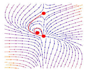
The critical points are locally stationary, which can be found by setting both the denominator and numerator to zero in (2.24a). There are three finite and three infinite critical points, each representing a different initial condition. The points at infinity represent different types of boundary conditions, including the flow of moving sinks, which is treated in Gratton & Minotti (1990), but unrelated to the inflow problem at hand. The finite critical points are

1. (i) $O:(H,U)=(0,0)$, the fluid is stationary and has constant height;

2. (ii) $A:(H,U)=(0,\delta )$, the current height is zero at the front and travels at a finite velocity, i.e. the advancing front of the viscous gravity current;

3. (iii) $B:(H,U)=[-3/2(5+3n),1/(5+3n)]$, the current height and velocity $h\propto (-x^2/t)^{1/3}$ and $u\propto x/t$ representing a flow outwards from the channel. Integration paths around point $B$ spiral endlessly, and so $U$ and $H$ exhibit oscillatory behaviour not found in the physical variables $u$ and $h$.

The flow to the origin is represented by the integral path from A to O, which only exists under specific values of $\delta (n)$. By finding $\delta (n)$, we can demonstrate the existence of a similarity solution of the second kind, and the actual flow can be simulated numerically using the phase plane.

The value of $\delta (n)$ can be found computationally by altering $n$ and changing the value of $\delta$ until the integral path shooting from perturbation at A reaches O, as seen in Zheng et al. (2014) and Zheng & Stone (2022). The generating perturbation to first order around point A can be found by linearising (2.24a), and the eigenvectors indicate which integral path passes through A. Let $\boldsymbol {r}_A\rightarrow \boldsymbol {r}_A + \delta \boldsymbol {r}$, where $\delta \boldsymbol {r}=(\eta,\mu )$, and consider up to the first order

(2.25)$$\begin{gather} \left.\frac{{\rm d} U}{{\rm d} H}\right|_A = \frac{\eta[3(1+n)(\delta +\mu)+2\delta -1]-3\mu(\delta+\mu)}{3\eta(2\eta+3\delta+3\mu)}\approx \frac{[(3n+5)\delta-1]\eta-3\mu\delta}{9\eta\delta}, \end{gather}$$

(2.26)$$\begin{gather}\delta\boldsymbol{r}\approx \begin{pmatrix} 9\delta & 0\\ (5+3n)\delta-1 & -3\delta \end{pmatrix} \boldsymbol{r}. \end{gather}$$

The eigenvectors corresponding to the linearised matrix are

(2.27a,b)$$\begin{gather} \lambda_1=9\delta,\quad \boldsymbol{e}_1= [12\delta,(5+3n)\delta-1]; \end{gather}$$

(2.28a,b)$$\begin{gather}\lambda_2=-3\delta,\quad \boldsymbol{e}_2=(0,1). \end{gather}$$

The integral paths are then created using the built-in Mathematica function NDSolve with an initial perturbation of the order of $10^{-3}$ along $\boldsymbol {e}_1$. The value of $\delta$ at different values of $n$ is then found by using the bisection method until the integration path passes the vicinity of O. Figure 7 shows part of the bisection method for $n=0.3$, where we see that a small difference in $\delta$ causes the trajectory to either be attracted towards B or shoot off to infinity.

Figure 7. To demonstrate the bisection method used to find $\delta _c$ for arbitrary $n$, we chose $n=1.5$ as an example of fluid flowing towards the origin. The critical points illustrated in this example are also present in different $n$, except the positions are scaled accordingly. The vector field represents the local variation of $(H,U)$, and the red line represents the integration path. Path A to O represents the inflow, so we change $\delta$ until the path connecting the two points appears. The upper half of the graph shows the behaviour of the integration path where $\delta$ is much higher or lower than the critical value $\delta _c$. The lower half is plotted with $\delta \rightarrow \delta _c$, which shows high sensitivity to changes in $\delta$. The path either enters a limit cycle around point B if $\delta <\delta _c$ or diverges towards infinity if $\delta >\delta _c$.

The instability shown in figure 7 is due to the imperfection of computational perturbation because $\delta \boldsymbol {r}$ is not infinitesimal. When $\delta <\delta _c$, the cycling path to B corresponds to an oscillation between $U$ and $H$, while $\delta >\delta _c$ shows that the fluid plunges into a sink at a finite distance. Both are divergent behaviours as the fluid converges and self-similarity breaks down as shown in Gratton & Minotti (1990).

Figure 8 shows the $\delta _c$ value obtained for various $n$ and the logarithmic plot, which proves to be approximately linear except in the region $n\rightarrow 0$. The value of $\delta (n)$ then decays exponentially towards $\delta _\infty =0.5$. Fitting the equation as

(2.29)\begin{equation} \delta(n) = a\,{\rm e}^{-kn}+\tfrac{1}{2}, \end{equation}

and using the FindFit function, we find

(2.30) \begin{align} \left.\begin{aligned} a & \approx 0.23,\\ k & \approx 0.30. \end{aligned}\right\} \end{align}

This result suggests similarity solutions of the second kind exist for most $n$ until the geometric assumptions breakdown. Especially, $n\rightarrow \infty$ introduces a straight edge at $x=1$, so the model breaks down at infinity, and the exact nature of the breakdown boundary requires further study. However, before the breakdown occurs, the geometry of the channel approximates to a wide wedge with the axisymmetric current flowing towards the origin with $\delta \rightarrow 1/2$. A comparison with the results of the ‘deep’ ($h\gg b$) case studied by Zheng et al. (2014) is presented in figure 9, which shows divergence behaviour as $n\rightarrow 1^-$ in the deep case, in contrast to no divergence in the shallow case up to the geometric breakdown. Recall the definition of the similarity variable $\eta =xt^{-\delta }$, scaling space $x\rightarrow ax$ has the same effect on the similarity variable as scaling time $t\rightarrow a^{-1/\delta }t$. Therefore, $\delta$ can be interpreted as the power between $x$ and $t$ to preserve the scale invariance, and a convergent $\delta$ implies the validity of the similarity method and therefore the scale invariance assumption. The similarity variable $\delta$ converges to $1/2$ in the shallow current case before geometric breakdown implies scaling equivalence between ‘stretching’ $x\rightarrow ax$ and ‘delaying’ measurement from release $t\rightarrow a^{-2}t$ as $n\gg 1$.

Figure 8. (a) The critical value of the self-similarity parameter $\delta _c$ for different power-law channels $n$. The data show a trend of asymptotic behaviour approaching $1/2$ as $n$ increases. (b) The best fit of 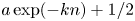$a\exp (-kn)+1/2$ together with $(n,\delta )$ data points on the logarithmic scale. The values of $a$ and $k$ were found numerically. There is a close agreement between the data and the linear trend line in the region of large $n$, and the model breaks down as $n\rightarrow 0$ due to the change of channel geometry beyond $n<1$.

Figure 9. Comparison between the similarity parameter $\delta$ when $h\gg b$ and $h\ll b$. The $h\gg b$ case studied by Zheng et al. (2014) shows a diverging trend approaching $n\rightarrow 1^-$, while the $h\ll b$ case has a similarity solution of the second kind for all $n$. Importantly, $\delta$ agrees for both cases at $n=0$.

3. Summary

We have investigated shallow viscous flows in a power-law channel ${\sim }x^n$ with $t^\alpha$ injection rate, considering both inflow and outflow, with possible application to models of different scales due to the scale invariance nature of the similarity solutions e.g. lava flow models and injection moulding. We showed that the outflow is described after some time by a similarity solution of the first kind and evaluated how long it takes for this similarity solution to be of the required accuracy compared with full numerical solutions. We found similarity solutions of the second kind for inflow in different $n$ channels using the numerical bisection method on the integration curve on the current phase plane. The similarity solutions of the second kind are determined by the similarity variable $\delta$, which decays exponentially to $\delta \rightarrow 1/2$ as the power of the channel increases, up until the breakdown of the geometric assumption. The parameter for the shallow current exhibits no divergent behaviour for $n\gg 1$, as opposed to the deep-current behaviour of the solutions in Zheng et al. (2014), possibly due to the breakdown of the deep-channel geometric assumption in the deep $n>1$ region, and requires further theoretical study to determine. The shallow-current result shows the validity of the similarity method to wider $n$ channels, which can produce asymptotic predictions on a large time scale. Experimental tests for the similarity solutions of the viscous gravity current are necessary to check the validity of the solutions in future work.