Hierarchical dose response of E. coli O157:H7 from human outbreaks incorporating heterogeneity in exposure

Summary

The infectivity of pathogenic microorganisms is a key factor in the transmission of an infectious disease in a susceptible population. Microbial infectivity is generally estimated from dose–response studies in human volunteers. This can only be done with mildly pathogenic organisms. Here a hierarchical Beta-Poisson dose–response model is developed utilizing data from human outbreaks. On the lowest level each outbreak is modelled separately and these are then combined at a second level to produce a group dose–response relation. The distribution of foodborne pathogens often shows strong heterogeneity and this is incorporated by introducing an additional parameter to the dose–response model, accounting for the degree of overdispersion relative to Poisson distribution. It was found that heterogeneity considerably influences the shape of the dose–response relationship and increases uncertainty in predicted risk. This uncertainty is greater than previously reported surrogate and outbreak models using a single level of analysis. Monte Carlo parameter samples (α, β of the Beta-Poisson model) can be readily incorporated in risk assessment models built using tools such as S-plus and @ Risk.

INTRODUCTION

Microbial risk assessment provides a scientific means for prospectively estimating the safety of foods and activities that determine human exposure to pathogenic microorganisms. Public trust in the scientific reliability of microbial risk assessment apparently is high, as various countries are developing legislation based on risk standards, e.g. regarding drinking water safety. Risk assessment has also been adopted as a means for safeguarding the public against the hazards associated with international trade of foodstuffs. In this area of ever-increasing implementation of risk assessment we need to extend and improve its scientific basis. One area of quantitative risk assessment which has received relatively modest attention is dose–response assessment. This is partly due to data restrictions, as dose–response assessment has so far been based on experimental studies, mostly on human volunteers or animal studies. For risk assessment of organisms where a dose–response relationship is not available, a surrogate dose–response relationship has been chosen, more or less arbitrarily. A surrogate could be either a pathogen with some similarity to the missing pathogen (e.g. Shigella for E. coli O157:H7 [1], with ID₅₀=1128), or a surrogate host (e.g. rabbits for E. coli O157:H7 [2], with ID₅₀=5·7×10⁵).

Incident or outbreak reports are often the first indication that any particular microorganism may be a health hazard. As such epidemiological reports deal with human patients with illness symptoms linked to exposure to some microbial hazard they can be considered prime evidence for the infectivity and/or pathogenicity of the pathogen at hand. Exposure is often not known quantitatively, but there are exceptions: sometimes food inspectors can obtain a sample of the implicated food and estimate the pathogen concentration. In a previous paper we investigated such an outbreak of E. coli O157:H7 in detail and could infer a dose–response relation [3].

However, a single outbreak provides limited information: usually the dose range is small, not several orders of magnitude as in experimental studies. Strachan et al. [4] collated data from eight different human outbreaks of E. coli O157:H7. These data showed considerable variation in observed attack rates, and a Beta-Poisson model could only be fitted by incorporating overdispersion in the form of a beta-binomial likelihood.

The observed variation between outbreaks is caused by many characteristics that may be different. The exposed population may differ, e.g. in age, or prior experience (acquired immunity to the pathogen); the vehicle may be different (different food, differences in preparation of the food); the pathogen may have a different history prior to its presence in the food. For such a meta-analysis a hierarchical model is appropriate, that can explicitly incorporate variation in infectivity between outbreaks.

In real world situations exposure cannot be assumed completely homogenous, as in experimental studies. The pathogen may be distributed unevenly in the vehicle (e.g. food or water) and the quantity ingested may also vary. This heterogenous exposure may thereby affect the dose–response relationship.

Here a hierarchical single-hit dose–response model is developed for outbreak data and compared with previously published models. The importance of heterogenous exposure is evaluated by its incorporation in the dose–response model.

OUTBREAK REPORTS

Table 1 lists numbers of exposed and affected subjects from eight different incidents, and estimated exposures in each case. Various transmission routes were implicated, including hand-to-mouth contamination, various foods, and water. Estimated exposure in these incidents covered a range of doses, from a few bacteria to 10 000 c.f.u.; attack rates ranged from 0·5% to 80%. Similar attack rates appear to correspond to different doses (sheep faces, hamburger) and similar doses correspond to different attack rates (salad sauce, salami), indicating heterogeneity in infectivity among incidents. In the following sections detailed descriptions of the outbreaks are given.

Table 1. Data from incidents involving E. coli O157:H7 (VTEC): vehicle, estimated dose, dispersion parameter, numbers exposed and infected and/or ill

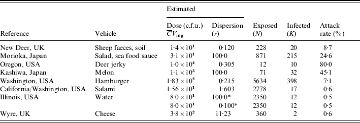
* Two scenarios: low and high dispersion.

Heterogeneity in exposure to microbial pathogens may be described by assuming any individual sample originating from a Poisson distribution with random parameters, for instance because of a varying concentration of the pathogens in the contaminated foodstuff, or because of a varying intake in exposed consumers. A Poisson-gamma mixture provides a simple and flexible model: individual exposure is negative binomial, while extra-Poisson variation is described by a single additional parameter, the shape parameter of the gamma component, henceforth called ‘dispersion’. Strong dispersion corresponds to clustered exposure: most consumers then ingested low doses, whereas few are likely to have ingested the majority of the pathogens present in the contaminated foodstuff.

For each of the outbreaks listed in Table 1 we have attempted to find a value for the dose (average number ingested) and the dispersion parameter (see Heterogenous inoculum section below). Avaliable information about the concentration of pathogens in ingested media was used. If microbial counts or presence–absence data were available maximum-likelihood methods were used. Alternatively, other statistics (average, quantiles) were used to calculate gamma distribution parameters. The same procedure was applied to describe consumed volumes. Then the product of the two gamma random variables (concentration and intake) was expressed as a single gamma distribution, by numerical approximation of average dose and dispersion. The following is a brief account of the available information for each outbreak, and the choices made in estimating parameters. Full information can be found in the listed references, particularly in Strachan et al. [4].

New Deer, UK

A scout camp, with 20 cases (out of 228). The probable route of E. coli O157 transmission was via hand contact with mud contaminated by sheep shedding E. coli O157. Strachan et al. [5] modelled the transfer of E. coli O157 from sheep to the soil and subsequently to humans and calculated an average dose of 14 c.f.u. Counts in soil samples collected on site showed strong dispersion, with an estimated dispersion parameter of 0·120.

Morioka, Japan

Contaminated school lunch resulting in 208 children and seven adults (out of 828 pupils and 43 teachers, respectively) infected with E. coli O157 [6]. Teunis et al. [3] estimated the average dose at 31 c.f.u. and argued that in this case there may have been little overdispersion. We therefore arbitrarily set the dispersion parameter at a value of 100·0.

Oregon, USA

Home-made venison jerky causing 10 cases from 12 exposed of gastroenteritis [7]. Cases had eaten 200 g on average, some had eaten more than 500 g (taken as 90th percentile of the gamma distribution describing the variation in intake). E. coli O157 was isolated from two leftover pieces of jerky, counts ranged from 3–93 c.f.u./g (used as 5th and 95th percentiles of the gamma distribution describing the variation in contamination). The distribution of the dose then is highly skewed, with a mean of 10 000 c.f.u. [4] and a dispersion parameter of 0·305.

Kashiwa, Japan

Contaminated melon eaten by 71 people resulted in 32 infected cases (28 children and four adults) [8]. The melon dish was found to contain 43 c.f.u./g E. coli O157 and it was estimated that about 1·1×10³ organisms were ingested by each person in a 25 g melon piece served per child. In the absence of any indication of overdispersion we assume Poisson inocula and set the dispersion parameter at 100.

Washington, USA

Major outbreak caused by undercooked contaminated ground beef patties at a chain of fast-food restaurants. In a prior risk assessment [9] the number of contaminated patties was estimated as 5634, accounting for underreporting, resulting in 398 primary cases [10]. Patties weighed 45 g. Taking into account that heating partially kills off these bacteria, it was estimated that the median dose was 23 c.f.u. [11]. Based on most probable number (mpn) the average number of organisms in a patty was 183. This is consistent with a dispersion parameter of 0·2.

California/Washington, USA

Consumption of dry fermented salami contaminated with E. coli O157 caused 17 cases of enteritis [12]. The consumed quantity was known for four cases, and ranged from 6–113 g. The total weight of the contaminated batch was 141 kg which, if consumed completely would cater for 2778 people exposed, assuming an average individual intake of 50 g salami. The concentration of E. coli O157 in recovered packages from retail was 0·3–0·4 c.f.u./g. Taking into account that both consumption and contamination are variable, we arrive at an average dose of 15·6 c.f.u., with an overall dispersion parameter of 1·603.

Illinois, USA

Waterborne outbreak, caused by swimming in water contaminated by E. coli O157. About 2350 people were exposed, and 12 cases were found [13]. The dose cannot be directly estimated but E. coli (not serotyped) were found in water taken a day before the incident. Based on the numbers counted and a presumed intake of 100 ml water [3] the average intake was estimated as 80 c.f.u. As we had no observations allowing estimates of the dispersion we studied two possibilities: low dispersion (dispersion parameter 100) and high dispersion (dispersion parameter 0·1).

Wyre, UK

Outbreak of E. coli O157 due to contaminated cheese. Two 9-kg cheeses were found to be contaminated with 5–10 c.f.u./g E. coli O157. It was established that two cases had consumed these contaminated cheeses. The total number exposed was unknown but assuming individual portions are 25–50 g, the two cheeses would represent 360 portions (if eaten completely). The mean dose has been estimated as 380 c.f.u. [4]. Using dispersion estimates for both concentration of bacteria and consumed portions, the overall dispersion could be estimated as 11·23.

HIERARCHICAL DOSE–RESPONSE MODEL WITH HETEROGENOUS DOSE

Poisson inoculum

For a Poisson inoculum the probability of exposure is

where C is the pathogen concentration and V _ing the ingested volume.

When infection results from independent action of ingested pathogens, and any pathogen survives (m) host barriers with probability p _m, the probability of infection is

This is the hit theory model for microbial dose response [14] which can be used to estimate infectivity of a single infectious unit.

Illness is conditional on infection. Often, asymptomatic infections may be present in outbreaks, but analysis for their detection is not usually performed. We therefore make the pragmatic assumption that the conditional probability of becoming ill when infected is 1, implying that infection predicted by the dose–response model corresponds to illness.

Heterogenous inoculum

For a negative binomial inoculum, when overdispersion is modelled as a Poisson-gamma mixture the probability of exposure is

where is the average concentration, and r is the dispersion parameter (shape parameter of the gamma-distributed microbial concentration).

And a fixed single-hit probability p _m results in a probability of infection

Heterogenous host–pathogen interaction

Heterogeneity in p _m is usually represented by a beta distribution g(p _m|α, β). The probability of infection is then a mixture

which can be integrated to yield the confluent hypergeometric function (₁F ₁)

The latter approximation holds for α≪β; β≫1. This is the well known Beta-Poisson dose–response model†. Alternately, in case of heterogenous exposure

which integrates to obtain the following hypergeometric function (₂F ₁).

Statistical analysis

The hierarchical framework for the parameters of the Beta-Poisson dose–response model is given in Figure 1. The two levels of the model are represented by two nested loops. The inner loop describes the dose–response relation for each individual outbreak, described by the parameter pair (α(j), β(j)). The outer loop represents variation among the separate outbreak dose–response relations, described by the (joint) distribution of α and β, with (hyper-)parameters (ρ_α, λ_α), (ρ_β, λ_β). The likelihood is binomial: for each outbreak k(j,) cases out of n(j,) people exposed to a dose CV _ing(j) have been observed.

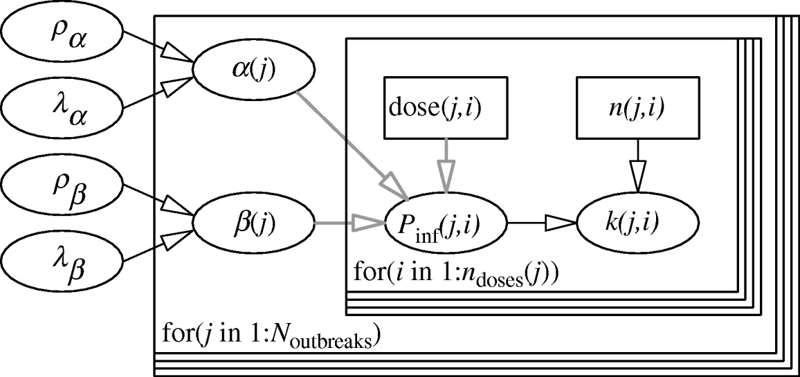
Fig. 1. Two-level model for dose–response assessment of several outbreaks, each with their separate pathogen isolates and possible susceptibility distributions. Inner loop: dose groups within outbreaks, i=1, …, n _doses (j); Outer loop: outbreaks, j=1, …, N _outbreaks. (Note that here n _doses (j)=1 for all outbreaks.)

Parameters are transformed as in Teunis et al. [3]: since we have only one data-point per outbreak, the parameters (α, β) of the Beta-Poisson model are highly correlated: parameter estimation is improved by transformation to

(1)

so that we are estimating the mean value (u) of the beta distribution for p _m and a quantity that is inversely related to its variance (for very large positive values of v the variance tends to zero). Further u is logit-transformed and v is log-transformed

(2)

We use normal priors for w and z (mean ρ, standard deviation λ). Uncorrelated non-informative normal (−8, 8) hyper-priors were taken for the means of w and z (ρ), gamma (0·001, 1000) priors were taken for the standard deviations of w and z (λ).

Note that the dispersion parameter r is given, estimated from the analysis of exposure conditions (see Table 1). Posterior parameter samples have been obtained using the Metropolis–Hastings algorithm, implemented in Mathematica [3].

Predictions of infectivity may be obtained by sampling from the posterior (joint) distributions of hyper-parameters ((ρ_α, λ_α), (ρ_β, λ_β) in Fig. 1). This can be done by adding an outbreak consisting entirely of missing data, thereby omitting the inner loop of the model and causing the Markov chain Monte Carlo (MCMC) algorithm to sample only from the joint distributions of (α( ), β( )). With such a procedure prediction is equivalent to assuming that the infectivity of any unknown VTEC isolate is a sample of the infectivity ‘universe’ defined by the set of outbreaks used here.

RESULTS

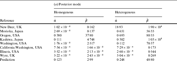
Hierarchical dose–response models were developed for the two scenarios: homogenous exposure for all outbreaks and heterogenous exposure (Illinois, USA: two possible alternatives; see Outbreak reports section 2). Figure 2 shows approximated (by MCMC) posterior mode dose–response relations for each of the eight incidents to illustrate the contribution of each outbreak to the estimated variation in infectivity. These curves were obtained by calculating the joint posterior (partial) probability for each iteration in the Markov chain and taking the sample with the highest value.

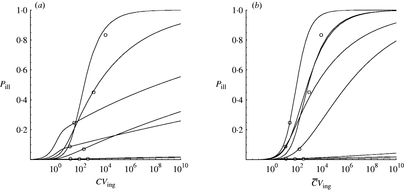
Fig. 2. Posterior mode (approximated from MCMC) dose–response curves for the outbreak data in Table 1. (a) Homogenous exposure; (b) heterogenous exposure.

Figure 3 shows percentile contours of the group dose–response relation, generated from the individual dose–response models in Figure 2. These were obtained by sampling from the prior distributions for w and z (and, indirectly, α and β).

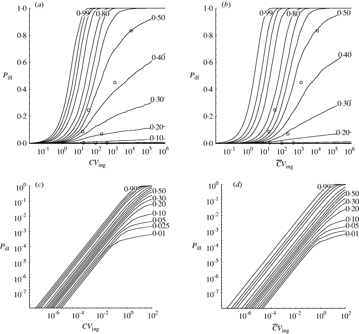
Fig. 3. Contour chart of predicted percentiles of dose–response relation for the outbreak data in Table 1 (a) (c, d) Extrapolated to low doses (log-log graph). (a, c) Homogenous exposure; (b, d) heterogenous exposure.

Compared to the homogenous model, the heterogenous one appears not to indicate strongly different infectivity, but does show increased uncertainty, as visualized by the wider percentile contours. This is particularly clear for low-dose extrapolations [Fig. 3 (c, d)].

Figure 4 shows the probability density of the single-hit probability p _m for both homogenous and heterogenous models. An infection risk of a few percent (1–10%) for a single ingested organism appears quite probable. Interestingly, the heterogenous model appears to result in a lower variability (narrower distribution) in p _m compared to the homogenous case. Key statistics for the models are presented in Table 2.

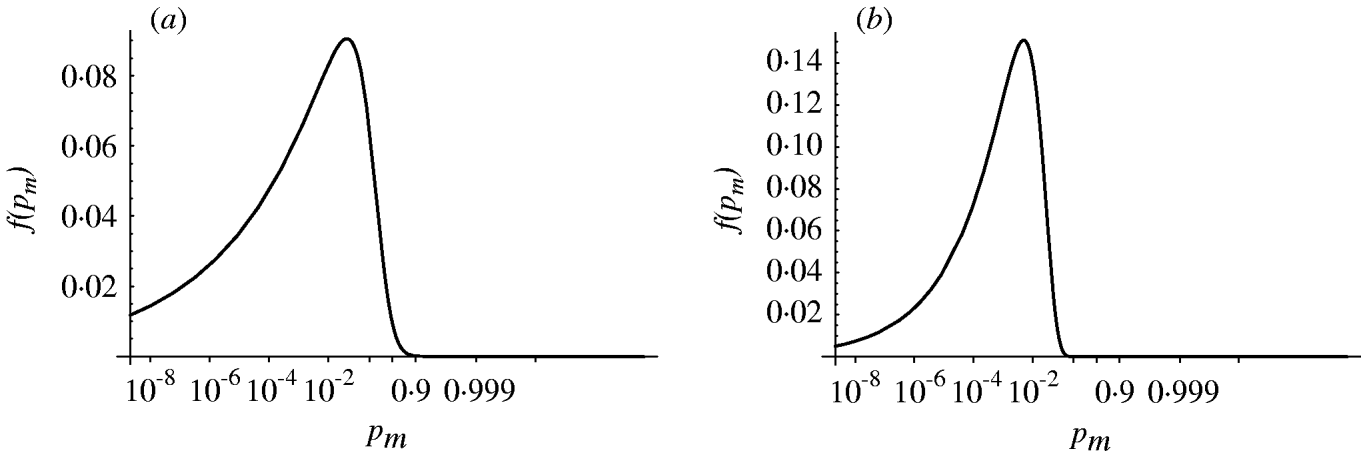
Fig. 4. Probability density of the single-hit probability of infection p _m (transformed to a logit scale). (a) Homogenous exposure; (b) heterogenous exposure.

Table 2. (a) Parameter values for the ‘best fit’ (posterior mode) curves of the separate outbreaks (cf. Fig. 2) and the predicted group dose–response model (prediction). (b) Statistics for the Monte Carlo sample of predictive parameter values: 5, 50 and 95 percentiles, and correlation coefficient

DISCUSSION

The dose–response models in this paper were used to analyse outbreak data in a hierarchical framework. This may be called a meta-analysis. The variation in apparent infectivity among outbreaks is interpreted as a biological property, i.e. as heterogeneity within and between outbreaks. From this the dose–response relation for each of the individual outbreaks presented can be generalized to the group level. In doing this the variation that is potentially present in all unobserved outbreaks with the same pathogen is incorporated. This can be seen from the appropriate coverage displayed in Figure 3.

Variation in the probability of (symptomatic) infection may have many different causes: variation in susceptibility of the exposed population, intrinsic pathogen properties (e.g. genetic variation), condition of the pathogen (e.g. survival in the food matrix or water, temperature, previous hosts). The dose–response model cannot discriminate between these different sources of heterogeneity because they are individually unidentifiable. If detailed information on the condition of the pathogen or, for example, the immune status of the exposed population was available, this might allow adaptation of the model to incorporate such sources of variation [15].

Strachan et al. [4] collated the outbreak data used here and demonstrated a dose–response model could be built. However, variability between outbreaks could only be incorporated when using a beta-binomial likelihood. This model agrees with the hierarchical model for median and upper (95%) percentiles but underestimates the lower (5%) level of risk where some of the outbreak data-points lie.

When compared to the predictions based on only the Morioka outbreak, as shown in a previous paper [3] it is clear that the predictions presented in the current paper show less uncertainty. Moreover, the strain of E. coli O157 from the Morioka outbreak appears to be highly infectious compared to most other outbreaks.

Recapitulating the findings of Strachan et al. [4] the Shigella model [1] is contained within the predicted risk interval. The lower (5%) percentile contour of the dose–response envelope developed by Powell et al. [16] more or less coincides with those in Figure 3, whereas the upper (95%) levels are underestimated, even more so than in [4]. The rabbit model [2] underestimates the human risk of E. coli O157.

Dose–response models are affected by heterogeneity both in exposure and in infectivity. Complete absence of heterogeneity results in an exponential dose–response relation. Any increase in heterogeneity results in a less steep dose–response relation. We have modified the dose–response model to include non-Poisson exposure. As both sources of heterogeneity act the same on the shape of the dose–response relation, they cannot usually be identified when fitting the model to dose–response data. However, a priori information on the dispersion of the inoculum is available, which leaves the remaining heterogeneity to be attributed to infectivity.

For a given slope, obtained by fitting the model to data, there is a trade-off between heterogeneity in exposure (which has been specified in this paper) and also heterogeneity in infectivity. This means that higher dispersion in exposure results in a narrower distribution of the infectivity p _m. In other words: given the dose–response data the estimated infectivity depends on the choices made for dispersion in exposure. This emphasizes the importance of knowledge about the dose: not only its magnitude, but also its heterogeneity (dispersion), to obtain unbiased estimates of infectivity.

The outbreaks detailed here show considerable variation in apparent infectivity: at low c.f.u. doses high responses are observed in some cases, other cases, however, appear to have low attack rates at much higher doses. For this reason a second level of analysis is necessary: variation among outbreaks. The observed variation among outbreaks may involve differences in pathogen conditions, pathogen–host interactions, and even intake behaviour. We cannot discriminate between such different causes, and only use the hierarchical statistical model as a shorthand description of this complex problem.

The data used in this analysis comprise symptomatic cases, as only these can be detected, especially when a large population is exposed, as in the Washington beefburger outbreak [10]. Strictly speaking the Beta-Poisson model is an infection dose–response model where infection does not necessarily imply illness. In general, asymptomatic infections may occur, perhaps reflecting natural variation in susceptibility among hosts [17]. In applying the Beta-Poisson model to outbreak data, infection is assumed to imply illness, at sufficiently high doses. For a highly virulent pathogen like E. coli O157:H7 this seems reasonable.

Most microbial dose–response information has been obtained in clinical studies, selecting only mildly pathogenic organisms, usually propagated in laboratory conditions, excluding risk groups from the volunteer population. In contrast, studying outbreaks selects for highest pathogenicity, with pathogens propagated under ‘natural’ conditions, and preference for susceptible groups in the host population. The dose–response relation in Figure 3 therefore may represent a ‘worst case’ situation. Not all strains of E. coli O157:H7 may be equally pathogenic, therefore some outbreaks may remain undetected. However, it seems plausible that most outbreaks are detected because the most susceptible subjects in the exposed population become ill. The attack rate for illness therefore may be lower for some strains (or foodstuffs, or host populations), but some illness cases are still observed, and the apparent low pathogenicity is interpreted as increased heterogeneity in infectivity.

In absence of human dose–response information for the pathogen of concern surrogate information can be used: the same pathogen in surrogate hosts, or a (presumed) similar pathogen for which human dose–response data are available.

In toxicology animal models have been employed as surrogates for human dose response and in analogy several studies of human pathogens in various animals have been published. Such studies may provide useful insights into the mechanisms of microbial infection and pathogenesis but their significance for risk assessment remains uncertain. Most studies deal with gastrointestinal pathogens. Although some studies use primates or piglets, for ease of use mostly rodents are used, and it is doubtful whether intestinal infection or illness in rats may be compared qualitatively to intestinal infection or illness in humans.

One of the main aims of risk assessment is making quantitative predictions, which may be considered speculative if based on animal dose–response data. This is illustrated by the considerable discrepancy between human and rabbit dose response for E. coli O157:H7 [2].

The parameters produced by the hierarchical dose–response model can be readily used in risk assessment. A Monte Carlo sample of (α, β) pairs can be incorporated into a range of popular risk tools. These parameters represent variation in infectivity which is host–pathogen specific but not exposure which is dependent on the specific outbreaks used to generate the model, and were accounted for by the dispersion estimates. These sets of parameter pairs (α, β) can be obtained from the authors.

The predictive intervals in Figure 3 (a, b) at high doses seem quite wide compared to most previously published single-level models. But at low doses [Fig. 3 (c, d)] predictive intervals are fairly narrow due to the high infectivity of E. coli O157:H7 [3].

CONCLUSIONS

Outbreak data can be used for setting up dose–response models for microbial pathogens. It is, however, critical to allow for additional variability, compared to controlled clinical studies: variation in infectivity at the level of the individual host as well as variation between outbreaks, and heterogeneity in exposure. If heterogenous exposure can be quantified its influence on the dose–response relationship can be incorporated to correct infectivity estimates.

Outbreak data as used here are exceedingly rare in the published literature even though relatively many outbreaks occur. There is a need for more outbreak data to further validate this model and to generate corresponding models for other pathogens of public health concern. This need is exacerbated due to the ethical concerns associated with human feeding studies. Only when such information becomes available can a suite of dose–response models be generated, resulting in more valid quantitative risk assessments.