


1. Introduction
The study of passive scalars within wall-bounded turbulent flows is of significant practical importance. It has relevance in understanding the behaviour of diluted contaminants and serves as a model for the temperature field under the assumption of low Mach number and small temperature differences (Monin & Yaglom Reference Monin and Yaglom1971; Cebeci & Bradshaw Reference Cebeci and Bradshaw1984). However, measuring the concentration of passive tracers and small temperature differences is challenging, resulting in limited information about even basic passive scalar statistics (Gowen & Smith Reference Gowen and Smith1967; Kader Reference Kader1981; Subramanian & Antonia Reference Subramanian and Antonia1981; Nagano & Tagawa Reference Nagano and Tagawa1988).
The understanding of passive scalars in turbulent flow primarily focuses on the case where the Prandtl number ( ${{Pr}}$) is approximately equal to 1. The Prandtl number represents the ratio of kinematic viscosity to thermal diffusivity (
 ${{Pr}}=\nu /\alpha$). Several studies have verified the close analogies between the passive scalar field and the longitudinal velocity field in this case (Kim, Moin & Moser Reference Kim, Moin and Moser1987; Abe & Antonia Reference Abe and Antonia2009; Antonia, Abe & Kawamura Reference Antonia, Abe and Kawamura2009). However, many fluids, such as water, engine oils, glycerol and polymer melts, have Prandtl numbers significantly higher than unity, whereas liquid metals and molten salts can have much lower Prandtl numbers. In the case of diffusion of contaminants, the role of the Prandtl number is taken by the Schmidt number, which represents the ratio of kinematic viscosity to mass diffusivity. The typical values of the Schmidt number in applications are always much higher than unity (Levich Reference Levich1962). Under these circumstances, the similarity between velocity and passive scalar fluctuations is substantially impaired, making predictions of even the basic flow properties quite challenging.
Concerning wall fluxes, the most robust framework established so far is the work of Kader & Yaglom (Reference Kader and Yaglom1972). Based on universality arguments, those authors derived a predictive law for the non-dimensional flux (Nusselt number) as a function of the Prandtl number. This framework mainly requires modelling the logarithmic offset function, which is the Prandtl-dependent additive constant in the overlap-layer mean passive scalar profiles. Despite this solid framework, semiempirical power-law correlations (Dittus & Boelter Reference Dittus and Boelter1933; Kays, Crawford & Weigand Reference Kays, Crawford and Weigand1980) are still widely used in engineering design. Regarding the mean profiles of passive scalars, the most detailed study dates back to Kader (Reference Kader1981), who derived an empirical interpolation formula that connects the universal near-wall conductive layer with the outer logarithmic layer. This interpolation formula was found to agree reasonably well with the observed behaviour of the temperature profile in experiments available at that time.
Pirozzoli (Reference Pirozzoli2023) studied the statistics of passive scalars in pipe flow in the range of Prandtl numbers from  ${{Pr}}=0.00625$ to
  ${{Pr}}=16$, using direct numerical simulation (DNS) of the Navier–Stokes equations, and found that the mean passive scalar profiles at
  ${{Pr}} \gtrsim 0.0125$ exhibit logarithmic overlap layers, and universal parabolic distributions in the core part of the flow. A model of the eddy viscosity was used to derive semianalytical predictions (numerical quadrature was required) for the mean passive scalar profiles, and for the corresponding logarithmic offset function. Asymptotic scaling formulae were also derived for the thickness of the diffusive sublayer and the heat transfer coefficient, which are capable of accounting accurately for variations with both the Reynolds and the Prandtl numbers, for
  ${{Pr}} \gtrsim 0.25$. In this paper, we use the same DNS database, with the goal of deriving fully explicit analytical representations for the mean passive scalar profiles and the corresponding wall fluxes as functions of the Reynolds and Prandtl numbers. Although, as previously pointed out, the study of passive scalars is relevant in several contexts, one of the primary fields of application is heat transfer, and therefore from now on we will refer to the passive scalar field as the temperature field (denoted as
  $T$), and passive scalar fluxes will be interpreted as heat fluxes.
2. The numerical dataset
Numerical simulations of fully developed pressure-driven turbulent flow in a circular pipe are carried out at bulk Reynolds number  ${{Re}}_b\ (= 2 R u_b / \nu ) = 44\,000$, with
  $R$ the pipe radius,
  $\nu$ the fluid kinematic viscosity and
  $u_b$ the bulk velocity, corresponding to friction Reynolds number
  ${{Re}}_{\tau }\ ( = u_{\tau } R / \nu ) \approx 1140$, with
  $u_{\tau } = (\tau _w/\rho )^{1/2}$ the friction velocity,
  $\rho$ the fluid density and
  $\tau _w$ the wall shear stress. Periodic boundary conditions are assumed along the axial (
 $z$) and azimuthal (
 $\phi$) directions. The incompressible Navier–Stokes equations are augmented with the transport equation for a passive scalar field (buoyancy effects are disregarded), with different values of the thermal diffusivity (hence, various
  ${{Pr}}$), and with isothermal boundary conditions at the pipe wall (
 $r=R$).
The computer code has been described in previous publications (Pirozzoli et al. Reference Pirozzoli, Romero, Fatica, Verzicco and Orlandi2022), and the DNS database herein considered was presented in detail in a separate publication (Pirozzoli Reference Pirozzoli2023). A list of the main simulations that we have carried out is provided in table 1. Eleven values of the Prandtl number are considered, from  ${{Pr}} = 0.00625$ to
  $16$. Note that a finer mesh is used for flow cases with
  ${{Pr}} > 1$, so as to satisfy restrictions on the Batchelor scalar dissipative scale, whose ratio to the Kolmogorov scale is about
  ${{Pr}}^{-1/2}$ (Batchelor Reference Batchelor1959; Tennekes & Lumley Reference Tennekes and Lumley1972).
Table 1. Flow parameters for DNS of pipe flow at various Prandtl numbers. Here  $N_z$,
  $N_r$ and
  $N_{\phi }$ denote the number of grid points in the axial, radial and azimuthal directions, respectively;
  ${{Pe}}_{\tau } = {{Pr}} \, {{Re}}_{\tau }$ is the friction Péclet number;
  ${{Nu}}$ is the Nusselt number (as defined in (3.19)); and # ETT is the time interval considered to collect the flow statistics, in units of the eddy-turnover time, namely
  $R/u_\tau$. For all DNS,
  $L_z = 15 R$,
  ${{Re}}_b=44\,000$ and
  ${{Re}}_{\tau }=1137.6$.

From now on, inner normalization of the flow properties will be denoted with the ‘ $+$’ superscript, whereby velocity is scaled by
  $u_{\tau }$, wall distance (
 $y=R-r$) by
  $\nu /u_{\tau }$ and temperature by the friction temperature,
 \begin{equation} T_{\tau} = \frac{\alpha}{u_{\tau}} \left\langle \frac {\mathrm{d} {T}}{\mathrm{d} y} \right\rangle_w, \end{equation}
where angle brackets denote averaging in the homogeneous spatial directions and in time, and the subscript  $w$ denotes wall properties. In particular, let
  $\theta = T-T_w$; then the inner-scaled temperature is defined as
  $\theta ^+ = \theta /T_{\tau }$. Hereafter capital letters will be used to denote averaged flow properties, and lower-case letters to denote fluctuations from the mean.
3. Analysis
3.1. Mean profiles
Modelling the turbulent heat fluxes requires closures with respect to the mean temperature gradient (see e.g. Cebeci & Bradshaw Reference Cebeci and Bradshaw1984) through the introduction of a thermal eddy diffusivity, defined as
 \begin{equation} \alpha_t = \frac{\langle u_r \theta \rangle}{\mathrm{d} \varTheta / \mathrm{d} y}. \end{equation}
 Figure 1 shows that the turbulent thermal diffusivities inferred from the DNS data have a rather simple behaviour. Figure 1(a) shows the near-collapse of all cases to a common distribution, with the reminder that a log–log scale is used to better bring out the near-wall behaviour. Cases with  ${{Pr}} \lesssim 0.125$ fall outside the universal trend, as they show a similarly shaped distribution of
  $\alpha _t$, but lower absolute values. In fact, universality in the zero-Prandtl-number limit cannot be expected, as the turbulent heat flux must eventually vanish. In agreement with asymptotic arguments (Kader & Yaglom Reference Kader and Yaglom1972), the limiting near-wall behaviour is
  $\alpha _t \sim y^3$. Farther from the wall, there is evidence for a narrow region with linear growth of
  $\alpha _t$, as would be the case in the presence of a sizeable logarithmic layer. As a reference, the distribution of
  $\alpha _t$ at
  ${{Re}}_{\tau }=6000$ and
  ${{Pr}}=1$ is also reported (black dotted line), which shows that, indeed, the linear region becomes wider at higher
  ${{Re}}$. The distributions of
  $\alpha _t$ in the near-wall and logarithmic regions can be closely modelled using a suitable functional expression, which we assume to have the same structure as the eddy viscosity considered by Musker (Reference Musker1979), namely
 \begin{equation} \alpha_t^+= \frac{(k_{\theta} {y^+})^3}{(k_{\theta} {y^+})^2+C_{\theta}^2}, \end{equation}
where  $k_{\theta } \approx 0.459$ (Pirozzoli et al. Reference Pirozzoli, Romero, Fatica, Verzicco and Orlandi2022), which has the proper asymptotic behaviours
 \begin{gather} \alpha_t^+ \stackrel{y^+ \to 0}{\approx} {y^+}^3/C_{\theta}^2, \end{gather}
 \begin{gather}\alpha_t^+ \stackrel{y^+ \to \infty}{\approx} k_{\theta} y^+. \end{gather}
Figure 1. Distributions of inferred eddy thermal diffusivity ( $\alpha _t$) as a function of wall distance. In (a) the black dotted line denotes
  $\alpha _t$ for the case
  ${{Re}}_{\tau }=6000$, at
  ${{Pr}}=1$ (Pirozzoli et al. Reference Pirozzoli, Romero, Fatica, Verzicco and Orlandi2022), and the grey dashed lines denote the asymptotic trends
  $\alpha _t^+ \sim {y^+}^3$ towards the wall and
  $\alpha ^+_t = k_{\theta } y^+$ in the log layer (
 $\alpha _t^+ = \alpha /\nu$). In(b) the dash-dotted line denotes the fit given in (3.2). Colour codes are as in table 1.
Figure 1(b) shows that (3.2) with  $C_{\theta }=10.0$ yields a nearly perfect fit of the DNS data, with slight deviations at
  $y^+ \lesssim 10$, where in any case the eddy diffusivity is much less than the molecular one. Whereas alternative functional expressions are possible (Pirozzoli Reference Pirozzoli2023), (3.2) bears the substantial advantage of being amenable to further analytical developments.
Starting from the (once-integrated) mean thermal balance equation,
 \begin{equation} \frac 1{{\it Pr}} \frac{\mathrm{d} \varTheta^+}{\mathrm{d} y^+} + \langle u_r \theta \rangle^+= 1 - \frac{y^+}{{\it Re}_{\tau}}, \end{equation}
and under the inner-layer approximation ( $y^+/{{Re}}_{\tau } \ll 1$), one can in fact infer the distribution of the mean temperature in the inner layer from knowledge of the eddy thermal diffusivity, by integrating
 \begin{equation} \frac{\mathrm{d} \varTheta^+}{\mathrm{d} y^+} = \frac {{\it Pr}}{1 + {\it Pr} \, \alpha_t^+}, \end{equation}
with  $\alpha _t$ given in (3.2). The result of the integration is
 \begin{align} \varTheta^+ &= \frac{1}{2 k_{\theta} \eta_0 (2 + 3 {\it Pr}\,\eta_0)} \bigg\{\frac {2( 2 \eta_0 + 3 {\it Pr}^2 C_{\theta}^2 \eta_0 + {\it Pr} (C_{\theta}^2+2 \eta_0^2) )}{\varDelta} \bigg[\arctan{\left( \frac{1+{\it Pr}\,\eta_0}{\varDelta} \right)} \nonumber\\ &\quad - \arctan{\left( \frac{1+{\it Pr} (2 \eta + \eta_0)}{\varDelta} \right)}\bigg] + 2 {\it Pr} ( C^2 + \eta_0^2 ) \log \left(1-\frac{\eta}{\eta_0}\right) \nonumber\\ &\quad + ( {\it Pr} (2 \eta_0^2 - C_{\theta}^2 ) + 2 \eta_0 ) \log{\left(\frac{{\it Pr} \,\eta^2 + (1 + {\it Pr} \,\eta_0)(\eta+\eta_0)}{\eta_0 (1 + {\it Pr} \,\eta_0)}\right)}\bigg\}, \end{align}
where  $\eta =k_{\theta } y^+$,
  $\varDelta = (3 {{Pr}}^2 \eta _0^2 + 2 {{Pr}}\, \eta _0 -1)^{1/2}$ and
  $\eta _0$ is the single (negative) real root of the cubic equation
 \begin{equation} {\it Pr}\,\eta^3 + \eta^2 + C_{\theta}^2 = 0, \end{equation}
whose exact solution is
 \begin{equation} \eta_0 = \frac 1{3 {\it Pr}} \left( - 1 + \frac 1z + z \right),\quad z= \left[ \frac 12 \left({-}2 - 27 {\it Pr}^2 C_{\theta}^2 + \sqrt{-4+ ( 2 + 27 {\it Pr}^2 C_{\theta}^2 )^2} \right) \right]^{1/3} . \end{equation}
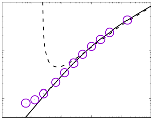
 As figure 2 clearly shows, the quality of the resulting reconstructed temperature profiles is generally very good, with obvious deviations of the outermost region of the flow, which is not covered by the present analysis, but which could be easily accounted for based on outer-layer universality arguments (Pirozzoli Reference Pirozzoli2023). Deviations from the predicted trends are observed at the lowest Prandtl numbers ( ${{Pr}} \lesssim 0.125$), which, as previously noted, deviate from the universal trend of
  $\alpha _t$. The quality of the interpolation formulae provided by Kader (Reference Kader1981, equation (9), symbols) is overall also good. However, the behaviour in the buffer layer is somewhat unnatural, and the log-law offset seems to be a bit overestimated.

Figure 2. (a) Comparison of mean temperature profiles obtained from DNS (solid lines), with the predictions of (3.6) (dashed lines) and with Kader's (Reference Kader1981) empirical fit (circles). (b) A magnified view to emphasize the behaviour of the low- ${{Pr}}$ cases.
The solution in (3.8a,b) is not particularly convenient for further developments, and it is tricky to implement numerically, as it suffers from severe cancellation problems at high  ${{Pr}}$. A much more convenient approximation will be exploited in the following analysis, based on its expansion in powers of the Prandtl number, which returns the following:
 \begin{equation} \eta_0 ={-} \frac 1{3 {\it Pr} \,\chi} ( 1 + \chi + \chi^2 ) + O(\chi^2),\quad \chi= \frac{( C_{\theta} {\it Pr} )^{{-}2/3}}3 . \end{equation}
The quality of this approximation can be judged from figure 3(a), which shows deviations of less than  $1\,\%$ for
  ${{Pr}} \gtrsim 0.1$.

Figure 3. (a) Comparison of the root of (3.7),  $\eta _0$, as obtained from (3.8a,b) (solid line) and from the asymptotic solution (3.9a,b) (dashed line). The inset shows the relative deviation of the latter from the former. (b) The predicted thickness of the conductive sublayer (
 $\delta _{t}^+ = - \eta _0/k_{\theta }$) with the exact formula and with the asymptotic approximation, compared with the DNS data (solid symbols), in which
  $\delta _t$ is estimated from equality of turbulent and conductive heat flux.
An important property to define the behaviour of passive scalars in wall-bounded flows is the thickness of the conductive sublayer. The latter has been given several definitions (see e.g. Levich Reference Levich1962; Schwertfirm & Manhart Reference Schwertfirm and Manhart2007; Alcántara-Ávila & Hoyas Reference Alcántara-Ávila and Hoyas2021). However, we believe that the most obvious is the wall distance at which the turbulent heat flux equals the conductive one, which, based on (3.4), occurs when
 \begin{equation} \alpha_t^+ (\delta_{t}^+) = \frac 1{\it Pr} . \end{equation}
Assuming the validity of the closure (3.2), we find that  $\delta _{t}$ must satisfy the cubic equation
 \begin{equation} {\it Pr} (k_{\theta} {\delta_{t}^+})^3 - (k_{\theta} {\delta_{t}^+})^2 - C_{\theta}^2 = 0, \end{equation}
hence  $\delta _{t}^+ = - \eta _0/k_{\theta }$. Figure 3(b) shows that this is an excellent approximation of the DNS data, both when the ‘exact’ formula in (3.8a,b) is used for
  $\eta _0$, and when the expansion given in (3.9a,b) is used instead, again with deviations at low Prandtl number.
As shown in figure 2, the inner-layer mean temperature distributions at  ${{Pr}} \gtrsim 0.0125$ exhibit a near-logarithmic behaviour, namely
 \begin{equation} \varTheta^+= \frac 1{k_{\theta}} \log y^+ + \beta ({\it Pr}), \end{equation}
where  $\beta$ is a Prandtl-dependent offset, whose role is crucial in the estimation of the heat transfer coefficient (see below). The function
  $\beta ({{Pr}})$ can be determined by taking the limit
 \begin{equation} \beta({\it Pr}) = \lim_{y^+ \to \infty} \left( \varTheta^+ (y^+) - \frac 1{k_{\theta}} \log y^+ \right), \end{equation}
which, exploiting (3.6), yields
 \begin{align} \beta({\it Pr}) &= \frac{1}{2 k_{\theta} \eta_0 (2 + 3 {\it Pr}\,\eta_0)} \bigg\{\frac {2( 2 \eta_0 + 3 {\it Pr}^2 C_{\theta}^2 \eta_0 + {\it Pr} (C_{\theta}^2+2 \eta_0^2) )}{\varDelta} \nonumber\\ &\quad \times\left[\arctan{\left( \frac{1+{\it Pr}\,\eta_0}{\varDelta} \right)}-\frac{\rm \pi}2\right] - 2 {\it Pr} ( C^2 + \eta_0^2 ) \log (-\eta_0) \nonumber\\ &\quad +( {\it Pr} (2 \eta_0^2 - C_{\theta}^2 ) + 2 \eta_0 ) \log{\left(\frac{{\it Pr}}{\eta_0 (1 + {\it Pr}\,\eta_0)}\right)}\bigg\} + \frac 1{k_{\theta}} \log{k_{\theta}}. \end{align}
 Whereas (3.14) is very accurate, it does not clearly highlight trends with the Prandtl number. A much simpler and equally accurate formula can then be derived by exploiting (3.9a,b), and expanding all terms in (3.14) in powers of the parameter  $\chi$. After lengthy developments, the final result is
 \begin{align} \beta({\it Pr}) &= \frac 1{k_{\theta}} \left[ \frac{2 {\rm \pi}C_{\theta}^{2/3}}{3 \sqrt{3}} {\it Pr}^{2/3} + \frac 13 \log {\it Pr} - \left( \frac 16 + \frac 1{2 \sqrt{3}} + \frac 23 \log C_{\theta} - \log k_{\theta} \right) \right] \nonumber\\ &\quad + O({\it Pr}^{{-}2/3}). \end{align}
With the assumed numerical values of the constants  $k_{\theta }\ (=0.459)$ and
  $C_{\theta }\ (=10.0)$, (3.15) becomes
 \begin{equation} \beta({\it Pr})= 12.2 {\it Pr}^{2/3}+ 0.726 \log {\it Pr}- 6.03 . \end{equation}
 It is remarkable that a structurally identical formula in terms of  ${{Pr}}$ dependence was arrived at by Kader & Yaglom (Reference Kader and Yaglom1972, equation (28)) based on a crude three-layer eddy conductivity model, which led to
 \begin{equation} \beta({\it Pr})=12.5 {\it Pr}^{2/3} + 2.12 \log {\it Pr} - 5.3. \end{equation}
In this equation, the coefficient in front of the logarithmic term was determined analytically to be  $1/k_{\theta }$ (with
  $k_{\theta } = 0.47$, hence a bit different than the present), and thus fundamentally different than in (3.15), where the prefactor of the logarithmic term is
  $1/(3 k_{\theta })$. Furthermore, the prefactor of the first term and the trailing additive constant in (3.17) were determined empirically, by matching the experimental data available at that time. Equation (3.15) bears the clear advantage that values of all coefficients are given explicitly, as a function of the single parameter
  $C_{\theta }$, which we determined once and for all by fitting the distributions of the eddy diffusivity inferred from the DNS. All the rest of the expression is determined analytically.
The variation of the logarithmic offset function with  ${{Pr}}$ is examined in figure 4. In figure 4(a) we illustrate the procedure that we have followed in order to obtain estimates of
  $\beta ({{Pr}})$, based on fitting the mean temperature distributions obtained from DNS with (3.12). Near-logarithmic distributions are recovered for all cases, with the exclusion of the
  ${{Pr}}=0.00625$ case. Figure 4(b) then compares the log-law offset constant inferred from the DNS temperature profiles with the prediction of (3.15) and with (3.17). The superiority of the former is quite clear, as (3.15) yields an excellent approximation of
  $\beta$ even at
  ${{Pr}} \ll 1$, where it is not expected to work well. As admitted in the original reference, the formula developed by Kader & Yaglom (Reference Kader and Yaglom1972) is rather accurate at
  ${{Pr}} \gtrsim 1$, at which the deviation from the DNS data is but a few per cent, whereas it is poorly behaved at lower
  ${{Pr}}$, mainly as a consequence of the ‘wrong’ multiplicative factor in front of the logarithmic term.

Figure 4. (a) Determination of log-law offset function, and (b) its distribution as a function of  ${{Pr}}$. In (a) the dashed lines denote logarithmic best fits of the DNS data, of the form (3.12). In (b) the solid line refers to the prediction of (3.15), the dashed line to (3.17), and symbols correspond to the DNS data.
3.2. Wall fluxes
The primary subject of engineering interest in the study of thermal flows is the wall heat transfer coefficient, which can be expressed in terms of the Stanton number,
 \begin{equation} \textit{St}= \frac{\alpha \left\langle \dfrac {\mathrm{d} {T}}{\mathrm{d} y} \right\rangle_w}{u_b ( T_m - T_w )} = \frac 1{u_b^+ \theta_m^+}, \end{equation}
where  $u_b$ is the bulk velocity and
  $T_m$ is the mixed mean temperature (Kays et al. Reference Kays, Crawford and Weigand1980), or in terms of the Nusselt number,
 \begin{equation} {\it Nu} = {\it Re}_b \, {\it Pr} \, \textit{St} . \end{equation}
 A predictive formula for the heat transfer coefficient in wall-bounded turbulent flows was derived by Kader & Yaglom (Reference Kader and Yaglom1972), based on assumed strictly logarithmic variation of the mixed mean temperature with  ${{Re}}_{\tau }$,
 \begin{equation} \frac 1{\it St} = \frac {2.12 \log ( {\it Re}_b \sqrt{\lambda/4} ) + 12.5 {\it Pr}^{2/3} + 2.12 \log {\it Pr} - 10.1}{\sqrt{\lambda/8}}, \end{equation}
where the friction factor  $\lambda = 8 / {u_b^+}^2$ was obtained from the Prandtl friction law, and the log-law offset function was modelled after (3.17). The above formula was reported to be accurate for
  ${{Pr}} \gtrsim 0.7$. A modification to Kader's formula was introduced by Pirozzoli et al. (Reference Pirozzoli, Romero, Fatica, Verzicco and Orlandi2022) to account more realistically for the dependence of
  $\theta _m^+$ on
  ${{Re}}_{\tau }$, resulting in
 \begin{equation} \frac 1{\it St} = \frac k{k_{\theta}} \frac 8{\lambda} + \left(\beta_{{CL}} ({\it Pr}) - \beta_2 - \frac k{k_{\theta}} B \right) \sqrt{\frac 8{\lambda}} + \beta_3, \end{equation}
where, for pipe flow,
 \begin{equation} \beta_{CL}({\it Pr}) = \beta(Pr)+3.50-1.5/k_{\theta}, \quad \beta_2=4.92, \quad \beta_3=39.6, \quad B=1.23 . \end{equation}
Equation (3.21) can be easily adapted to other wall-bounded flows, upon change of the flow constants, as shown by Kader & Yaglom (Reference Kader and Yaglom1972).
The above heat transfer formulae are tested in figure 5, which shows the predicted inverse Stanton number (a) and Nusselt number (b). With little surprise, we find that (3.21) with  $\beta ({{Pr}})$ defined as in (3.15) yields excellent prediction of the heat transfer coefficient, with relative error of less than
  $1\,\%$, for
  ${{Pr}} \gtrsim 0.0625$. Larger errors are found at lower
  ${{Pr}}$, at which the assumption of a logarithmic distribution of the mean temperature becomes less and less accurate, as was shown in figure 4. Kader's formula (3.20) yields errors of a few per cent at
  ${{Pr}} \gtrsim 1$. However, it clearly fails at lower
  ${{Pr}}$, where
  $1/{{St}}$ has a zero crossing, and correspondingly the Nusselt number diverges. Figure 5(b) also shows for reference the classical power-law correlation of Kays et al. (Reference Kays, Crawford and Weigand1980, red line), namely
 \begin{equation} {\it Nu} = 0.022 {\it Re}_b^{0.8} {\it Pr}^{0.5}, \end{equation}
which reasonably predicts the trend of the heat transfer coefficient in the range of Prandtl numbers around unity, and the correlation developed by Sleicher & Rouse (Reference Sleicher and Rouse1975, blue line),
 \begin{equation} {\it Nu} = 6.3+0.0167 {\it Re}^{0.85} {\it Pr}^{0.93}, \end{equation}
which is an adequate approximation for the behaviour at very low Prandtl numbers, typical of liquid metals and molten salts.

Figure 5. Variation of inverse Stanton number (a) and Nusselt number (b) with Prandtl number. The solid black line denotes the prediction of (3.21) with  $\beta$ defined as in (3.15), the dashed line refers to Kader's formula (3.20), and symbols correspond to the DNS data. The inset in (a) shows per cent deviations from the DNS data. In (b) the red line denotes the correlation (3.23), and the blue line the correlation (3.24).
4. Concluding comments
We have derived explicit analytical formulae for the mean temperature profile and the heat transfer coefficient for forced convection in a smooth pipe, which accurately reproduce the DNS data in a wide range of Prandtl numbers. The key observation, also reported in our previous publication on the subject (Pirozzoli Reference Pirozzoli2023), is that the inner-scaled profiles of the eddy thermal diffusivity are very nearly universal for  ${{Pr}} \gtrsim 0.0625$. Here, we further observe that their distribution can be closely approximated with a simple algebraic expression. This makes it possible to integrate the mean thermal balance equation and obtain explicit analytical expressions for the mean temperature profiles. The key predictive equation in this sense is (3.6), which can be regarded as a generalization of the explicit formula for the mean velocity profile derived by Musker (Reference Musker1979). The main difficulty with application of (3.6) is that it involves the solution of a cubic equation for each given Prandtl number. An important simplification is conveyed by (3.9a,b), which provide a simple asymptotic solution, and which is extremely accurate for any practical purpose.
Since the inner-layer mean temperature profiles are nearly universal for all canonical wall-bounded flows, we expect that the same formulae can also be applied to plane channels and boundary layers. Flow-dependent deviations in the outer part of the flow could be accounted for with little difficulty by leveraging on universality of the defect temperature profiles with respect to both Reynolds- and Prandtl-number variation (Pirozzoli et al. Reference Pirozzoli, Romero, Fatica, Verzicco and Orlandi2022; Pirozzoli Reference Pirozzoli2023), but we leave this task for future studies.
An obvious advantage of the availability of analytical temperature profiles is that they can be used as a benchmark in the assessment of numerical results obtained with use of turbulence models, or for analytical manipulations, e.g. modal analysis. Another important advantage is that an explicit form for the log-law offset function can also be derived, as expressed in (3.15), which is in our opinion the most important result of this study. Indeed, (3.15) has the same structure as that deduced by Kader & Yaglom (Reference Kader and Yaglom1972). However, those authors arrived at the expression (3.17) by considering a simplistic ‘three-layer’ boundary-layer model consisting of a conductive layer, a viscous sublayer and a logarithmic layer. The multiplicative factors then had to be adjusted by fitting experimental data, with the exception of the logarithmic term, which is irreducibly different than in (3.15). This difference is responsible for the early deviation and the singular behaviour of the Nusselt number at low  ${{Pr}}$ in figure 5.
To the best of our knowledge (3.21), supplemented with (3.15), is the most accurate expression available for the heat transfer coefficient in a wide rage of Reynolds numbers (Pirozzoli et al. Reference Pirozzoli, Romero, Fatica, Verzicco and Orlandi2022) and Prandtl numbers, as shown here. Regarding this point, it is important to have an estimate for the lowest Prandtl number at which the theory herein developed retains its validity. Given its reliance on the presence of a logarithmic layer in the mean temperature distribution, the theory is expected to apply as long as  ${{Pr}} \, {{Re}}_{\tau } \gtrsim 11$ (Pirozzoli Reference Pirozzoli2023). At the Reynolds number of this study, this condition is met for
  ${{Pr}} \gtrsim 0.01$, which is in line with what is shown in figure 2. At higher Reynolds number, the theory is then expected to apply to a wider range of Prandtl numbers. Prandtl numbers lower than this limit, for which no clear logarithmic layer in the mean temperature profile exists, will be the subject of follow-up studies.
Acknowledgements
We acknowledge that the results reported in this paper have been achieved using the PRACE Research Infrastructure resource MARCONI based at CINECA, Casalecchio di Reno, Italy, under project PRACE no. 2021240112.
Funding
This research received no specific grant from any funding agency, commercial or not-for-profit sectors.
Declaration of interests
The author reports no conflict of interest.
Data availability statement
The data that support the findings of this study are openly available at the web page http://newton.dma.uniroma1.it/database/


 Open access