Turbulent mixing in the vertical magnetic Rayleigh–Taylor instability

Abstract

The presence of a mean magnetic field aligned with the direction of the acceleration greatly modifies the development of the Rayleigh–Taylor instability (RTI). High resolution direct numerical simulations of the Boussinesq–Navier–Stokes equations under the magnetohydrodynamics approximation reveal that, after an initial damping of the perturbations at the interface between the two miscible fluids, a rapid increase of the mixing layer is observed. Structures are significantly stretched in the vertical direction because magnetic tension prevents small-scale shear instabilities. When the vertical turbulent velocity exceeds the Alfvén velocity, the flow transitions to turbulence, structures break and an enhanced mixing occurs with strong dissipation. Afterwards, the mixing zone slows down and its growth rate is decreased compared to the hydrodynamic case. For larger magnitudes of the mean magnetic field, a strong anisotropy persists, and an increased fraction of potential energy injected into the system is lost into turbulent magnetic energy: as a consequence, the mixing zone growth rate is decreased even more. This phenomenology is embedded in a general buoyancy-drag equation, derived from simplified equations that reflect the large-scale dynamics, in which the drag coefficient is increased by the presence of turbulent magnetic energy.

1. Introduction

Stratified flows are ubiquitous in nature, from the oceans and atmosphere to the interstellar medium around astrophysical objects. Of both fundamental and practical interest is the prediction of the mixing rate between fluids of different densities, which is essential to develop and calibrate simplified turbulence models (Maffioli, Brethouwer & Lindborg 2016).

Often in these flows, mean body rotation, magnetohydrodynamics (MHD) and compressibility alter the dynamics at large scales and modify mixing properties, which makes their analysis rather complex. Thanks to numerical simulations, it is possible to disentangle the effects of these various mechanisms and to consider simplified frameworks in which the number of coupling is reduced. This is precisely the methodology adopted here.

We wish to investigate the interactions between induced magnetic fields and turbulent mixing driven by buoyancy forces. As such, the Rayleigh–Taylor instability (RTI) (Rayleigh 1882; Taylor 1950; Youngs 1994; Cabot & Cook 2006; Livescu 2013; Boffetta & Mazzino 2017; Zhou 2017) is an excellent candidate. In this framework, a heavy fluid is placed on top of a lighter one in a downward gravity field, so that the pressure gradient is opposite to the density one. Then, the interface between two fluids may become unstable due to baroclinic production of vorticity. When the amplitude of the perturbations increases, nonlinear interactions come into play and a turbulent mixing zone develops between the two miscible fluids. This mixing layer grows with time and eventually reaches an asymptotic state, called the self-similar state (Youngs 1994), which reads

(1.1)\begin{equation} L(t) = 2 \alpha \mathcal{A} g t^2,\end{equation}

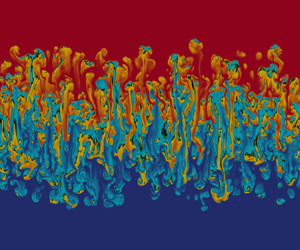
where $L$ is the mixing zone extent, $\mathcal {A} = (\rho _1-\rho _2)/(\rho _1+\rho _2)$ the Atwood number with $\rho _1$ and $\rho _2$ the densities of the heavy and light fluids, respectively, $g$ the magnitude of the local acceleration, and $\alpha$ the bubbles growth rate, whose determination is of primary importance (Dimonte et al. 2004). The present RTI configuration is presented in figure 1, with a developing mixing layer of extent $L(t)$. Note that (1.1) is valid within the Boussinesq approximation since it implies symmetry between the light and heavy fluids.

Figure 1. Vertical slice in the $(x_1, x_3)$ plane of the density field from DNS R4B0G10b of table 1 at $t=7$. The colourbar is the same as in figure 2, with the density and concentration related by $\rho =\rho _0[1 + 2\mathcal {A}(C-1/2)]$, where $\rho _0=(\rho _1+\rho _2)/2$ is the reference density.

Putting aside considerations regarding the values of $\alpha$ between DNS and experiments, we rather ask ourselves what we can learn about mixing by investigating the growth rate. Part of the answer has been provided by Gréa (2013) in the framework of miscible fluids. It was shown that the bubbles growth rate $\alpha$ is related to the mixing parameter ($\varTheta$, defined later in (4.1)), which quantifies how well the two fluids are mixed, and to the scalar anisotropy parameter ($\sin ^2 \gamma$, defined later in (4.2)), which reflects the stretching of the structures. Basically, the growth rate decreases when mixing at a molecular level increases; this can be understood with physical arguments. Considering bubbles of fluids forming at the interface and growing, they mix as they rise and fall due to small-scale shear instabilities; hence, the effective density contrast between the rising bubbles and the surrounding heavy fluid is smaller than $(\rho _1-\rho _2)$. Therefore, the magnitude of the production term decreases and the growth of the mixing zone slows down (Llor & Bailly 2003). If the falling and rising structures were to remain composed of pure fluids (no mixing), the density contrast would remain close to $(\rho _1-\rho _2)$ and the growth of $L$ would be faster. This phenomenology will be important in the interpretation of the results later on.

Since the self-similar state of the Rayleigh–Taylor instability is characterized by the growth rate of the mixing zone, it is fair to look for ways to modify it. The review by Dimonte et al. (2004) showed indeed that initial conditions (at large or small scales) affect the growth rate; this was more recently investigated by Kord & Capecelatro (2019), where optimal surfaces of perturbations were found to increase $\alpha$. The question of initial conditions was further addressed in the context of gravity reversals (Aslangil, Banerjee & Lawrie 2016), a framework in which the RTI can be suppressed (Boffetta, Magnani & Musacchio 2019). Adding a mean body rotation was also found to strongly impact the RTI and to decrease significantly the growth rate (Baldwin, Scase & Hill 2015; Boffetta, Mazzino & Musacchio 2016; Scase, Baldwin & Hill 2017). When considering porous media, the self-similar state does not follow (1.1) any longer (Boffetta, Borgnino & Musacchio 2020).

For conducting fluids, the outcomes are numerous. In experiments, ferrofluids were used to better control the onset of the RTI (Baldwin et al. 2015). From the linear stability analysis point of view, it is known since the work by Chandrasekhar (1961) that for a mean magnetic field applied parallel to the interface, perturbations below some critical wavelength along the mean field direction are damped (undular modes), whereas perturbation normal to it, still in the plane of the interface (interchange modes), are unstable like in the hydrodynamic case. The exponential growth rate $\sigma$ of the perturbations, for a flat interface between inviscid fluids for ideal MHD, is then given by

(1.2)\begin{equation} \sigma = \sqrt{\mathcal{A}gk_\perp - ({\boldsymbol k_\perp} \boldsymbol{\cdot} {\boldsymbol B_0})^2},\end{equation}

with $\boldsymbol k_\perp$ the horizontal wavevector of modulus $k_\perp$ and $B_0 = |{\boldsymbol B_0}|$ the mean magnetic field intensity scaled as the Alfvén velocity. More sophisticated configurations with mean magnetic fields parallel to the interface were also addressed in the past years to better interpret observations made in the astrophysical context, like the stability of a slab of heavy fluid (Terradas, Oliver & Ballester 2012), the effects of sheared magnetic fields (Ruderman, Terradas & Ballester 2014), compressibility, combination with Kelvin–Helmholtz instability and smooth density profiles (Hillier 2020).

When it comes to the linear stability of perturbations for a mean magnetic field perpendicular to the interface, the situation is different. As shown by Chandrasekhar (1961) and later by Jun, Norman & Stone (1995), there is no critical wavelength: all modes are unstable, with a growth rate decreased compared to the hydrodynamic case,

(1.3)\begin{equation} \sigma^3 + \sigma^2 k_\perp B_0 (\sqrt{r_1}+\sqrt{r_2}) + \sigma (k_\perp^2 B_0^2 - \mathcal{A}g k_\perp) = \frac{2 \mathcal{A} g k_\perp^2 B_0}{\sqrt{r_1}+\sqrt{r_2}}, \end{equation}

with $r_1=\rho _1/\rho _0$ and $r_2=\rho _2/\rho _0$. At large wavenumbers $k_\perp \gg 1$, the growth rate tends towards a constant value, namely $\sigma _\infty = g(\sqrt {r_1}-\sqrt {r_2})/B_0$. Later, Vickers, Ballai & Erdélyi (2020) considered an oblique $B_0$, with components normal and parallel to the interface, and showed that all modes become unstable.

Leaving the linear stability, the fully turbulent state of the magnetic Rayleigh–Taylor instability (MRTI) has been much less studied and almost exclusively, to our knowledge, with a mean magnetic field parallel to the interface. In early two-dimensional (2-D) DNS, with either a parallel or perpendicular mean magnetic field, Jun et al. (1995) observed elongated structures at onset, with a strong induced perpendicular magnetic energy. Depending on the magnitude of $B_0$, either an enhanced or damped growth of the mixing zone was observed. Later, three-dimensional (3-D) simulations of the MRTI were conducted by Stone & Gardiner (2007b) with a tangential magnetic field. They observed an increase of the mixing layer growth rate consistently with a reduction of small-scale mixing by magnetic tension. A magnetic shear at the interface was found to produce more isolated fingers, reminiscent of young supernova remnants (Stone & Gardiner 2007a). Again for the parallel magnetic field case, Carlyle & Hillier (2017) conducted 3-D DNS with the extent of the domain in the horizontal direction perpendicular to ${\boldsymbol B_0}$ much smaller than in the direction along ${\boldsymbol B_0}$: this lateral confinement may have contributed to the decrease of the bubbles growth rate with increasing magnetic field intensity. Conjointly, the spikes growth rate was observed to increase, thus strengthening the system asymmetry.

Hence, the fate of the MRTI in the turbulent regime for conducting fluids is not clear and we wish to bring some more understanding. What can we say about the growth rate of the turbulent mixing layer between two miscible conducting fluids, whose dynamics is described by the MHD equations (Biskamp 2003)?

The MRTI can play an important role in a variety of fields. In inertial confinement fusion (ICF), hydrodynamic instabilities may cool down the capsule hot-spot (Remington et al. 2019): in such devices, strong magnetic fluxes might be generated through the Biermann battery effect and hence should be accounted for when designing capsules (Walsh & Clark 2021).

The MRTI is also thought to be at the origin of elongated structures in several astrophysical systems, like expanding young supernova remnants (Jun et al. 1995; Jun & Norman 1996) with the Crab nebula as the most famous example, at the interface between the pulsar wind nebulae and the supernova shell (Cox, Gull & Green 1991; Porth, Komissarov & Keppens 2014), and in emerging magnetic fluxes (Isobe et al. 2005). The MRTI is also present in quiescent solar prominences (also called solar filaments), which are robust objects that may last for weeks in the solar corona and which are composed of cool dense plasma of the chromosphere, supported against gravity by magnetic tension (Ryutova et al. 2010; Hillier 2018). Often, vertical structures (called plumes or threads) are observed, either rising from the bubble/cavity interface below the prominence or falling from the cool dense plasma that constitutes the arch filament. There is a general consensus that the MRTI is responsible for the plumes' vertical dynamics within the prominences that simulations are able to reproduce qualitatively (Keppens, Xia & Porth 2015; Jenkins & Keppens 2022). The determination of the magnetic field orientation in solar prominences is complex: nevertheless, measurements indicate that it is mainly aligned with the line of sight, or in other words, tangential to the solar limb (Leroy 1989). Still, normal components cannot be ruled out (Vickers et al. 2020). Moreover, in recent simulations aimed at reproducing the prominences dynamics (Keppens et al. 2015; Jenkins & Keppens 2022), the initial magnetic fields are often inhomogeneous and possibly with normal components.

From the thorough analysis of images taken by the Solar Optical Telescope aboard Hinode, numerous authors have measured and estimated characteristic features of quiescent solar prominences and tested them against various models. For instance, from the descending speed of bright knots (${\sim }16\ {\rm km}{\cdot } {\rm s}^{-1}$), the magnetic field strength was found to be of the order of 5 to 7 G (Chae 2010). Also, using the MRTI framework, Ryutova et al. (2010) inferred the ambient magnetic field intensity from the measure of the exponential growth rate of plumes using the linear stability (1.2).

However, one may ask to what extent this method may be adequate to describe the growth of elongated structures around fully turbulent astrophysical objects. Basically, as a rule of thumb, for a structure of wavelength $\lambda =2{\rm \pi} /k_\perp$, if its height exceeds a few percent of $\lambda$, this means that nonlinear mechanisms are already at play (Sharp 1984). Hence, there is a need to investigate in more detail the fully turbulent state of the MRTI. Additionally, the brief review presented earlier revealed that it remains partially unclear. To shed some light on the asymptotic state of the MRTI, we simplify the problem by considering the incompressible limit within the Boussinesq approximation, as suggested by Jun et al. (1995) some time ago. Since the parallel $B_0$ configuration creates some additional complexities due to non-axisymmetric statistics, we rather consider a uniform vertical $B_0$ perpendicular to the interface, where statistical axisymmetry is preserved, so that classical RTI models can a priori be extended to MHD. Both frameworks share some similarities because they yield dominant perpendicular induced magnetic energy. This is relevant for young supernova remnants (Jun & Norman 1996; Inoue et al. 2013), for interactive outflows of a close-in planet and its host star (Matsakos, Uribe & Königl 2015), and possibly also for quiescent (Vickers et al. 2020) and active solar prominences where the perpendicular component can be much stronger (Leroy 1989).

In a previous work (Briard, Gréa & Nguyen 2022), we have derived an analytical relation between the growth rate of the mixing zone in the MRTI with a perpendicular $B_0$, the ambient magnetic field intensity, mixing and anisotropy. This prediction for the growth rate, which relies on the turbulent properties of the flow, was successfully compared with high-resolution DNS. Moreover, in a companion paper (Gréa & Briard 2023), we have determined the terminal velocity of rising bubbles in the potential regime of rapid growth, thus extended the theory of Goncharov (2002) for the MRTI with an inclined $B_0$.

In the present paper, we pursue this study and go into the details of the numerous MRTI simulations conducted. After presenting the equations and the numerical set-up in § 2, we propose some physical interpretation for the delayed transition to turbulence in the presence of a mean magnetic field in § 3. The main effects of varying the intensity of $B_0$ upon the dynamics are exposed and quantified in § 4, where global quantities are examined, along with horizontally averaged vertical profiles, and the energy budget is addressed. Section 5 gathers the details of our finest DNS with $4096^3$ points for the hydrodynamic reference case, with in particular spectral scale-by-scale analysis. A similar investigation is performed in the following § 6 for our finest DNS of the MRTI: the main findings of Briard et al. (2022) are recalled, in particular, the prediction of the growth rate of the mixing layer in the MRTI, with additional details about the derivation and further comparisons with DNS. The conclusions are grouped in the final section. Several appendices are also proposed for the sake of completeness, with the equations of the main correlations in both physical and spectral spaces in Appendix A, considerations about numerical details in Appendix B, details regarding stability analysis in Appendix C, and finally additional discussions in Appendix D about the effects of Reynolds number and viscosity, sorted concentration field and the transport of magnetic energy.

2. Main equations and numerical set-up

2.1. Evolution equations

In the following, we consider two fluids initially separated by a horizontal perturbed interface, with the heavier fluid on top of the lighter one in a downward gravity field $\boldsymbol g = - g {\boldsymbol n_3}$, with $\boldsymbol n_3$ the vertical unit vector. The incompressible Navier–Stokes equations within the Boussinesq and MHD approximations read

(2.1a)$$\begin{gather} \frac{\partial \boldsymbol U}{\partial t} + (\boldsymbol U \boldsymbol{\cdot} \boldsymbol \nabla) \boldsymbol U ={-} \boldsymbol \nabla P - 2 \mathcal{A} g C {\boldsymbol n_3} + (\boldsymbol \nabla \times \boldsymbol B ) \times \boldsymbol B + \nu \nabla^2 \boldsymbol U, \end{gather}$$

(2.1b)$$\begin{gather}\frac{\partial \boldsymbol B}{\partial t} + (\boldsymbol U \boldsymbol{\cdot} \boldsymbol \nabla) \boldsymbol B = (\boldsymbol B \boldsymbol{\cdot} \boldsymbol \nabla) \boldsymbol U + \eta \nabla^2 \boldsymbol B, \end{gather}$$

(2.1c)$$\begin{gather}\frac{\partial C}{\partial t} + (\boldsymbol U \boldsymbol{\cdot} \boldsymbol \nabla) C = \kappa \nabla^2 C, \end{gather}$$

(2.1d)$$\begin{gather}\boldsymbol \nabla \boldsymbol{\cdot} \boldsymbol U = 0, \end{gather}$$

(2.1e)$$\begin{gather}\boldsymbol \nabla \boldsymbol{\cdot} \boldsymbol B = 0, \end{gather}$$

where $\boldsymbol U$ is the total velocity field, $\boldsymbol B$ the magnetic field scaled as a velocity ($\boldsymbol B = {\boldsymbol H}/\sqrt {\rho _0 \mu _0}$, where ${\boldsymbol H}$ is the true magnetic field, $\mu _0$ the vacuum magnetic permeability and $\rho _0=(\rho _1 + \rho _2)/2$ the reference density) and $C$ the concentration of the heavy fluid. Additionally, $P$ is the reduced pressure, and $\nu$, $\eta$ and $\kappa$ are the kinematic viscosity, magnetic diffusivity and molecular diffusivity, respectively.

For the Rayleigh–Taylor configuration, we assume homogeneity of the statistics in horizontal planes, so that we can decompose any field $A$ into its horizontal average $\langle A \rangle$ and its fluctuating part $a=A- \langle A \rangle$. The volume average is denoted by $\bar {\star }$ and is obtained by an additional integration over the vertical direction, weighted by the mixing zone length $L$ defined in (2.4). For example, the volume average of the correlation between two fluctuating fields $a_1$ and $a_2$ read

(2.2)\begin{equation} \overline{a_1 a_2}(t) = \frac{1}{L} \int \langle a_1 a_2 \rangle (x_3, t) \, \mathrm{d}\kern 0.06em x_3.\end{equation}

Note that fluctuations decrease quickly outside the mixing layer, so that integration along the whole vertical direction amounts to averaging upon the mixing zone width for second-order correlations.

In the particular case of the magnetic Rayleigh–Taylor instability, we consider the additional presence of a vertical uniform mean magnetic field, so that the total magnetic field reads $\boldsymbol B = B_0 {\boldsymbol n_3} + \boldsymbol b$ (with $\boldsymbol B$ normalized as a velocity, $B_0$ can be interpreted as the mean Alfvén velocity). It is also convenient to express the Lorentz force $(\boldsymbol \nabla \times \boldsymbol B ) \times \boldsymbol B = - \boldsymbol \nabla (B^2/2) + (\boldsymbol B \boldsymbol {\cdot } \boldsymbol \nabla ) \boldsymbol B$ as the sum of magnetic pressure, which is included in the total pressure, and magnetic tension. In addition, note that in this configuration, there are no induced mean magnetic fields, so that $B_0$ remains constant, see Appendix A.1. After some algebra, the equations for the fluctuations read, in the absence of mean velocity and magnetic fields,

(2.3a)$$\begin{gather} \frac{\partial u_i}{\partial t} + \frac{\partial u_j u_i}{\partial x_j} ={-} \frac{\partial \varPi}{\partial x_i} - 2 \mathcal{A} g c \delta_{i3} + \frac{\partial b_i b_j}{\partial x_j} + B_0 \frac{\partial b_i}{\partial x_3} + \frac{\partial}{\partial x_3} \langle u_i u_3 - b_i b_3 \rangle + \nu \nabla^2 u_i, \end{gather}$$

(2.3b)$$\begin{gather}\frac{\partial b_i}{\partial t} + \frac{\partial u_j b_i}{\partial x_j} = \frac{\partial b_j u_i}{\partial x_j} + B_0 \frac{\partial u_i}{\partial x_3} + \frac{\partial}{\partial x_3} \langle u_3 b_i - u_i b_3 \rangle + \eta \nabla^2 b_i, \end{gather}$$

(2.3c)$$\begin{gather}\frac{\partial c}{\partial t} + \frac{\partial u_j c}{\partial x_j} ={-} u_3 \frac{\partial }{\partial x_3} \langle C \rangle + \frac{\partial}{\partial x_3} \langle u_3 c \rangle + \kappa \nabla^2 c. \end{gather}$$

In these equations, summation upon repeated indices is used. Both mean velocity and magnetic fields are negligible in this configuration. Here, $\varPi = p + (b_j b_j - \langle b_j b_j \rangle )/2$ is the generalized pressure, with $p=P-\langle P \rangle$ the fluctuating reduced pressure. Equations for the two-point correlations are given in Appendix A.2. In addition to the usual nonlinear and dissipative terms, the above set of (2.3a)–(2.3c) contains several linear terms: the production of velocity and magnetic fluctuations through the mean magnetic field, namely $B_0 \partial _3 \boldsymbol u$ and $B_0 \partial _3 \boldsymbol b$, and also the production of scalar fluctuations through the enlargement of the turbulent mixing zone via $-u_3 \partial _3 \langle C \rangle$. Note that the inverse mean concentration gradient can be used to evaluate the mixing zone width, with $1/L \simeq \partial _3 \langle C \rangle$. In practice, here we use the integral definition (Andrews & Spalding 1990)

(2.4)\begin{equation} L(t) = 6 \int \langle C \rangle ( 1 - \langle C \rangle ) \,\mathrm{d}\kern 0.06em x_3.\end{equation}

Equations (2.3) indicate that for an initially perturbed interface between the heavy and light fluids, vertical velocity fluctuations $u_3$ are created through the buoyancy term $- 2 \mathcal {A} g c$, which then produces additional concentration fluctuations through $-u_3 \partial _3 \langle C \rangle$ and generates magnetic fluctuations as well through the term $-B_0 \partial _3 u_i$. In the following, we will investigate how the induced magnetic field can alter the development of the turbulent mixing zone.

2.2. Numerical set-up

We have performed direct numerical simulations (DNS) of the incompressible Navier–Stokes equations (2.1a)–(2.1e) under the Boussinesq and MHD approximations, with the pseudo-spectral code STRATOSPEC (Briard, Gostiaux & Gréa 2020). The domain is a triply periodic box of dimensions $(L_{x_1}, L_{x_2}, L_{x_3})$, with always $L_{x_1} = L_{x_2} = 2 {\rm \pi}$.

The present simulations have resolution from $1024^2 \times 2048$ points to $4096^3$ points, and are performed with a pencil decomposition, using from 2048 up to 65 536 cores. A classical spectral Fourier collocation method is used with two-third rule dealiasing, so that the maximum wavenumber is $k_{max}=N_1/3$, with $N_1$ the number of points in the $x_1$ direction. The P3DFFT algorithm was implemented to perform massively parallel fast Fourier transforms (Pekurovsky 2012). The time increment is determined using a third-order low-storage strong-stability-preserving Runge–Kutta scheme, with implicit treatment of diffusive terms.

The initial conditions are detailed in Appendix B.1. The main features are that the velocity and fluctuating magnetic fields are initially zero. The initial perturbation of the interface between the heavy and light fluids is driven by a three-dimensional concentration variance spectrum $E_{cc}$, whose peak wavenumber $k_p$ and initial variance $\overline {c^2}(t=0)$ are given in table 1.

Table 1. Parameters of the DNS: Number of points $N$, Vertical extent $L_{x_3}$ (with always $L_{x_1}=L_{x_2}=2{\rm \pi}$), Buoyancy strength $\mathcal {A}g$, with $\mathcal {A}=0.05$ the Atwood number and $g$ the acceleration, Mean vertical magnetic field intensity $B_0$ (scaled as a Alfvén velocity), Kinematic viscosity $\nu = \kappa$, Magnetic Prandtl number $P_M = \nu /\eta$, and Peak wavenumber $k_p$ of the initial concentration spectrum (all runs have initially $\overline {c^2} (t=0) = 0.022$ and $\varTheta (t=0)=0.867$), Self-similar value of the magnetic to kinetic energy ratio $R_{ss}$, Ratio of the maximum and Kolmogorov wavenumbers $k_{max}/k_\eta$ at the final time $t_{end}$ of the simulation.

The parameters of the different DNS are gathered in table 1. The simulations starting with label R1 refer to resolution $1024^2 \times 2048$, with a computational domain vertically elongated, with $L_{x_1}=L_{x_2} = L_{x_3}/2=2{\rm \pi}$. Some of these simulations were duplicated in the cubic domain $L_{x_1}=L_{x_2} = L_{x_3}=2{\rm \pi}$, with resolution $1024^3$, but are not presented in table 1 for the sake of conciseness. They only serve to estimate vertical confinement effects, to address the spatial resolution of the simulations in Appendix B.2 and for illustration purposes, like in figure 2. Hence, only the R1 simulations in the elongated domain are presented in table 1 since they permit to reach a fully developed turbulent asymptotic state.

Figure 2. Concentration field $C$ from the simulations R1B0G10, R1B020G10 and R1B050G10 ($1024^3$) for different mean magnetic field intensities – from left to right, $B_0=0$, $B_0=0.20$ and $B_0=0.50$ – at four different instants – from top to bottom, $t=0$, $t=2$, $t=5$ and $t=8$. The colourmap is chosen so that the pure fluids ($C=0$ and $C=1$) are transparent, with a sharp colour gradient around $C=1/2$.

Simulations R2 with resolution $2048^3$ and cubic domain $(2{\rm \pi} )^3$ are used to address the spatial resolution in Appendix B.2, along with the effects of changing either the peak wavenumber of the initial condition or the diffusion coefficients in Appendix D. The only simulation with resolution $2048^2 \times 4096$ serves to reach a more turbulent self-similar state of the MRTI. Finally, simulations R4 have the finest resolution with $4096^3$ points and are used to address spectral scalings and scale-by-scale energy budget.

The subsequent letters in the labels are B for the mean magnetic field intensity $B_0$, and G for the value of the gravitational acceleration $g$ (note that $\mathcal {A}$ is not modified in this study). For some cases, an additional letter a or b is used to discriminate between different diffusion coefficients. Note that the peak wavenumber $k_p$ is different for the R1, R2 and R4 simulations.

3. Phenomenology of the MRTI

3.1. Observations

Before performing a thorough analysis of the flow generated by the magnetic Rayleigh–Taylor instability, we first show in figure 2 the 3-D concentration field $C$, extracted from the R1 simulations at different instants, with varying mean magnetic field intensity $B_0$. The colourmap is chosen so that the pure fluids ($C=0$ and $C=1$) are transparent, with a sharp colour gradient around $C=1/2$. From left to right, $B_0$ is increased, and from top to bottom, time goes by. A supplementary movie is available at https://doi.org/10.1017/jfm.2023.1053 of the developing instability.

Starting from the same initial condition (the same perturbed interface), it is clear that at $t=2$, the onset of the Rayleigh–Taylor instability is already greatly modified by the presence of the mean magnetic field. In the purely hydrodynamic case, typical bubbles of different sizes appear. For $B_0=0.2$, the initial perturbations are vertically stretched. For the even stronger Alfvén velocity $B_0=0.5$, the instability is delayed, with the growth rate of the perturbations damped by the mean magnetic field (Chandrasekhar 1961).

Later on, at $t=5$, turbulent structures are visible for the non-magnetic case, with multiple colours on the 3-D concentration field, illustrating mixing at different levels. For $B_0=0.2$, bubbles have also formed at the edges of the developing elongated structures, which shows some resemblance with the previous case $B_0=0$ at $t=2$, but with a wider mixing layer. For $B_0=0.5$, the initial perturbations have only been stretched, revealing smooth elongated fingers, with apparently no mixing.

At $t=8$, the turbulent mixing zone has grown in size for both $B_0=0$ and $B_0=0.2$, but interestingly, it is wider for the latter case. Despite the initial inhibition of the shear instabilities, turbulent mixing has been enhanced afterwards. Finally, for $B_0=0.5$, the smooth elongated fingers are still being stretched, with bubbles eventually forming at their edges, with no mixing between ascending and descending structures.

The phenomenology depicted here is interesting and reveals several noteworthy features. Compared with the purely hydrodynamic case, the mean vertical magnetic field initially delays the instability, but later enhances turbulent mixing, as seen with $B_0=0$ and $B_0=0.2$ at $t=5$. This was first evidenced in the early 2-D simulations of Jun et al. (1995) and is confirmed here in 3-D high-resolution simulations. In the regime where magnetic effects dominate, structures are elongated and smooth fingers appear, rather than turbulent bubbles; small-scale shear instabilities are inhibited and there is no turbulent mixing, yielding a rapid growth of the mixing zone $L$.

In the two following parts, in a simplified and idealized framework, a criterion for the fingers to be destabilized is determined, and some explanations are proposed for the appearance of elongated structures.

3.2. Shear instability between ascending and descending structures

In this part, we perform a simplified linear stability analysis to provide a criterion for which the vertically elongated fingers observed previously are destabilized by small-scale shear instabilities.

We consider a 2-D inviscid framework and choose to model the two elongated fingers by two semi-infinite planes, separated at some initial time $t_0$ by a flat interface. The falling pure heavy fluid of density $\rho _1$ and the ascending light one of density $\rho _2$, within the Boussinesq approximation, have opposite constant velocities $\pm V$. The mean magnetic field $B_0$ is oriented upward and the gravitational acceleration $g$ downward. The configuration is sketched in figure 3 with, for this section only, $x_1=0$ indicating the interface position ‘at rest’ between ascending and descending structures. It is worth noting that the framework just described corresponds in fact, after a $90^\circ$ clockwise rotation, to an almost classical Kelvin–Helmholtz configuration (Chandrasekhar 1961), with a mean magnetic field parallel to the interface, but in which the gravity would be horizontal, opposite to $B_0$.

Figure 3. Sketch of the 2-D configuration for the present linear stability analysis.

The details of the linear stability analysis are gathered in Appendix C for the sake of conciseness and only the result is given here: the interface between the ascending and descending fluids is unstable if

(3.1)\begin{equation} V^2 > B_0^2,\end{equation}

meaning that the typical velocity of the fingers should exceed the Alfvén velocity imposed by the vertical mean magnetic field. This simple criterion, also proposed by Jun et al. (1995), is compared with DNS in § 4. It provides only a lower bound for transition to turbulence to occur. Indeed, the real elongated structures are not semi-infinite planes, have finite thickness and are separated by a diffuse interface. These features participate in the reduction of the instability growth rate (Miura & Pritchett 1982). Hence we expect transition to turbulence to occur for velocities larger than $B_0$.

Finally, note that the stability of a shear flow with an aligned mean magnetic field was addressed by Hughes & Tobias (2001) for arbitrary background velocity and magnetic fields. In the simple case of a uniform $B_0$ and constant piecewise velocity field, it reduces to (3.1).

3.3. Homogeneous turbulence approach

In the previous section, the destabilization of the elongated fingers due to the shear between ascending and descending structures has been investigated. When these smooth fingers break and the flow becomes turbulent, it is expected that due to magnetic tension, structures remain aligned with magnetic field lines, namely stretched in the vertical direction. To analyse this phenomenology in more detail, we use the spectral formalism, which is a corner stone of the developments and predictions made later in § 6.4. For simplicity, we assume that turbulent fluctuations within the core of the mixing layer are homogeneous in the three directions and that they ‘see’ only the mean concentration gradient $\partial _3 \langle C \rangle =1/L$: in the non-magnetic case, this framework is known as unstably stratified homogeneous turbulence (Griffond, Gréa & Soulard 2014; Soulard, Griffond & Gréa 2014; Burlot et al. 2015; Griffond, Gréa & Soulard 2015; Gréa et al. 2016; Briard, Iyer & Gomez 2017). Then, we discard the nonlinearities along with diffusion terms, which do not act at the large scales considered, keeping only interactions with the mean flow, which is reminiscent of the rapid distortion theory (Hunt & Carruthers 1990). The resulting equations for the spectral vertical fluctuations are

(3.2a)$$\begin{gather} \frac{\partial \hat{u}_3}{\partial t} ={-} 2 \mathcal{A}g \hat{c}(\boldsymbol k) P_{33}(\boldsymbol k) + \mathrm{i} k_3 B_0 \hat{b}_3(\boldsymbol k), \end{gather}$$

(3.2b)$$\begin{gather}\frac{\partial \hat{b}_3}{\partial t} = \mathrm{i} k_3 B_0 \hat{u}_3(\boldsymbol k), \end{gather}$$

(3.2c)$$\begin{gather}\frac{\partial \hat{c}}{\partial t} ={-} \frac{1}{L} \hat{u}_3(\boldsymbol k), \end{gather}$$

where $\hat {{\cdot }}$ represents the Fourier transform and $P_{ij}=\delta _{ij}-k_i k_j/k^2$ the projector onto the plane perpendicular to the wavevector $\boldsymbol k$. The complete spectral equations for the fluctuating fields are given in Appendix A.3. Combining the previous equations readily gives

(3.3)\begin{equation} \frac{\partial^2 \hat{u}_3}{\partial t^2} + ( k^2 B_0^2 \cos^2 \theta - N^2 \sin^2 \theta ) \hat{u}_3 = 0, \end{equation}

where $\theta$ is the angle between $\boldsymbol k$ and the vertical ${\boldsymbol n}_3$, and $N=\sqrt {2 \mathcal {A}g/L}$ the buoyancy frequency (similar equations for $\hat {c}$ and $\hat {b}_3$ can be obtained). In the absence of a magnetic field, it is recovered that the modes with wavevector $\boldsymbol k$ pertaining to the equatorial plane ($\theta ={\rm \pi} /2$) are the most amplified (Soulard et al. 2014). The striking difference in the magnetic case is that for all other orientations, $\theta \neq {\rm \pi}/2$, the modes are damped by the mean magnetic field, which forces the structures to remain aligned with the field lines.

3.4. Conclusions on the phenomenology

Using simple models, we have explained two features of the phenomenology observed in figure 2. First, the vertical mean magnetic field inhibits mixing by preventing small-scale shear instabilities between ascending and descending structures. In this early regime, the mixing layer grows faster than in the hydrodynamic case. These structures eventually break when the turbulent vertical velocity becomes strong enough: they are vertically stretched because the mean magnetic field damps modes with wavevectors not in the plane parallel to the initial interface. Therefore, at transition to turbulence, the mixing layer might be larger in the presence of a vertical mean magnetic field than in the hydrodynamic case.

So far, we have evidenced that the induced and imposed magnetic fields strongly impact the onset of the Rayleigh–Taylor instability and transition to turbulence: this will be better quantified in the next section. Once the flow is fully turbulent, despite a persistent strong vertical anisotropy, a classical phenomenology seems to be recovered. Whether magnetic energy overcomes kinetic energy or not is investigated later in § 4, and in § 6 for the self-similar regime of the MRTI.

4. Quantitative description of the MRTI dynamics

In this section, an overview of the different results with the R1 simulations is presented to understand the effects of varying the intensity of the mean vertical magnetic field $B_0$ on the development of the MRTI. One-point statistics are investigated, along with more refined features, such as vertical profiles of horizontally averaged quantities. Irreversible mixing, anisotropy, transition to turbulence and energy budgets are addressed. In §§ 5 and 6, the emphasis is put on the finest simulations with $4096^3$ points, with first the hydrodynamic case as a reference, and then the magnetic configuration, with detailed spectral scalings and scale-by-scale information.

4.1. Overall dynamics, anisotropy and mixing

In this part, we focus on one-point statistics, which provide quantitative information about the dynamics, transition to turbulence and mixing. Additional details are given in Appendix D, notably regarding the Reynolds number, which can be defined in multiple ways.

The criterion (3.1), derived from the previous inviscid linear analysis, is now compared with DNS: we choose $V = (\overline {u_3^2})^{1/2}$ for the typical velocity of the ascending and descending fingers. It is revealed in figure 4(a) that for $V>B_0$, there is indeed a change of regime that occurs later for larger $B_0$. Elongated smooth fingers are destabilized by shear instabilities, mixing occurs, causing a net reduction of the vertical velocity: this is transition to turbulence. Afterwards, the growth rate of the vertical velocity is decreased compared to the initial phase. For the case $B_0=0.5$, $V$ hardly reaches the Alfvén velocity, consistent with the observations of figure 2. In contrast, for the weak field $B_0=0.1$, the initial growth is quite comparable to the RTI case so that $V$ reaches large values before destabilization. As expected from the discussion at the end of § 3.2, transition to turbulence happens after the criterion (3.1) is fulfilled. The ratio $M_A=V/B_0$ can be interpreted as an Alfvén Mach number and shows that the turbulent state of the MRTI corresponds to $M_A>1$.

Figure 4. Effects of the mean magnetic field intensity $B_0$ in the R1 simulations. (a) Normalized vertical velocity with the Alfvén velocity $\sqrt {\overline {u_3^2}}/B_0$, see criterion (3.1). (b) Mixing zone size $L$ (2.4).

We pursue the analysis by investigating the mixing layer growth in figure 4(b). As observed in figure 2, the presence of a vertical mean magnetic field slows down the onset of the instability: a stronger $B_0$ results in a slower initial growth. This is qualitatively in agreement with the theory since the smallest wavelengths have their growth rate damped (Chandrasekhar 1961). Later on, with the magnetic field acting as a tension that inhibits small-scale shear instabilities, the elongated fingers grow more rapidly than the merging bubbles. With larger $B_0$, transition to turbulence is delayed and the width of the mixing layer can be significantly larger than in the hydrodynamic case. Then, turbulent mixing occurs and the growth of $L(t)$ is slowed down. Dimensional analysis indicates that two regimes are possible for the mixing layer: either $L \sim B_0 t$ or $L \sim \mathcal {A}g t^2$. Consistent with the previous discussion, the former corresponds to the transient regime of rapid growth with $M_A<1$: structures are rapidly stretched without mixing and grow at a constant velocity (Gréa & Briard 2023), whereas the latter, which is the standard self-similar regime of the RTI (Youngs 1994), is recovered after transition to turbulence and corresponds to $M_A>1$. The turbulent mixing layer growth rate, modified by the presence of induced magnetic energy, is thoroughly analysed later in § 6.

It has been observed in figure 2 that a larger $B_0$ means that mixing occurs later, since the mean magnetic field inhibits shear instabilities at small scales. To quantify mixing, we use the mixing parameter $\varTheta$ (Youngs 1994) defined as

(4.1)\begin{equation} \varTheta = \frac{\displaystyle \int \langle C (1-C) \rangle \,\mathrm{d}\kern 0.06em x_3}{\displaystyle \int \langle C \rangle \langle (1-C) \rangle \mathrm{d}\kern 0.06em x_3} = 1- 6 \overline{c^2}, \end{equation}

and presented in figure 5(a). Indeed, during the initial phase of elongated fingers, the mixing parameter is small $\varTheta \simeq 0.4$. When the vertical turbulent velocity exceeds the Alfvén velocity and transition to turbulence occurs, the mixing parameter increases, a phenomenology consistent with the observations of Cook, Cabot & Miller (2004). The final values of the mixing parameter for $B_0 \leq 0.2$ are quite close to the non-magnetic case, with $0.76 \leq \varTheta \leq 0.80$, which is a classical range (Gréa 2013). Interestingly, for $B_0=0.3$, the mixing parameter is larger than in the non-magnetic case, with $\varTheta \simeq 0.83$: despite the long transient regime, mixing is eventually more efficient. This can be interpreted as follows: due to the vertical stretching of the structures, the surface available for mixing and mass exchanges at the time of transition to turbulence is greater.

Figure 5. Effects of the mean magnetic field intensity $B_0$ in the R1 simulations: (a) mixing parameter $\varTheta$ (4.1); (b) global anisotropy indicator $\sin ^2 \gamma$ (4.2).

The directional anisotropy of the concentration field can be analysed through the dimensionality parameter $\sin ^2 \gamma$, expressing the ratio between the amplitudes of the two first spherical harmonics, defined as

(4.2)\begin{equation} \sin^2 \gamma = \frac{\displaystyle \int \mathcal{E}_{cc}(\boldsymbol k) \sin^2 \theta \,\mathrm{d}V_k}{\displaystyle \int \mathcal{E}_{cc}(\boldsymbol k) \,\mathrm{d}V_k}, \end{equation}

where $\mathcal {E}_{cc}$ is the spectral concentration variance such that $L_{x_3} \int \mathcal {E}_{cc} \, \mathrm {d}V_k = L\overline {c^2}$, with $\mathrm {d}V_k$ the infinitesimal spherical volume in spectral space. This parameter takes the value 2/3 for an isotropic field, such that $2/3 \leq \sin ^2 \gamma \leq 1$ for vertically stretched structures and such that $0 \leq \sin ^2 \gamma \leq 2/3$ for flat ones.

This anisotropy indicator is presented in figure 5(b) for various $B_0$. When there is an effective transition to turbulence, i.e. when $\varTheta$ increases in figure 5(a), $\sin ^2 \gamma$ is significantly reduced due to the partial return to isotropy of the smallest scales of the flow. In the asymptotic regime – which is not reached for $B=0.5$ – a stronger $B_0$ results in a larger $\sin ^2 \gamma$, which indeed corresponds to vertically stretched structures. This shows that there is a persistent effect of the mean magnetic field on the Rayleigh–Taylor instability, even after transition to turbulence.

Another way to observe the delayed transition to turbulent mixing in the MRTI is to analyse the time evolution of the concentration probability density function $f(C)$. To make the visualization easier, we restrict our attention to the middle plane $x_3=0$ and investigate how the distribution $f(C)$ evolves with time for $B_0=0$ and $B_0=0.2$ in figures 6(a) and 6(b), respectively. Initially, due to the perturbed interface, there are mostly values around $C \simeq 1/2$. However, when the instability develops, pure heavy fluid falls down while light fluid goes up, showing the strong values of $f(C)$ for $C=0$ and $C=1$ (the maximum value is set at $3$ for readability). Then, around $2 \leq t \leq 3$, turbulent mixing starts for $B_0=0$ and a wide range of intermediate $C$-values appears. For the magnetic case, it takes much longer for turbulent mixing to occur.

Figure 6. Probability density function $f(C)$ of the concentration field at the plane $x_3=0$ as a function of time: (a) for $B_0=0$ (R1B0G10); (b) for $B_0=0.2$ (R1B020G10).

In figures 7(a) and 7(b), the time evolution of the kinetic energy $\mathcal {K}_{uu}=\overline {u^2}/2$ and magnetic energy $\mathcal {K}_{bb}=\overline {b^2}/2$, normalized by $\dot {L}^2$, are presented. After a transient growth, both ratios strongly decrease: this corresponds to the regime of rapid increase of $L(t)$, associated with the stretching of vertical structures with no mixing. Then, after transition to turbulence, $\mathcal {K}_{uu}/\dot {L}^2$ and $\mathcal {K}_{bb}/\dot {L}^2$ tend towards constant values at late times, except for $B_0=0.5$ where the flow is still in a transient phase. As discussed before, since $L(t)$ grows like $t^2$ in the self-regime of the MRTI, and thus $\dot {L} \sim t$, this shows that both $\mathcal {K}_{uu}$ and $\mathcal {K}_{bb}$ grow also like $t^2$.

Figure 7. Effects of the mean magnetic field intensity $B_0$ in the R1 simulations: (a) normalized kinetic energy $\mathcal {K}_{uu}$; (b) normalized magnetic energy $\mathcal {K}_{bb}$.

Moreover, while the asymptotic value of $\mathcal {K}_{uu}/\dot {L}^2$ seems quite independent of the vertical mean magnetic field for $0.1 \leq B_0 \leq 0.3$, the level of induced turbulent magnetic energy increases. It will be shown later in § 6 that the ratio $\mathcal {K}_{bb}/\mathcal {K}_{uu}$ is of primary importance to determine the growth rate of the mixing layer in the self-similar state of the MRTI.

Now that the global dynamics has been described, and the effects of a mean magnetic field upon mixing and anisotropy exhibited, we quantify transition to turbulence in the MRTI by investigating the turbulent Reynolds number

(4.3)\begin{equation} Re_T = \frac{\mathcal{K}_{uu}^2}{\nu \varepsilon_{uu}},\end{equation}

where $\mathcal {K}_{uu} = \overline {u_i u_i}/2$ is the kinetic energy and $\varepsilon _{uu} = \nu \overline {\partial _j u_i \partial _j u_i}$ its dissipation rate. In figure 8(a), the transition to turbulence is evidenced in the magnetic configurations by a strong decrease of the Reynolds number, corresponding to an important dissipation of energy. This is correlated to the onset of small-scale shear instabilities that makes $\varTheta$ increase and $\sin ^2\gamma$ decrease. This is quite different from the hydrodynamic case, where $Re_T$ always increases. In addition, transition to turbulence happens for larger $Re_T$ when $B_0$ increases, basically around $Re_T \simeq 135$ for $B_0=0$, up to almost $Re_T = 10^3$ for $B_0=0.3$. Other definitions of the Reynolds number are discussed in Appendix D.2.

Figure 8. (a) Effects of the mean magnetic field intensity $B_0$ on the turbulent Reynolds number $Re_T$, defined in (4.3), for the R1 simulations. The cross indicates $t_{tr}$ for $B_0=0.3$. (b) Normalized transition time to turbulence $t_{tr}/T_{ref}$ as a function of the magnetic Froude number $F_M$ for all simulations of table 1. Colours refer to the diffusion coefficients: the green circle indicates the R1 simulation with $B_0=0.2$ and $P_M=1$ to be compared with the two simulations R1B020G10P1 and R1B020G10P2 with $P_M<1$.

We now turn our attention to the time $t_{tr}$ at which transition to turbulence occurs. Elongated structures are observed to break after the sudden decrease of $Re_T$ in figure 8(a). Therefore, we choose $t_{tr}$ as the time at which $Re_T$ reaches its minimum value, after the first maximum (for example, around $t\simeq 8$ for $B_0=0.3$). In addition, we define characteristic time, velocity and length scales as

(4.4a)$$\begin{gather} T_{ref} = \left( \frac{\nu}{(\mathcal{A}g)^2} \right)^{1/3} = \left( \frac{\eta}{(\mathcal{A}g)^2} \right)^{1/3} P_M^{1/3}, \end{gather}$$

(4.4b)$$\begin{gather}V_{ref} = ( \mathcal{A}g \eta )^{1/3} = ( \mathcal{A}g \nu )^{1/3} P_M^{{-}1/3}, \end{gather}$$

(4.4c)$$\begin{gather}L_{ref} = V_{ref} T_{ref} = \left( \frac{\eta^2}{\mathcal{A}g} \right)^{1/3} P_M^{1/3}, \end{gather}$$

where $P_M=\nu /\eta$ is the magnetic Prandtl number. These reference scales are chosen independent of the peak wavenumber $k_p$ at which perturbations are injected in the simulations, because we assume that $k_p$ is small enough for the asymptotic state to not depend significantly on it (the effect of $k_p$ is discussed later in figures 13a and 13b). Finally, we define global magnetic Froude and Reynolds numbers, which are related as

(4.5a,b)\begin{equation} F_M = \frac{B_0}{V_{ref}}, \quad R_M = \frac{L_{ref} B_0}{\eta} = P_M^{1/3} F_M.\end{equation}

In figure 8(b), when considering all simulations of table 1, the normalized transition time to turbulence $t_{tr}/T_{ref}$ shows two scalings as function of the magnetic Froude number $F_M$. For $F_M \leq 2$, $t_{tr}$ is relatively independent of $F_M$ because induced magnetic fields are not strong enough to modify significantly the dynamics. While for $F_M \geq 2$, $t_{tr}$ evolves linearly with $F_M$, and this illustrates once again the delayed transition to turbulence when increasing the mean magnetic field intensity. This scaling with $F_M$ is used later on to characterize the self-similar regime of the MRTI.

In figure 8(b), scaling with $R_M$ rather than $F_M$ would have slightly shifted towards the left the two simulations R1B020G10P1 and R1B020G10P2 with $P_M < 1$ (green squares). The black square circled in green indicates simulation R1B020G10 where $P_M=1$ for comparison.

4.2. Energy budget and irreversible mixing

In this section, the emphasis is put on the MRTI energy budget. In the Rayleigh–Taylor instability framework, the variation of potential energy with respect to its initial value corresponds to the energy injected into the system, and is defined as (Cook et al. 2004)

(4.6)\begin{equation} E_P=g \overline{x_3(\rho-\rho(0))} = \frac{g}{L} \int (\langle \rho \rangle - \rho(0) ) x_3 \, \mathrm{d}\kern 0.06em x_3 \simeq{-}\frac{\mathcal{A}g \rho_0 L}{12}. \end{equation}

The last equality stands for a linear mean density profile in the mixing zone, which is well verified in the present simulations. The total energy of the system is $E = E_K + E_P$, where $E_K = \rho _0 \mathcal {K}$ is the turbulent energy. The equation for $\mathcal {K}$ (which is either $\mathcal {K}_{uu}$ in the hydrodynamic case or $\mathcal {K}_{uu} + \mathcal {K}_{bb}$ in the MHD case) is given in (A3) and is derived in Appendix A.2: turbulent energy is produced by the mass flux $\mathcal {F}=\overline {u_3 c}$, participates to the growth of the mixing zone ($\mathcal {K}\dot {L}/L$ term) and is finally dissipated at the rate $\varepsilon$. In addition, the mass flux is related to potential energy: indeed, after time derivation of (2.4) and using (2.1c), one ends up with $\dot {L} = -12 \overline {u_3 c}$ (Gréa 2013; Soulard et al. 2014). Hence, the equation for the total energy reads

(4.7)\begin{equation} \left( \frac{\mathrm{d} }{\mathrm{d} t} + \frac{\dot{L}}{L} \right) (\rho_0 \mathcal{K} + E_P ) ={-} \rho_0 \varepsilon, \end{equation}

which can also be written in a manner comparable to that of Cabot & Cook (2006), after time-integration,

(4.8)\begin{equation} LE = \rho_0 L\mathcal{K} + L E_P ={-} \int_0^t \rho_0 L \varepsilon \, \mathrm{d}t' ={-} \varPsi.\end{equation}

We recall at this point that the imposed mean magnetic field does not bring any additional energy to the system: $\rho _0 B_0^2/2$ remains constant throughout the simulation, it only creates a new reservoir of energy through $\mathcal {K}_{bb}$.

The energy budget is displayed in figure 9(a) for both the $B_0=0$ and $B_0=0.3$ cases. Turbulent energy $E_K$ first increases and then decreases at transition to turbulence when dissipation increases significantly due to small-scale shear instabilities. Transition occurs later for $B_0=0.3$, and the proportion of dissipated energy increases by roughly $15\,\%$ compared to the case $B_0=0$. This is consistent with the analysis presented later in § 6, where it will be shown that the global drag of the flow is increased by the presence of turbulent magnetic energy $\mathcal {K}_{bb}$. Note that the sum $(E_K+\varPsi )/|E_P|$ is different from unity at early times because the expression at the right-hand side of (4.6) is not verified: indeed, this relation is true only for a developed mixing layer in which $\langle C \rangle$ is linear (see in figure 11 the profiles of $\langle C \rangle$).

Figure 9. Total energy budget for the R1 simulations: (a) energy budget (4.8) for $B_0=0.3$ (solid lines) and $B_0=0$ (thin dashed lines); (b) detailed energy budget for the case $B_0=0.3$, with the kinetic (dash-dotted) and magnetic (dashed) contributions of turbulent energy (blue) and dissipation (red). The thin solid lines indicate the sum of the energy and dissipation contributions, as in figure 9(a).

The detailed energy budget for $B_0=0.3$ is presented in figure 9(b): kinetic energy $\mathcal {K}_{uu}$ increases more rapidly than its magnetic counterpart $\mathcal {K}_{bb}$ and represents at late time a more significant part of the injected potential energy. Similar conclusions can be drawn for the dissipation. The magnetic to kinetic energy ratio itself is addressed later on in § 6 where its constancy in the self-similar regime will be used for modelling.

There is a striking feature regarding the conversion of potential energy into turbulent energy: in figure 10(a), the amount of injected potential energy converted into vertical turbulent energy $\rho _0 (\overline {u_3^2} + \overline {b_3^2})$ seems independent of the mean magnetic field intensity $B_0$ (except for $B_0=0.5$ where the asymptotic state is not reached) and is roughly $60\,\%$. Note that the ratio of total turbulent energy on injected potential energy is much more scattered, as seen in figure 9(a), with a decrease from $50\,\%$ ($B_0=0$) to $35\,\%$ ($B_0=0.3$). Therefore, since similar asymptotic states are reached in terms of mixing (see $\varTheta$ in figure 5a), the previous outcome shows that it is dominantly the vertical part of total turbulent energy that drives mixing, the main effect of induced magnetic fields being to decrease the transverse turbulent energy.

Figure 10. Effects of the mean magnetic field intensity $B_0$ in the R1 simulations. (a) Ratio of total vertical turbulent energy to potential energy $\rho _0 (\overline {u_3^2} + \overline {b_3^2})/|E_p|$. (b) Ratio of the mixing zone length computed from the sorted concentration field $\tilde {L}$ on the usual one $L$. Time is normalized by its final value. Inset shows mixing efficiency $\eta _{ME}$ defined in (4.9) at the final time.

Eventually, only part of the injected potential energy produces irreversible mixing. This can be evaluated by computing the mixing length $\tilde {L}$ based on the sorted concentration field (Winters et al. 1995): the definition of $\tilde {L}$ is given in (D2) along with some details on sorted fields in Appendix D.1. The ratio $\tilde {L}/L$ is shown in figure 10(b) and is highly correlated to $\varTheta$ in figure 5(a). It is remarkable that more irreversible mixing can be obtained in the presence of a strong enough mean magnetic field, for instance, $B_0=0.3$. Nevertheless, it takes longer to reach the asymptotic value of $\tilde {L}/L$ with $B_0=0.3$ than with $B_0=0$. Hence, what is the most efficient configuration to produce irreversible mixing? There is a compromise between the amount of irreversible mixing obtained and the time it takes.

To answer this question, the mixing efficiency is introduced, defined as (Peltier & Caufield 2003; Davies Wykes, Hughes & Dalziel 2015)

(4.9)\begin{equation} \eta_{ME} = \frac{\displaystyle \int \varepsilon_{bpe} \,\mathrm{d}t}{\displaystyle \int (\varepsilon_{bpe} + \varepsilon) \,\mathrm{d}t}, \end{equation}

where $\varepsilon _{bpe}$ is the dissipation rate of background potential energy, evaluated with the sorted concentration field. This quantity accounts for all the time history of the flow, and its final value is indicated in the inset of figure 10(b) for various $B_0$. Consistent with the discussion of Davies Wykes & Dalziel (2014), one has $\eta _{ME} \leq 0.5$ whatever the value of $B_0$. Furthermore, it appears that the hydrodynamic case remains the most efficient. Despite having less irreversible mixing, the self-similar state, in which $\tilde {L}/L$ is constant, is reached more rapidly. In comparison, the case $B_0=0.2$ has the same final value for $\tilde {L}/L$, but $\eta _{ME}$ is smaller, because transition to turbulence has been delayed, and so one has to wait longer to reach the same state of irreversible mixing. The case $B_0=0.3$ balances this delay by reaching a larger amount of irreversible mixing. This observation that magnetic configurations are less effective than $B_0=0$ is consistent with the kinetic energy budget of figure 9(a), where dissipation was significantly increased in the presence of a mean magnetic field.

4.3. Vertical profiles

Finally, we investigate the vertical profiles of horizontally averaged quantities. First, we focus on the mean concentration $\langle C \rangle$ in figure 11(a,b), whose extent corresponds roughly to the mixing zone size. At $t=2$, in agreement with figure 4(b), the non-magnetic case has the largest developed mixing zone, whereas the strongest Alfvén velocity $B_0=0.5$ yields the smallest $L$. However, at later time $t=10$, this is for $B_0=0.3$ that the mixing layer is the largest, consistently with what was observed before. Furthermore, it is remarkable that $\langle C \rangle$ remains roughly linear in the turbulent mixing layer despite the presence of a mean magnetic field. A cubic fit would nicely describe $\langle C \rangle$ in the mixing region, provided the virtual origin is increased when $B_0 \neq 0$ since transition to turbulence is delayed (Boffetta, De Lillo & Musacchio 2010). For $B_0=0.5$ however, the mixing layer is large as well, but the details of the flow are quite different: indeed, $\langle C \rangle$ is more curved because transition to turbulence has not occurred yet at $t=10$.

Figure 11. Effects of the mean magnetic field intensity $B_0$ on horizontally averaged profiles for the R1 simulations. At (a,c,e,g) $t=2$ and (b,d,f,h) $t=10$, for (a,b) the mean concentration $\langle C \rangle$, (c,d and e,f) the vertical kinetic $\langle u_3^2 \rangle /|E_p|$ and magnetic $\langle b_3^2 \rangle /|E_p|$ energies, respectively, normalized by the injected potential energy, and (g,h) the concentration variance $\langle c^2 \rangle$.

Moving on with the vertical kinetic energy normalized by the released potential energy $\langle u_3^2 \rangle /|E_p|$, with $E_p$ defined in (4.6), it is clear in figure 11(c,d) that at $t=2$, turbulence is damped by the presence of the mean magnetic field, except for $B_0=0.1$: indeed, in figure 4(a), the typical vertical velocity already exceeds the Alfvén one at $t=2$. Later at $t=10$, the profiles of the vertical kinetic energy are much wider. Notably, the extent of $\langle u_3^2 \rangle$ is wider for $B_0=0.3$ and $B_0=0.2$ than for the non-magnetic case, with a flatter profile and a maxima slightly less intense. However, for $B_0=0.5$, kinetic energy grows strongly without mixing and the profile remains smooth.

In figure 11(e,f), the vertical magnetic energy $\langle b_3^2 \rangle$ is quite correlated to $\langle u_3^2 \rangle$ at $t=2$: a stronger $B_0$ results in less fluctuations. The cases $B_0=0.1$ and $B_0=0.2$ are comparable because the former is approaching transition to turbulence, whereas for the latter, $L(t)$ starts growing rapidly. Later at $t=10$, larger mean magnetic field intensities yield stronger induced magnetic energy. More details about the shape and time evolution of the magnetic energy profiles are given in Appendix D.4. Note that for all cases, either at $t=2$ or $t=10$, the magnitude of the vertical magnetic energy is smaller than the vertical kinetic energy.

The discussion is different when it comes to the concentration variance $\langle c^2 \rangle$ in figure 11(g,h). At $t=2$, there are two distinct effects: the peak of $\langle c^2 \rangle$ is greater for $0.1 \leq B_0 \leq 0.3$ than $B_0=0$ since there is less mixing due to the early damping of the RTI, but still a growth of the perturbations. However, for $B_0=0.5$, the interface has hardly evolved, as shown in figure 2. Then, at $t=10$, the concentration variance is significantly reduced. In particular, in the centre of the mixing zone, the concentration variance is smaller for $B_0=0.3$ than $B_0=0$, once again showing that this configuration is more efficient at mixing the two fluids, as already revealed in figure 5(a). However, the maximum concentration variance remains large for $B_0=0.5$ because the strong magnetic field still inhibits small-scale shear instabilities and thus mixing.

4.4. Conclusions on the effects of $B_0$

In this section, we have investigated the effects of a vertical mean magnetic field on the development of the turbulent magnetic Rayleigh–Taylor instability. Several features can be pointed out.

1. (1) The onset of the MRTI is damped in the presence of a vertical mean magnetic field: a stronger $B_0$ results in a slower initial growth of the mixing zone.

2. (2) The mean magnetic field inhibits small-scale shear instabilities at the interface between elongated ascending and falling structures: there is a rapid transient growth of the mixing layer.

3. (3) For a strong enough turbulence intensity, namely when the typical vertical velocity exceeds the Alfvén velocity, transition to turbulence occurs. For large enough $B_0$ and for the initial conditions considered in this work, the transition time to turbulence $t_{tr}$ scales linearly with the magnetic Froude number $F_M$.

4. (4) In the asymptotic state, the turbulent flow is strongly anisotropic with structures vertically elongated, yielding wider mixing zones at the same time compared to $B_0=0$.

5. (5) If the Alfvén velocity is too strong, like $B_0=0.5$, turbulence hardly becomes intense enough to overcome the magnetic damping. Mixing remains very low and structures are highly anisotropic, as revealed by the value of $\sin ^2 \gamma$ close to unity in figure 5(b).

6. (6) Regarding mixing, for a weak Alfvén velocity like $B_0=0.1$, the instability develops quite similarly to the non-magnetic case. Nevertheless, there is less small-scale mixing than in the non-magnetic case (see $\varTheta$ in figure 5a). For larger intensities, $B_0 \geq 0.2$, the inhibition of shear instabilities lasts longer, hence a greater surface exchange between the stretched structures is available at transition to turbulence compared to the non-magnetic case: when these structures break, mixing can be enhanced.

7. (7) The total energy budget shows that dissipation is greatly increased in the presence of a mean magnetic field at transition to turbulence, due to the onset of small-scale shear instabilities that create transverse turbulent energy.

8. (8) The comparison between the mixing parameter and the mixing efficiency shows that there is a compromise between reaching a larger amount of irreversible mixing and the time it takes, so that for the cases considered, the hydrodynamic configuration remains the most effective.

5. Focus on the non-magnetic case

After the detailed description of the MRTI phenomenology, the emphasis is put here on the non-magnetic case to better characterize our reference Rayleigh–Taylor instability. In particular, we consider our finest cases with $4096^3$ points, namely R4B0G10a and R4B0G10b, and also case R2B0G10b, which has the same kinematic viscosity as R4B0G10a, $\nu = \kappa = 10^{-4}$, but a smaller peak wavenumber, so that the effects of initial conditions on the asymptotic state can be also addressed.

5.1. Dynamics in physical space

First, vertical slices of the turbulent flow of run R4B0G10b are presented in figure 12 at times $t=3.5$ and $t=10$. A wide range of structures of various scales and shapes is observed. One can see, for example, small patches of light fluid surrounded by heavy fluid, sharp gradients (in black) between light and heavy fluids, and large patches of mixed fluids that penetrate the reservoirs of pure fluids (dark blue and dark red).

Figure 12. Non-magnetic case R4B0G10b. Vertical slice of the concentration field at (a) $t=3.5$ and (b) $t=10$, with the same colourmap as figure 2, except for the pure fluids which are not transparent any longer. The isotropic and vertical Taylor Reynolds numbers at $t=10$ are $Re_\lambda = 210$ and $Re_\lambda ^{(z)} = 314$.

The ‘isotropic’ Taylor Reynolds number $Re_\lambda = \sqrt {20 \mathcal {K}_{uu}^2/(3 \nu \varepsilon _{uu})}$ is $Re_\lambda = 210$. The Reynolds number based solely on the vertical velocity is $Re_\lambda ^{(z)} = 314$. The ratio $Re_\lambda ^{(z)}/Re_\lambda ^{(x)}$ is of order $\simeq 1.6$, somehow smaller than the values reported by Cook & Dimotakis (2001) for the RTI at larger Atwood numbers.

We are now interested in the main integrated quantities useful to characterize anisotropy and mixing, namely the mixing parameter $\varTheta$ defined in (4.1), the global anisotropy parameter $\sin ^2 \gamma$ defined in (4.2), the ratio of the vertical kinetic energy $R_{33} = \overline {u_3^2}$ to the transverse one $0.5(R_{11}+R_{22})$ and the effective Atwood number $\mathcal {A}_e$ defined by Cook et al. (2004):

(5.1)\begin{equation} \mathcal{A}_e = \frac{\sqrt{\langle {\rho'}^2 \rangle}|_0}{\langle \rho \rangle|_0} = \frac{2\mathcal{A} \sqrt{\langle {c}^2 \rangle}|_0}{1+2\mathcal{A}(\langle C \rangle |_0 -1/2)},\end{equation}

where $\rho '$ is the fluctuating density and $\langle {\cdot } \rangle |_0$ refers to the mid plane ($x_3=0$) value of the horizontally averaged profile.

All these quantities are presented in figure 13(a) for the two non-magnetic cases R4B0G10a and R2B0G10b, which have different peak wavenumber $k_p$ but the same diffusion coefficients $\nu =\kappa =10^{-4}$. For all quantities, the transient regime is slightly shorter for R4B0G10a, which has the largest initial peak wavenumber ($k_p=50$).

Figure 13. Non-magnetic cases R4B0G10a ($4096^3$, $\nu =10^{-4}$, $k_p=50$, solid lines) and R2B0G10b ($2048^3$, $\nu =10^{-4}$, $k_p=40$, dash-dotted lines). (a) Global anisotropy $\sin ^2 \gamma$ (black), mixing parameter $\varTheta$ (blue), horizontal to vertical kinetic energy ratio (red) and normalized effective Atwood number $\mathcal {A}_e/\mathcal {A}$ (green). (b) Growth rate $\alpha$ of the turbulent mixing zone (5.2) for simulation R4B0G10a, computed from DNS (black, $\dot {L}^2/(8 \mathcal {A}g L)$) and from theoretical prediction (5.3) (blue). The inset shows for comparison the $\alpha$ from simulations R2B0G10b (black dash-dotted line) and R4B0G10b (red solid line).

The final value of the mixing parameter for R4B0G10a (and R4B0G10b) is $\varTheta =0.78$, slightly lower than cases R2B0G10b and R1B0G10 (see figure 5a) which both have $k_p=40$ and reach $\varTheta =0.8$. In addition, the effective Atwood number $\mathcal {A}_e$ is larger for R4B0G10a than R2B0G10b, showing that there has been less mixing for $k_p=50$, which is consistent with the smaller value of $\varTheta$ for R4B0G10a.

The global anisotropy parameters are quite similar, $\sin ^2 \gamma \simeq 0.725$, corresponding to slightly vertically elongated structures. Anisotropy can also be observed through the ratio $0.5(R_{11}+R_{22})/R_{33}$ which tends to $0.30$, a value consistent with those reported by Dimonte et al. (2004).

In the self-similar regime, the mixing zone size evolves as (Youngs 1994)

(5.2)\begin{equation} L(t) = 2 \alpha \mathcal{A} g t^2,\end{equation}

where $\alpha$ is the growth rate of the ‘bubbles’. Since we are within the Boussinesq approximation, the growth of the turbulent mixing zone is symmetric between the light and heavy fluids sides. The growth rate is evaluated using the relation $\alpha = \dot {L}^2/(8 \mathcal {A}g L)$ and displayed in figure 13(b); its value at $t=11$ is $\alpha =0.021$ for case R4B0G10a, which is comparable to other measured values in numerical simulations (Dimonte et al. 2004). The theoretical prediction (Gréa 2013; Soulard, Griffond & Gréa 2016)

(5.3)\begin{equation} \alpha_{hyd} = \frac{\sin^4 \gamma (1-\varTheta)^2}{1+ \sin^2 \gamma (1-\varTheta)}, \end{equation}

which relates the growth rate to the mixing and anisotropy parameters, is also presented in the same figure. This is in excellent agreement with the numerical result. Parametric investigations of the transition to turbulence in the RTI later confirmed this scaling for a wide variety of initial conditions (Morgan & Black 2020).

Still in figure 13(b), the growth rate of the mixing zone for R2B0G10b is displayed in the inset (dash-dotted line). The growth rate is slightly smaller, $\alpha =0.017$, due to the stronger molecular mixing that slows down the enlargement of the turbulent mixing zone. This is compatible with the smaller effective density contrast observed in figure 13(a) for R2B0G10b (Cook et al. 2004). The growth rate for R4B0G10b is presented as well (red solid line) and reaches $\alpha =0.022$ at $t=11$, which shows that the asymptotic turbulent state of the RTI is quite independent of diffusion coefficients, provided they are small enough, at least for this initial condition.

5.2. Spectral scale-by-scale analysis

We continue by analysing the main turbulent spectra for the RTI using simulation R4B0G10b. In the following, we note with $\hat {{\cdot }}$ the Fourier transforms of the fluctuating fields. We define the kinetic energy $E_{uu}$, concentration variance $E_{cc}$ and vertical flux $E_{uc}$ spectra as averages of the spectral densities $\mathcal {E}_{xx}$ on spherical shells $S_k$ of radius $k$:

(5.4a)$$\begin{gather} E_{uu}(k) = \int_{S_k} \mathcal{E}_{uu}(\boldsymbol k)\, {\rm d}^2\boldsymbol k \quad \text{with } \mathcal{E}_{uu}(\boldsymbol k) = \hat{u}_i(\boldsymbol k) \hat{u}_i(-\boldsymbol k)/2, \end{gather}$$

(5.4b)$$\begin{gather}E_{cc}(k) = \int_{S_k} \mathcal{E}_{cc}(\boldsymbol k)\, {\rm d}^2\boldsymbol k \quad \text{with } \mathcal{E}_{cc}(\boldsymbol k) = \hat{c}(\boldsymbol k) \hat{c}(-\boldsymbol k), \end{gather}$$

(5.4c)$$\begin{gather}E_{uc}(k) = \int_{S_k} \mathcal{E}_{uc}(\boldsymbol k)\, {\rm d}^2\boldsymbol k \quad \text{with } \mathcal{E}_{uc}(\boldsymbol k) = \hat{c}(\boldsymbol k) \hat{u}_3(-\boldsymbol k). \end{gather}$$

These three spectra are presented in figure 14(a) at the latest time for R4B0G10b, revealing a wide inertial range spanning more than one decade. For $E_{uu}$ and $E_{cc}$, the inertial scaling is close to $k^{-5/3}$, whereas it is steeper for the flux $E_{uc}$. The Kolmogorov wavenumber $k_\eta =(\varepsilon _{uu}/\nu ^3)^{1/4}$ is indicated as well, showing that the simulation is well resolved. The values of $k_{max}/k_\eta$ at the final time for all simulations are given in table 1. The time evolution of $E_{uu}$ is shown in figure 14(b) from $t=0.5$ up to $t=11$, showing the dynamical development of the inertial range, along with the enlargement of the integral scale. The infrared slope at large scales remains at its initial value $k^4$.

Figure 14. Main spectra at $t=11$ ($Re_\lambda = 235$) for the non-magnetic case R4B0G10b. (a) Kinetic energy $E_{uu}$, scalar variance $E_{cc}$ and vertical flux $E_{uc}$ spectra; the vertical dashed line indicates the Kolmogorov wavenumber $k_\eta$. (b) Time evolution of $E_{uu}$ from $t=0.1$ to $t=11$. (c) Compensated spectra with Kolmogorov (5.5a), Corrsin–Obukhov (5.5b) and Lumley scalings (5.5c): note that for the latter, the intensity is divided by four for clarity.

We now consider the compensated spectra to assess the inertial scalings

(5.5a)$$\begin{gather} E_{uu}(k) = C_K \varepsilon_{uu}^{2/3} k^{{-}5/3}, \end{gather}$$

(5.5b)$$\begin{gather}E_{cc}(k) = C_{CO} \varepsilon_{cc} \varepsilon_{uu}^{{-}1/3} k^{{-}5/3}, \end{gather}$$

(5.5c)$$\begin{gather}E_{uc}(k) = C_F \varepsilon_{uu}^{1/3} \varLambda k^{{-}7/3}, \end{gather}$$

where $\varepsilon _{uu}=2\nu \int k^2 E_{uu}\, {\rm d}k$ is the kinetic energy dissipation rate, $\varepsilon _{cc}=2\kappa \int k^2 E_{cc} \,{\rm d}k$ is the scalar variance dissipation rate and $\varLambda =1/L$ is the mean concentration gradient. The two first scalings (5.5a) and (5.5b) constitute the classical Kolmogorov–Obukhov theory derived for isotropic turbulence, whereas (5.5c) was derived by Lumley (1967) for the anisotropic flux spectrum.

In figure 14(c), the Kolmogorov–Obukhov scalings for $E_{uu}$ and $E_{cc}$ are reasonably well assessed, with a plateau for the compensated spectra spanning roughly one decade. These inertial scalings are in agreement with results obtained by Boffetta et al. (2009), Soulard & Griffond (2012) and with the theoretical predictions derived from Soulard (2012), based on a Monin–Yaglom relation adapted to the framework of the turbulent RTI. Regarding the spectral flux, the inertial range slope is shallower than $k^{-7/3}$, closer to $k^{-2}$, but larger Reynolds numbers are required to conclude on this matter (Briard, Gomez & Cambon 2016; Soulard & Gréa 2017).

Despite a significant bottleneck, the Kolmogorov constant $C_K \simeq 1.5$ is recovered, along with the Corrsin–Obukhov one, $C_{CO} \simeq 0.65$ (Sreenivasan 1996). The constant related to the vertical flux is $C_F \simeq 4$, compatible with previous measurements in isotropic turbulence (O'Gorman & Pullin 2005; Briard et al. 2016).

We pursue the spectral analysis by evaluating the different terms in the equations for the kinetic energy and scalar variance spectra:

(5.6a)$$\begin{gather} \left( \frac{\partial}{\partial t} + 2 \nu k^2 \right) E_{uu}(k) = T_{uu}^{(u)}(k) + P_{uu}(k), \end{gather}$$

(5.6b)$$\begin{gather}\left( \frac{\partial}{\partial t} + 2 \kappa k^2 \right) E_{cc}(k) = T_{cc}(k) + P_{cc}(k), \end{gather}$$

where $T_{uu}^{(u)}$ and $T_{cc}$ are the spherically averaged nonlinear terms for kinetic energy and concentration variance, respectively, whose expressions are given in Appendix A.3. The production terms are $P_{uu} = - 2 \mathcal {A}g E_{uc}$ and

(5.7)\begin{equation} P_{cc}= \int_{S_k} [\hat{c}(\boldsymbol k) \mathcal{P}_c(-\boldsymbol k) + \hat{c}(-\boldsymbol k) \mathcal{P}_c(\boldsymbol k) ]\, \mathrm{d}^2 \boldsymbol k, \quad \text{with } \mathcal{P}_c(\boldsymbol k) ={-} (\hat{u}_3 * \widehat{\partial_{x_3} \langle C \rangle})(\boldsymbol k), \end{equation}

with $*$ the convolution product. Later on in § 6.4, this production term will be approximated by $P_{cc} \simeq -2 E_{uc}/L$. For conciseness hereafter, the dissipative terms are written by $D_{uu}=2\nu k^2 E_{uu}$ and $D_{cc}=2\kappa k^2 E_{cc}$.

These contributions are presented in figures 15(a) and 15(b). We observe a direct transfer of kinetic energy and concentration variance from large to small scales, a balance between dissipation and nonlinear transfers at the smallest scales, whereas there is an excess of production through the mass flux at the largest scales, allowing the kinetic energy and scalar variance to grow with time. The fluxes $\varPi _{xx} = - \int _0^k T_{xx}(p) \,\mathrm {d}p$ normalized by the corresponding dissipation rates are presented as well as insets, showing the conservative nature of the nonlinear transfers.

Figure 15. Nonlinear transfers, production and dissipative terms at $t=11$ for the non-magnetic case R4B0G10b (a) for the kinetic energy and (b) for the concentration variance. The insets show the normalized fluxes.

5.3. Conclusions on the hydrodynamic case

In this section, the non-magnetic Rayleigh–Taylor instability that serves as a reference for this study has been investigated in detail through various high-resolution DNS. The key features of the most turbulent configuration R4B0G10b are: (i) a strong vertical anisotropy; (ii) a bubble growth rate $\alpha \simeq 0.022$; (iii) a mixing parameter $\varTheta \simeq 0.78$; and (iv) a $k^{-5/3}$ inertial range scaling for the kinetic energy and scalar variance spectra.

In addition to these characteristics, results regarding resolution, effects of initial conditions and diffusion coefficients were also provided. First, the case R1B0G10 presented in § 4 has been compared with R2B0G10a, with same diffusion coefficients and peak wavenumber, to test numerical convergence at higher resolution in Appendix B.2.

Then, the comparison of both R2B0G10a and R2B0G10b in Appendix D.3 was used to evaluate the effects of decreasing the diffusion coefficients by a factor of two at the same peak wavenumber $k_p=40$. Afterwards, at the same kinematic viscosity $\nu =10^{-4}$, R2B0G10b and R4B0G10a were compared to identify possible effects of the initial perturbation peak wavenumber. For both comparisons, the peak wavenumber and diffusion coefficients mostly affect the transient regime, especially for the mixing parameter $\varTheta$. The differences in the asymptotic regime are rather small. A systematic observation is that slightly larger values for the growth rate $\alpha$ are obtained for smaller values of $\varTheta$.

6. The magnetic Rayleigh–Taylor instability

We now turn our attention to the high-resolution simulations R4B02G10a and R4B02G10b with $4096^3$ points, for which the mean vertical magnetic field is $B_0=0.2$ and diffusion coefficients are twice as small for the second case.

6.1. Elongated structures and anisotropy

First, a vertical slice of the turbulent flow from simulation R4B02G10b at two different times is presented in figure 16, showing once again the striking difference in terms of structures compared with the non-magnetic case in figure 12.

Figure 16. Case R4B02G10b. Vertical slice of the concentration field, with the same colourmap as figure 12, at two different times: (a) $t=3.5$ and (b) $t=10$, where the isotropic, vertical and total Taylor Reynolds numbers are respectively $Re_\lambda = 177$, $Re_\lambda ^{(z)} = 245$ and $Re_\lambda ^{(t)} = 189$.

The smooth elongated fingers are quite narrow and eventually destabilize under the effects of shear instabilities, giving birth to a wide variety of scales. Nevertheless, compared with the non-magnetic case, one can still see an imprint of the initial elongated fingers in the fully turbulent regime, with vertically stretched structures. The Taylor Reynolds numbers, for the second image at $t=10$, are $Re_\lambda = 177$ for the isotropic version and $Re_\lambda ^{(z)} = 245$ for the vertical component. One can also use a total Taylor Reynolds number, based on the total energy $\mathcal {K}= \mathcal {K}_{uu}+\mathcal {K}_{bb}$ and its dissipation $\varepsilon$ rather than the kinetic energy only: this yields $Re_\lambda ^{(t)} = 189$; see Appendix D for the effects of $B_0$ on the various Reynolds numbers.

By a simple visual comparison of figures 12 and 16 at $t=10$, it follows that the mixing zone is much larger for the magnetic case, but the overall flow is less turbulent, as confirmed by the lower $Re_\lambda$.

We now turn our attention to global statistics, like for the non-magnetic case, to quantify anisotropy and mixing. The two simulations R4B02G10a and R4B02G10b are presented in figure 17(a) to show the effects of decreasing the diffusion coefficients from $\nu = \kappa = \eta = 10^{-4}$ (R4B02G10a) to $5.10^{-5}$ (R4B02G10b). Note that the peak wavenumber in the R4 simulations ($k_p=50$) is well below the diffusivity cutoff $k_c=(\mathcal {A}g/(2\nu ^2))^{1/3} \simeq 184\unicode{x2013}292$.

Figure 17. Magnetic cases R4B02G10b ($\nu =5.10^{-5}$, solid lines) and R4B02G10a ($\nu =1.10^{-4}$, dash-dotted lines). (a) Global anisotropy $\sin ^2 \gamma$ (black), mixing parameter $\varTheta$ (blue), horizontal to vertical kinetic energy ratio (red), and normalized effective Atwood number $\mathcal {A}_e/\mathcal {A}$. (b) Growth rate $\alpha$ of the turbulent mixing zone for simulation R4B02G10b, computed from DNS (black, $\dot {L}^2/(8 \mathcal {A}g L)$) and from theoretical prediction (5.3) (blue). Simulation R4B02G10a is shown as well (dash-dotted line).

There is not much difference between the two cases for the directional anisotropy of the scalar field $\sin ^2 \gamma$ on the one hand, and for the anisotropy of the velocity field $0.5(R_{11}+R_{22})/R_{33}$ on the other one. Still, one may interpret the slightly delayed transition to turbulence for the case with larger diffusion coefficients as a consequence of secondary shearing instabilities being quite smoothed. Regarding quantities more sensitive to mixing like $\varTheta$ and $\mathcal {A}_e$, there are some differences in the transient regime. Similar observations were made for the effect of viscosity on the purely hydrodynamic case in Appendix D.3.

If we now evaluate the global effect of a vertical mean magnetic field by comparing the anisotropy and mixing indicators of R4B0G10b and R4B02G10b, there is a remarkable outcome. While mixing is slightly affected by the mean magnetic field – $\varTheta \simeq 0.78$ for $B_0=0$ and $\simeq 0.80$ for $B_0=0.2$ – anisotropy is quite different: the more elongated structures in figure 16 compared with figure 12 are directly reflected by a larger value of $\sin ^2 \gamma$, namely $\simeq 0.81$ for R4B02G10b against $\simeq 0.71$ for R4B0G10b. Consistently, the vertical component of the kinetic energy is roughly three times stronger for $B_0=0.2$ than in the non-magnetic case.

In figure 17(b), we compute the growth rate of the mixing zone using $\alpha = \dot {L}^2/(8 \mathcal {A}g L)$, assuming that the self-similar regime is still defined by (5.2). There is now a strong difference with the prediction (5.3) both in the transient regime and in the asymptotic case: the reasons for the discrepancy with $\alpha _{hyd}$ are addressed later in § 6.4.

Compared with the non-magnetic case in figure 13(b), the growth rate remains much longer at its maximal value, which means that the mixing layer grows much faster in the transient regime with an imposed vertical mean magnetic field. Then, the growth rate settles around a smaller value, $\alpha =0.0126$, confirming that the enhanced mixing due to the breaking of stretched structures slows down the overall growth.

6.2. Spectral scale-by-scale analysis

In the following, we pursue the analysis of the MRTI by a spectral scale-by-scale investigation of transfer and production terms. We now define the magnetic energy spectrum

(6.1)\begin{equation} E_{bb}(k) = \int_{S_k} \mathcal{E}_{bb}(\boldsymbol k)\, {\rm d}^2\boldsymbol k \quad \text{with } \mathcal{E}_{bb}(\boldsymbol k) = \hat{b}_i(\boldsymbol k) \hat{b}_i(-\boldsymbol k)/2, \end{equation}

along with the total energy spectrum $E = E_{uu}+E_{bb}$. The main spectra in figure 18(a), extracted from simulation R4B02G10b at $t=11$, are quite different from the spectra of the hydrodynamic case in figure 18(b). Considering for instance $E_{uu}$, the inertial range is narrower (consistent with a smaller Taylor Reynolds number), and the integral scale is much smaller, which is a consequence of the elongated structures observed in figure 16 which have smaller horizontal extent. The same remark applies for both $E_{cc}$ and $E_{uc}$. In addition, note that the mass flux $E_{uc}$ is much closer to $E_{uu}$ in magnitude than in the non-magnetic case, due to the strong vertical velocity.

Figure 18. Main spectra at $t=10$ ($Re_\lambda = 191$) for case R4B02G10b. (a) Kinetic energy $E_{uu}$, concentration variance $E_{cc}$, vertical flux $E_{uc}$ and magnetic energy $E_{bb}$ spectra; the vertical dashed lines indicate the Kolmogorov wavenumber $k_\eta$. The inset shows the time evolution of $E_{bb}$. (b) Comparison of the three spectra $E_{uu}$, $E_{cc}$ and $E_{uc}$ at $t=11$ between R4B02G10b (solid lines) and R4B0G10b (dash-dotted lines). (c) Compensated spectra for R4B02G10b: $E_{uu}$ with scaling (6.2a), $E_{bb}$ with scaling (6.2b) and $E_{cc}$ with scaling (6.4). The thin dash-dotted line indicates scaling (5.5b) for $E_{cc}$.

Also of interest is the relative magnitude of the kinetic and magnetic energy spectra. In the literature of strong homogeneous MHD turbulence (SHMHD), sustained with a vertical mean magnetic field, one has in general a residual energy spectrum such that $E_r = E_{uu} - E_{bb} \leq 0$, meaning an excess of magnetic energy at all scales (Muller & Grappin 2005; Boldyrev et al. 2011; Beresnyak 2014). Here, in the MRTI, the phenomenology is different since there is an additional large-scale production term, which is the conversion of potential energy into kinetic energy through the mass flux $E_{uc}$. As a result, kinetic energy exceeds magnetic energy at large scales in figure 18(a), and then a negative residual energy spectrum $E_r$ is recovered for smaller scales.

In SHMHD, there exists a controversy regarding the inertial scaling of the total energy spectrum (see discussion by Briard & Gomez 2018): either $E \sim k^{-3/2}$ (Muller & Grappin 2005; Boldyrev et al. 2011; Mason et al. 2012; Perez et al. 2012), the so-called Iroshnikov–Kraichnan scaling (Iroshnikov 1964; Kraichnan 1965); or $E \sim k^{-5/3}$ (Beresnyak 2014) following the theory of Goldreich & Sridhar (1995) for anisotropic turbulence. Both scaling were obtained numerically over the years, with the common feature that the residual spectrum $E_r$ is negative, no matter its scaling.

Since it might be difficult to discriminate between two scalings like $k^{-5/3}$ and $k^{-3/2}$ at the limited Reynolds number reached here, we propose in figure 18(c) to analyse fully compensated spectra. Thus, a very large or small value of the plateau would indicate that the scaling is erroneous. Following the observations made in figure 18(a), where $E_{bb}$ is shallower than $E_{uu}$ and exceeds it at small scales, we propose the following inertial scalings:

(6.2a)$$\begin{gather} E_{uu}(k) = C_K {\varepsilon}^{2/3} k^{{-}5/3}, \end{gather}$$

(6.2b)$$\begin{gather}E_{bb}(k) = C_{IK} \sqrt{\varepsilon B_0} k^{{-}3/2}, \end{gather}$$

the latter being the Iroshnikov–Kraichnan scaling applied only to $E_{bb}$. Scaling (6.2a) differs only from scaling (5.5a) by the use of the total dissipation rate $\varepsilon = \varepsilon _{uu} + \varepsilon _{bb}$ rather than $\varepsilon _{uu}$ only. These two scalings seem appropriate in figure 18(c): the Kolmogorov constant in MRTI $C_K \simeq 1.7$ is slightly larger than in the non-magnetic case ($C_K \simeq 1.5$) and the Iroshnikov–Kraichnan constant is $C_{IK} \simeq 1$. It is not possible to discriminate whether the total energy spectrum $E$ scales like $k^{-3/2}$ or $k^{-5/3}$, since $E_{uu}$ dominates at the largest scales of the inertial range and then $E_{bb}$ at smaller ones.

The scalings (6.2a) and (6.2b) differ from numerical simulations of SHMHD by Alexakis (2013), where $E_{uu} \sim k^{-3/2}$ and $E_{bb} \sim k^{-5/3}$: these latter scalings are compatible with solar wind data (Boldyrev et al. 2011). The differences are not surprising since in the present case, turbulence is unstably stratified, which creates a strong production term at large scales, which is quite different from the SHMHD framework.

If we now consider the concentration variance spectrum $E_{cc}$, its inertial scaling is shallower than $k^{-5/3}$ and deviates from the Corrsin–Obukhov scaling (5.5b), as revealed in figure 18(c) by the dash-dotted line. An alternative scaling can be proposed using classical arguments. Assuming a constant transfer rate of scalar variance at scale $1/k$, one may write

(6.3)\begin{equation} \varepsilon_{cc} = \frac{k E_{cc}(k)}{\tau_{tr}(k)}, \end{equation}

where $\tau _{tr}$ is the transfer time. In hydrodynamics, one has $\tau _{tr} = \tau _V = (k^2 \varepsilon _{uu})^{-1/3}$ and this would yield (5.5b). However, in MHD, the transfer time is reduced due to the propagation and interaction of Alfvén waves, so that $\tau _{tr} = \tau _V^2/\tau _A$, with $\tau _A = (k B_0)^{-1}$ (Galtier, Politano & Pouquet 1997; Zhou, Matthaeus & Dmitruk 2004). Hence, the inertial scaling of the scalar variance spectrum reads

(6.4)\begin{equation} E_{cc}(k) = \tilde{C}_{CO} \varepsilon_{cc} \varepsilon_{uu}^{{-}2/3} B_0 k^{{-}4/3}, \end{equation}

where $\tilde {C}_{CO}$ is a new Corrsin–Obukhov constant. This scaling is assessed in figure 18(c) and the new constant obtained is very close to the previous one in the non-magnetic case, $\tilde {C}_{CO} \simeq C_{CO}$. Whether this scaling would hold at larger Reynolds numbers is an open question. Still, the $k^{-4/3}$ inertial slope reflects that the transfer towards small scales is less effective in MRTI, probably because structures are collimated along the vertical magnetic field lines.

We pursue the spectral analysis by considering the equations for the kinetic, magnetic and scalar spectra,

(6.5a)$$\begin{gather} (\partial_t + 2 \nu k^2 ) E_{uu}(k) = T_{uu}^{(u)}(k) + T_{uu}^{(\textit{b})}(k) + P_{uu}(k) + P_{uu}^{(\textit{b})}(k), \end{gather}$$

(6.5b)$$\begin{gather}(\partial_t + 2 \eta k^2) E_{bb}(k) = T_{bb}(k) + P_{bb}(k), \end{gather}$$

(6.5c)$$\begin{gather}(\partial_t + 2 \kappa k^2 ) E_{cc}(k) = T_{cc}(k) + P_{cc}(k), \end{gather}$$

where the new production term related to $B_0$ is

(6.6)\begin{equation} P_{bb}(k) ={-}P_{uu}^{(\textit{b})}(k) = B_0 \int_{S_k} k \cos\theta \, {\rm Im}[\mathcal{E}_{ub}(\boldsymbol k)] \,\mathrm{d}^2 \boldsymbol k, \end{equation}

with ${\rm Im} [{\cdot }]$ the imaginary part and $\mathcal {E}_{ub} = \hat {u}_i(-\boldsymbol k) \hat {b}_i(\boldsymbol k)$ the spectral density of cross-helicity. The new nonlinear transfer $T_{uu}^{(\textit {b})}$ reflects the effects of the Lorentz force on the velocity field, and is such that $T_{uu}^{(\textit {b})} + T_{bb}$ is a conservative term.

All these terms are presented in figures 19(a)–19(d). For the concentration variance spectrum equation in figure 19(b), the scale-by-scale budget is quite similar to the non-magnetic case in figure 15(b), except that due to the lower Reynolds number, there is a much wider region of the wavenumber space where production ($P_{cc}$) and dissipation ($D_{cc}$) coexist.

Figure 19. Nonlinear transfers, production and dissipative terms at $t=10$ for simulation R4B02G10b. (a) Kinetic energy. (b) Concentration variance. (c) Magnetic energy. (d) Total energy.

Comparing now the redistribution terms $P_{uu}^{(\textit {b})}$ and $P_{bb}$, they have opposite roles for $E_{uu}$ and $E_{bb}$ in figures 19(a) and 19(c), respectively. Indeed, they show that kinetic energy is converted to magnetic energy at large scales, whereas the opposite occurs at small scales. Regarding nonlinear terms, $T_{uu}^{(u)}$ transfers kinetic energy from large to small scales, as usual. Whereas the effect of the Lorentz force $T_{uu}^{(b)}$ is to extract kinetic energy on a wide range of scales. This can be understood as follows: at the onset of the instability, the magnetic field lines remain naturally along $B_0$. Then, when turbulence becomes strong enough, the magnetic tension acts as a damping of kinetic energy to prevent the stretching of field lines. Regarding the magnetic energy, it is transferred from large to small scales by $T_{bb}$.

Considering now the total energy in figure 19(d), we write $T=T_{uu}^{(u)} + T_{uu}^{(\textit {b})} + T_{bb}$ and observe that it cascades from large to small scales, in a fashion much like kinetic energy in the non-magnetic case (see figure 15a), and the only production term remaining is $P=P_{uu}$, namely production through the mass flux.

6.3. Scale-by-scale anisotropy and self-similarity

After presenting the energy spectra and scale-by-scale energy budgets in § 5.2 for the hydrodynamic case and in § 6.2 for the magnetic one, we now briefly investigate anisotropy and self-similarity of large scales.

The spatial scalar anisotropy indicator $\sin ^2\gamma (k)$ (corresponding to $\sin ^2\gamma$ defined in (4.2) without integration over $k$) is shown in figures 20(a) and 20(b) at $t=10$ for $B_0=0$ and $B_0=0.2$, respectively. For both configurations, $\sin ^2\gamma (k)$ is the strongest at the largest scales ($k< k_{uu}$), indicating vertically elongated structures. However, in the inertial range ($k_{uu} < k < k_\eta$), there is a significant small-scale anisotropy in the magnetic case, since $\sin ^2\gamma (k)$ is much larger than the isotropic value $2/3$ reached in the hydrodynamic case. The transverse to vertical kinetic energy ratio $E_\perp /E_{33}$, with $E_\perp = (E_{11}+E_{22})/2$, illustrates a similar feature, with $E_\perp /E_{33}$ tending towards the isotropic value $1$ for $B_0=0$ at small scales, while remaining very low for $B_0=0.2$. These two indicators show that the imposed vertical mean magnetic field induces a strong persistent small-scale anisotropy.

Figure 20. Scale-by-scale anisotropy at $t=10$ for simulations (a) R4B0G10b with $B_0=0$ and (b) R4B02G10b with $B_0=0.2$. Scalar anisotropy parameter $\sin ^2\gamma (k)$, magnetic to kinetic energy ratio $E_{bb}/E_{uu}$ and transverse to vertical kinetic energy ratio $E_\perp /E_{33}$. The Kolmogorov wavenumber $k_\eta$ and the wavenumber $k_{uu}$ of the maximum of $E_{uu}$ are indicated as thin vertical dashed lines.

Then, the magnetic to kinetic energy ratio $E_{bb}/E_{uu}$ appears to be roughly constant at large scales in figure 20(b), a feature that will be used in the next part to characterize the asymptotic self-similar state. For the smallest scales, magnetic energy exceeds kinetic energy, as already revealed in figure 18(a).

We conclude this part with considerations about the self-similarity of the largest scales of the flow. We use the following self-similar scaling $E_{uu}/(V_N^2 L^3)$ (Soulard, Griffond & Gréa 2015), where $V_N=LN$ is the reference velocity with $N=\sqrt {2Ag/L}$ the buoyancy frequency. With this scaling, the normalized kinetic energy spectra at various times collapse at the largest scales of the flow, both for $B_0=0$ and $B_0=0.2$, in figures 21(a) and 21(b), respectively. Furthermore, we recover two features previously mentioned. First, the self-similar scaling is obtained much more rapidly in the hydrodynamic configuration, because the presence of a mean magnetic field delays transition to turbulence. Second, $E_{uu}$ is less intense and peaked at smaller scales for $B_0=0.2$ compared to $B_0=0$, as already seen in figure 18(b).

Figure 21. Large-scale self-similar scaling for the kinetic energy spectra $E_{uu}/(V_N^2 L^3)$ at $t=0 \ldots 10$ for (a) R4B0G10b with $B_0=0$ and (b) R4B02G10b with $B_0=0.2$.

6.4. The asymptotic state of the magnetic Rayleigh–Taylor instability

One of the main observations from the two previous parts is that the growth rate of the mixing zone can be significantly damped by the presence of the mean magnetic field: it decreases from $\alpha = 0.022$ in the hydrodynamic case to $\alpha =0.012$ for $B_0=0.20$, as revealed in figure 17(b) for R4B02G10b. As a consequence, the prediction (5.3) fails and overestimates the asymptotic growth rate value. This is not intuitive, since the initial more rapid growth of the mixing layer – due to the inhibition of small-scale shear instabilities – yields larger values for $L(t)$ in the asymptotic regime, as observed in figure 4(b). The objective of what follows is to understand and predict this damping of the growth rate in the MRTI.

6.4.1. Background: buoyancy-drag equation

The outcome that the mean vertical magnetic field has a persistent imprint on the asymptotic fully turbulent regime of the Rayleigh–Taylor instability is an important result, and needs now to be interpreted and modelled. First, we can consider the buoyancy-drag equation (Davies & Taylor 1950; Ramshaw 1998; Dimonte 2000)

(6.7)\begin{equation} \ddot{L} ={-} C_d \frac{\dot{L}^2}{L} + C_b \mathcal{A}g,\end{equation}

where $C_d$ and $C_b$ are respectively the drag and buoyancy coefficients. Assuming a self-similar growth of the mixing zone width (5.2), one gets for the growth rate

(6.8)\begin{equation} \alpha_{bd} = \frac{C_b}{4 + 8 C_d}.\end{equation}

Hence, one could argue that to reduce $\alpha _{bd}$, where ‘$bd$’ stands for buoyancy-drag, the mean magnetic field either increases the drag coefficient or decreases the buoyancy one. To better understand how the large-scale dynamics is modified in the MRTI and how the presence of a vertical mean magnetic field impacts the growth rate, we consider the Rapid Acceleration (RA) model, established by Gréa (2013) for the hydrodynamic Rayleigh–Taylor instability. For the sake of clarity, we first recall the main ingredients that will be useful to extend the approach to the MRTI.

Within the RA framework, nonlinearities are discarded along with dissipative terms, and only interactions between the fluctuations and the mean field are kept. After some algebra, for the classical Rayleigh–Taylor instability, the buoyancy-drag equation (6.7) takes the form

(6.9)\begin{equation} \ddot{L} ={-} \underbrace{\frac{1}{2}}_{C_d} \frac{\dot{L}^2}{L} + \mathcal{A}g \underbrace{4 \sin^2 \gamma (1-\varTheta)}_{C_b}. \end{equation}

It is remarkable that this equation derives from a Lagrangian formulation, and it was noted by Gréa (2013), following Ramshaw (1998), that additional dissipative effects could modify the drag coefficient as $C_d = \mathcal {D}+1/2$. This additional turbulent dissipation $\mathcal {D}$ that occurs within the RT instability was modelled by $C_d C_b =2$, as demonstrated by Poujade & Peybernes (2010). Combining (6.8) and (6.9) along with $C_d C_b =2$ recovers the hydrodynamic prediction (5.3).

6.4.2. Simplified equations for the MRTI at large scales

We wish to establish a buoyancy-drag equation for the MRTI within the Rapid Acceleration model. The first step is to derive the simplified evolution equations for the various spectral densities of interest, without nonlinear and dissipative terms, which are the vertical kinetic energy $\mathcal {E}_{uu}^{(33)}(\boldsymbol k) = \hat {u}_3(\boldsymbol k) \hat {u}_3(-\boldsymbol k)$, the vertical magnetic energy $\mathcal {E}_{bb}^{(33)}(\boldsymbol k) = \hat {b}_3(\boldsymbol k) \hat {b}_3(-\boldsymbol k)$, the vertical mass flux $\mathcal {E}_{uc}(\boldsymbol k) = \hat {c}(\boldsymbol k) \hat {u}_3(-\boldsymbol k)$, the vertical magnetic flux $\mathcal {E}_{bc}(\boldsymbol k) = \hat {c}(\boldsymbol k) \hat {b}_3(-\boldsymbol k)$, the concentration variance $\mathcal {E}_{cc}(\boldsymbol k) = \hat {c}(\boldsymbol k) \hat {c}(-\boldsymbol k)$ and the cross-helicity $\mathcal {E}_{ub}(\boldsymbol k) = \hat {b}_i(\boldsymbol k) \hat {u}_i(-\boldsymbol k)$. One eventually gets

(6.10a)$$\begin{gather} \frac{\partial \mathcal{E}_{uu}^{(33)}}{\partial t} ={-} 4 \mathcal{A}g {\rm Re} [ \mathcal{E}_{uc} ] \sin^2 \theta - 2 k \cos \theta B_0 {\rm Im} [\mathcal{E}_{ub}], \end{gather}$$

(6.10b)$$\begin{gather}\frac{\partial \mathcal{E}_{uc}}{\partial t} ={-}2 \mathcal{A}g \mathcal{E}_{cc} \sin^2 \theta - \frac{1}{L} \mathcal{E}_{uu}^{(33)} - \mathrm{i} k \cos \theta B_0 \mathcal{E}_{bc},\end{gather}$$

(6.10c)$$\begin{gather}\frac{\partial \mathcal{E}_{cc}}{\partial t} ={-}\frac{2}{L} \mathcal{E}_{uc}, \end{gather}$$

(6.10d)$$\begin{gather}\frac{\partial \mathcal{E}_{bb}^{(33)}}{\partial t} ={+} 2 k \cos \theta B_0 {\rm Im} [\mathcal{E}_{ub} ], \end{gather}$$

(6.10e)$$\begin{gather}\frac{\partial \mathcal{E}_{ub}}{\partial t} ={-}2 \mathcal{A}g \mathcal{E}_{bc}^* \sin^2 \theta + \mathrm{i} k \cos \theta B_0 (\mathcal{E}_{uu}^{(33)} - \mathcal{E}_{bb}^{(33)} ), \end{gather}$$

(6.10f)$$\begin{gather}\frac{\partial \mathcal{E}_{bc}}{\partial t} ={-} \frac{1}{L} \mathcal{E}_{ub}^* - \mathrm{i} k \cos \theta B_0 \mathcal{E}_{uc}, \end{gather}$$

where $()^*$ reflects the complex conjugate. Here, we have assumed homogeneous statistics for the production terms in (6.10b) and (6.10c): the full equations are given in Appendix A.3. All these spectral densities are related to the spherically averaged spectra previously addressed, see (5.4) and (6.1).

In contrast to the hydrodynamic case, the presence of a mean magnetic field introduces an explicit dependence to the wavevector $\boldsymbol k$ and adds multiple interactions between the different fields. An important outcome of these equations is that for the particular angle $\theta ={\rm \pi} /2$, one recovers the RA hydrodynamic equations written for $\theta ={\rm \pi} /2$. However, for this particular angle for which perturbations grow the fastest (see § 3.3), there is no feedback of $B_0$, meaning that the subtle effects of the mean magnetic field are contained in nonlinear interactions. A way to take these effects into account, which differs from the RA approach, is to spherically integrate these equations so that all $\theta$-contributions are accounted for, yielding

(6.11a)$$\begin{gather} \frac{\partial}{\partial t} (E_{uu}^{(33)} + E_{bb}^{(33)}) ={-} 4 \mathcal{A}g \int \sin^2 \theta {\rm Re} [ \mathcal{E}_{uc} ] \,\mathrm{d}^2 S_k , \end{gather}$$

(6.11b)$$\begin{gather}\frac{\partial E_{uc}}{\partial t} ={-}2 \mathcal{A}g \int \sin^2 \theta \mathcal{E}_{cc} \mathrm{d}^2 S_k - \frac{E_{uu}^{(33)}}{L} - \mathrm{i} B_0 \int k \cos \theta \mathcal{E}_{bc} \mathrm{d}^2 S_k, \end{gather}$$

(6.11c)$$\begin{gather}\frac{\partial E_{cc}}{\partial t} ={-}\frac{2}{L} E_{uc}, \end{gather}$$

with $\mathrm {d}^2 S_k = k^2 \sin \theta \,\mathrm {d}\theta \,\mathrm {d}\phi$ the surface integration at constant $k$ in spherical coordinates. Note that summing the kinetic and magnetic energy spectra allows to not consider the redistribution of energy between these two reservoirs.

To close this system, two additional assumptions must be made: (i) we assume a constant magnetic to kinetic energy ratio $R = E_{bb}^{(33)}/E_{uu}^{(33)}$ at large scales; (ii) at the leading order $\theta \to {\rm \pi}/2$, the last right-hand side term in (6.11b), which scales like $\cos \theta$, can be neglected.

Assumption (i) is justified by the fact that in figure 22(a), the ratio of magnetic to kinetic energy $\mathcal {K}_{bb}/\mathcal {K}_{uu}$ becomes roughly constant in the asymptotic state. This is further corroborated by the observations made previously in figure 18(a), namely that the kinetic and magnetic spectra have similar integral scales, and that the ratio $E_{bb}/E_{uu}$ is indeed roughly constant at large scales in figure 20(b). Note that $R = \overline {b^2}/\overline {u^2}$ can also be interpreted as the ratio between the Lorentz term $(\boldsymbol b \boldsymbol {\cdot } \boldsymbol \nabla ) \boldsymbol b \sim b^2/L$ and the advection term $(\boldsymbol u \boldsymbol {\cdot } \boldsymbol \nabla ) \boldsymbol u \sim u^2/L$. It follows that induction is never dominant during the mixing layer development. Nevertheless, the induced magnetic fields strongly modify the large-scale dynamics. Assumption (ii) can also be justified a posteriori since DNS results indicate that the correlation $\overline {b_3 c}$ remains orders of magnitude smaller than $\overline {u^2}$, $\overline {c^2}$ and $\overline {u_3c}$.

Figure 22. (a) Time evolution of the ratio $R=\mathcal {K}_{bb}/\mathcal {K}_{uu}$ for various $B_0$ and diffusion coefficients; time is normalized by its final value $t_{end}$, which is larger for vertically elongated domains. (b) Evolution of $C_b C_d$ as a function of $B_0$ for various runs of table 1. Symbols correspond to different resolutions ($\times$, R1; $+$, R2; $\square$, R4) and colours to different diffusion coefficients.

Applying these two assumptions, the previous system of equations yields, at leading order in $\theta$:

(6.12a)$$\begin{gather} (1+R) \frac{\partial E_{uu}^{(33)}}{\partial t} ={-} 4 \mathcal{A}g E_{uc}, \end{gather}$$

(6.12b)$$\begin{gather}\frac{\partial E_{uc}}{\partial t} ={-}2 \mathcal{A}g E_{cc} - \frac{1}{L} E_{uu}^{(33)}, \end{gather}$$

(6.12c)$$\begin{gather}\frac{\partial E_{cc}}{\partial t} ={-}\frac{2}{L} E_{uc}. \end{gather}$$

This new system of equations describes the large-scale dynamics of the MRTI, and is very close to the system derived by Gréa (2013) for the hydrodynamic case, except that here, it is spherically integrated. The present system (6.12) allows to relate the magnetic to kinetic energy ratio $R$ to the growth rate $\alpha$ and the buoyancy and drag coefficients through (6.8).

The following step is to determine which of $C_b$ and $C_d$ is modified by the presence of turbulent magnetic energy. To do so, we come back to the system (6.11) and expand the spectra in Legendre polynomials, as was done by Gréa (2013), using in addition the constant magnetic to kinetic energy ratio assumption. After some algebra, one gets the MRTI buoyancy-drag equation

(6.13)\begin{equation} \ddot{L} ={-} \left( \frac{1}{2} + \frac{R}{2R+3} \right) \frac{\dot{L}^2}{L} + 4 \mathcal{A}g \sin^2 \gamma (1-\varTheta), \end{equation}

where the drag coefficient is now $C_d = 1/2 + R/(2R+3)$, increased by a factor $R/(2R+3) > 0$ with respect to the non-magnetic case, for which $R=0$ and (6.9) is recovered. Equation (6.13) is an important result since it proves analytically, under the assumption of constant magnetic to kinetic energy ratio, that the growth rate $\alpha$ of the mixing zone is indeed reduced in the presence of a mean magnetic field, due to an increase of the drag coefficient. However, this is not a predictive result since turbulent diffusion is not taken into account: hence, we have to propose a new closure between the drag coefficient $C_d$ and the buoyancy coefficient $C_b$ in the MRTI framework.

6.4.3. The damped growth rate of the MRTI

Before choosing a new closure for $C_d$ and $C_b$ that accounts for the effects of a vertical mean magnetic field in the asymptotic state, we investigate how the quantity $C_b C_d = C_\alpha$ varies for various $B_0$, $g$ and diffusion coefficients in figure 22(b). Using for the buoyancy coefficient $C_b = 4 \sin ^2 \gamma (1-\varTheta )$, $C_d$ is determined so that $\alpha _{bd}$ in (6.8) recovers the numerical value $\alpha = \dot {L}^2/(8 \mathcal {A}gL)$ in the asymptotic state with a standard least square fit.

The result is rather clear in figure 22(b): there is an increase of $C_b C_d = C_\alpha$ for larger values of $B_0$, and then saturation. Moreover, unlike the purely hydrodynamic case where asymptotically $\alpha = \alpha _{hyd}$ irrespective of the kinematic viscosity, $C_\alpha$ depends here on the diffusion coefficients $\nu = \kappa = \eta$ in the presence of a vertical mean magnetic field. This is expected, since we have observed in figure 22(a) that the magnetic to kinetic energy ratio, and hence the drag coefficient, depends on the turbulence intensity.

Furthermore, we also observe a reduction of the drag coefficient when the magnetic Prandtl number is decreased (green crosses): this is also expected since magnetic energy is more rapidly dissipated with larger $\eta$ so that the magnetic to kinetic energy ratio becomes smaller.

This analysis also shows that $C_\alpha$ does not depend on $\mathcal {A}g$: indeed, for simulations R1B01G20 and R1B02G20, where $g$ is increased from 10 to 20, the same $C_\alpha$ is obtained despite a slightly larger $\alpha$.

To propose a new closure for $C_b$ and $C_d$, it is quite natural to extend the methodology proposed by Poujade & Peybernes (2010), but starting now from the system (6.12), where we keep our assumption that the magnetic to kinetic energy ratio is constant in the asymptotic state. Then, we assume that the large scales of the various spectra evolve self-similarly, which is shown for $E_{uu}$ in figure 21(b), so that one may write $E_{xy} = E_{xy}^0 k^s t^{n_{xy}}$, where $xy$ stands for either $uu$, $uc$ or $cc$, and with the amplitudes $E_{xy}^0$ and the exponents $n_{xy}$ independent of space and time. The infrared slope $s$ is the same for all spectra, which is also confirmed in figure 18(a). Finally, using (6.13), which states that the additional effects of the vertical mean magnetic field are only contained in $C_d$, one ends up with a new closure for the drag coefficient

(6.14)\begin{equation} C_d = \frac{2}{C_b} (1+R) + \frac{R}{2}.\end{equation}

Hence, using (6.8), the new prediction for the bubble growth rate in the magnetic Rayleigh–Taylor instability is

(6.15)\begin{equation} \alpha_{MRTI} = \frac{\sin^4 \gamma (1-\varTheta)^2}{(1+R) [1+ \sin^2 \gamma (1-\varTheta)]} = \frac{\alpha_{hyd}}{1+R}. \end{equation}

This expression illustrates the direct impact of the vertical mean magnetic field on the growth rate of the turbulent mixing zone: potential energy is not only converted into kinetic energy, but also into magnetic energy, which enhances drag by creating elongated structures. A numerical application of (6.15) shows that for a growth rate of order $\alpha =0.022$ in the hydrodynamic case, it could be reduced to $\simeq 0.0183$ or $\simeq 0.0142$ for a magnetic to kinetic energy ratio $0.2 \leq R \leq 0.55$, which represents a $35\,\%$ damping of the growth rate in the most turbulent cases considered here.

Similar to the anisotropy indicator $\sin ^2 \gamma$ and the mixing parameter $\varTheta$, the magnetic to kinetic energy ratio $R$ is flow dependent. It appears from figure 22(a) that the asymptotic value of $R$ obviously depends on parameters like $B_0$ and the diffusion coefficients. In the following, we define $R_{ss}$ as the self-similar value of $R$, obtained by averaging over the two last times of the simulations (over the range $t_{end}-2 \leq t \leq t_{end}$): these values are reported in table 1. It is clear in figure 23(a) that $R_{ss}$ scales linearly with the magnetic Froude number $F_M = B_0/V_{ref}$, defined in (4.5a,b), and then reaches a sort of plateau for the largest values of $F_M$. Although additional simulations at larger Reynolds numbers would be required to conclude this matter, it seems that the induced turbulent magnetic energy is bounded in the MRTI with an imposed vertical mean magnetic field. When the magnetic Prandtl number $P_M$ is decreased (green squares in figure 23b), $R_{ss}$ is consistently smaller than the $P_M=1$ case (green circle) since magnetic energy is more dissipated.

Figure 23. (a) Self-similar value of the magnetic to kinetic energy ratio $R_{ss}$ as a function of the magnetic Froude number $F_M$: colours as in figure 8(b). (b) Ratio of the measured growth rate $\alpha$ on the hydrodynamic prediction $\alpha _{hyd}$ defined in (5.3) (blue circles) and on the MHD prediction $\alpha _{MRTI}$ defined in (6.15) (red squares). The thin dashed lines are visual guides.

The new prediction (6.15) for the growth rate in the MRTI is tested against the simulations in figure 23(b) for all cases of table 1. The growth rates are evaluated from simulations using $\alpha = \dot {L}^2/(8 \mathcal {A}g L)$ and are averaged over the two last times.

There is roughly a $\pm 5\,\%$ uncertainty when evaluating the growth rates, for example, coming from the dependence upon a delayed time $t_0$ if fits are used. In the present case, we have verified that the asymptotic values for $\alpha$ were consistent between an evaluation with $L$ and $\dot {L}$, and for instance by fitting $\sqrt {L/(\mathcal {A}g)}$ with a first-order polynomial.

It is clear that the ratio $\alpha /\alpha _{hyd}$ of measured growth rate on the hydrodynamic prediction (5.3) is well below unity, meaning that the prediction always overestimates the growth rate when the intensity of the mean magnetic field increases. The horizontal guide line shows that $\alpha \simeq 0.67 \alpha _{hyd}$ for large $B_0$. In contrast, the ratio $\alpha /\alpha _{MRTI}$ of measured growth rate on the MHD prediction (6.15) is close to unity, with excellent agreement for the largest Alfvén velocities. For smaller ones, namely $B_0 \leq 0.1$, the magnetic energy spectra are not developed enough so that the assumption of a constant ratio $R$ is questionable; still, it provides better results than the non-magnetic prediction.

6.5. Discussion

A question that arises is whether or not we have reached the final state of the MRTI. We have observed in figure 21(b) that the large scales eventually evolve self-similarly after a long transient in the presence of a strong $B_0$. This self-similar regime is characterized by a quadratic time evolution of the mixing layer, a smaller growth rate compared to hydrodynamics, and constant mixing, anisotropy parameter and magnetic to kinetic energy ratio. In this asymptotic state, for most of the simulations, we only have $b_{rms} \simeq B_0$, with $b_{rms}^2 = \overline {b_3^2}$ a typical magnetic field intensity.

Would the asymptotic state be different if one had $b_{rms} \gg B_0$? We believe that having $b_{rms} \gg B_0$ does not mean that the effects of $B_0$ become negligible: indeed, the imposed vertical mean magnetic field impacts all scales, imprinting a persistent strong vertical anisotropy and ensuring a constant production of magnetic energy. Moreover, self-similarity of the large scales implies that magnetic energy will grow alongside kinetic energy, ensuring that $R$ remains constant even if $b_{rms} \gg B_0$. Hence, all the data available indicate that, very likely, we have reached the final state of the MRTI.

In practice, reaching the final state of the MRTI in DNS is quite complex because structures are vertically stretched: as a consequence, huge computational domains are required to avoid confinement and have both $b_{rms} > B_0$ and $B_0 \geq 0.2$. Indeed, large enough values of $B_0$ are required to obtain significantly modified asymptotic states, and figure 23(b) indicates that $B_0 \geq 0.2$ is a good threshold for our theory.

7. Conclusions

With the help of well-resolved direct numerical simulations, we have investigated the dynamics of the turbulent magnetic Rayleigh–Taylor instability (MRTI), from onset to the fully developed self-similar state. It appears that a mean magnetic field applied perpendicular to the interface delays the transition to turbulence by inhibiting small-scale shear instabilities. Hence, structures are significantly stretched in the vertical direction and the mixing zone grows rapidly. Afterwards, structures finally break and turbulent mixing occurs with a significant increase in turbulent dissipation, thus greatly slowing down the growth of the mixing zone. For a strong enough mean magnetic field, it was observed that more irreversible mixing can be reached compared with the hydrodynamic case.

In the fully turbulent regime of the MRTI, the mixing layer still follows the self-similar regime of the hydrodynamic case with $L = 2\alpha \mathcal {A}gt^2$, but the growth rate $\alpha$ is damped by the presence of the mean magnetic field (up to $35\,\%$). The reason for this is that within the MRTI, the injected potential energy in the system is not only converted into kinetic energy, but also into magnetic energy, which does not participate in the growth of the mixing layer. This induced turbulent magnetic energy, which nevertheless remains subdominant at large scales, is eventually dissipated, hence enhancing the overall drag of the flow.

Deriving simplified equations for the dynamics of the self-similar large scales, in a manner reminiscent of the Rapid Acceleration model of Gréa (2013), we have obtained a buoyancy-drag equation for the MRTI and proposed a new closure (6.14) for the drag coefficient $C_d$. Consistently with the phenomenology described above, $C_d$ is increased by the presence of turbulent magnetic energy. The key assumption here is that kinetic and magnetic energies are proportional at large scales in the self-similar regime. In the end, we get the theoretical prediction (6.15) for the growth rate $\alpha$, which relates the anisotropy parameter $\sin ^2 \gamma$, the mixing parameter $\varTheta$ and the magnetic to kinetic energy ratio $R$. This analytical relation between these four quantities was successfully assessed in figure 23(b) for a wide range of parameters (the acceleration $g$, the mean field $B_0$, diffusion coefficients $\nu$, $\kappa$, $\eta$ and initial condition peak wavenumber $k_p$). These considerations regarding the drag coefficient are of importance for modelling purposes, for example, for downflows in quiescent solar prominences (Haerendel & Berger 2011).

In addition, we have presented the horizontally averaged turbulent profiles of the various correlations of interest, the total energy budget and a scale-by-scale spectral analysis of the different terms involved in the evolution equations. In particular, in figures 19(a)–19(c), the redistribution term of energy between the kinetic and magnetic reservoirs is important across all scales and cancels out when considering total energy. Finally, from figure 18(b), it appears that kinetic energy and scalar variance spectra are less developed in the MRTI, compared to the hydrodynamic counterpart: the integral scale is smaller, consistent with the strong anisotropy of the vertically stretched structures that extend less horizontally.

As a perspective, we hope to extend the present theoretical framework to the case of a mean magnetic field parallel to the interface, a configuration often investigated in astrophysical applications (Stone & Gardiner 2007b).

References

Alexakis, A. 2013 Large-scale magnetic fields in magnetohydrodynamics turbulence. Phys. Rev. Lett. 110, 084502.CrossRefGoogle Scholar
Andrews, M.J. & Spalding, D.B. 1990 A simple experiment to investigate two-dimensional mixing by Rayleigh–Taylor instability. Phys. Fluids A 2, 922.CrossRefGoogle Scholar
Aslangil, D., Banerjee, A. & Lawrie, A.G.W. 2016 Numerical investigation of initial condition effects on Rayleigh–Taylor instability with acceleration reversals. Phys. Rev. E 94, 053114.CrossRefGoogle ScholarPubMed
Baldwin, K.A., Scase, M.M. & Hill, R.J.A. 2015 The inhibition of the Rayleigh–Taylor instability by rotation. Nature Sci. Rep. 5, 11706.Google ScholarPubMed
Beresnyak, A. 2014 Spectra of strong magnetohydrodynamic turbulence from high-resolution simulations. Astrophys. J. Lett. 784, L20.CrossRefGoogle Scholar
Biskamp, D. 2003 Magnetohydrodynamic Turbulence. Cambridge University Press.CrossRefGoogle Scholar
Boffetta, G., Borgnino, M. & Musacchio, S. 2020 Scaling of Rayleigh–Taylor mixing in porous media. Phys. Rev. Fluids 99, 062501(R).CrossRefGoogle Scholar
Boffetta, G., De Lillo, F. & Musacchio, S. 2010 Nonlinear diffusion model for Rayleigh–Taylor mixing. Phys. Rev. Lett. 104, 034505.CrossRefGoogle ScholarPubMed
Boffetta, G., Magnani, M. & Musacchio, S. 2019 Suppression of Rayleigh–Taylor turbulence by time-periodic acceleration. Phys. Rev. E 99, 033110.CrossRefGoogle ScholarPubMed
Boffetta, G. & Mazzino, A. 2017 Incompressible Rayleigh–Taylor turbulence. Annu. Rev. Fluid Mech. 49, 119.CrossRefGoogle Scholar
Boffetta, G., Mazzino, A. & Musacchio, S. 2016 Rotating Rayleigh–Taylor turbulence. Phys. Rev. Fluids 1, 054405.CrossRefGoogle Scholar
Boffetta, G., Mazzino, A., Musacchio, S. & Vozella, L. 2009 Kolmogorov scaling and intermittency in Rayleigh–Taylor turbulence. Phys. Rev. E 79, 065301(R).CrossRefGoogle ScholarPubMed
Boldyrev, S., Perez, J.C., Borovsky, J.E. & Podesta, J.J. 2011 Spectral scaling laws in magnetohydrodynamic turbulence simulations and in the solar wind. Astrophys. J. Lett. 741, L19.CrossRefGoogle Scholar
Briard, A. & Gomez, T. 2018 The decay of isotropic magnetohydrodynamics turbulence and the effects of cross-helicity. J. Plasma Phys. 84, 905840110.CrossRefGoogle Scholar
Briard, A., Gomez, T. & Cambon, C. 2016 Spectral modelling for passive scalar dynamics in homogeneous anisotropic turbulence. J. Fluid Mech. 799, 159199.CrossRefGoogle Scholar
Briard, A., Gostiaux, L. & Gréa, B.-J. 2020 The turbulent Faraday instability in miscible fluids. J. Fluid Mech. 883, A57.CrossRefGoogle Scholar
Briard, A., Gréa, B.-J. & Nguyen, F. 2022 Growth rate of the turbulent magnetic Rayleigh–Taylor instability. Phys. Rev. E 106, 065201.CrossRefGoogle ScholarPubMed
Briard, A., Iyer, M. & Gomez, T. 2017 Anisotropic spectral modeling for unstably stratified homogeneous turbulence. Phys. Rev. Fluids 2, 044604.CrossRefGoogle Scholar
Burlot, A., Gréa, B.-J., Godeferd, F.S., Cambon, C. & Griffond, J. 2015 Spectral modelling of high Reynolds number unstably stratified homogeneous turbulence. J. Fluid Mech. 765, 1744.CrossRefGoogle Scholar
Cabot, W.H. & Cook, A.W. 2006 Reynolds number effects on Rayleigh–Taylor instability with possible implications for type-Ia supernovae. Nat. Phys. 2, 562568.CrossRefGoogle Scholar
Carlyle, J. & Hillier, A. 2017 The non-linear growth of the magnetic Rayleigh–Taylor instability. Astron. Astrophys. 605, A101.CrossRefGoogle Scholar
Chae, J. 2010 Dynamics of vertical threads and descending knots in a hedgerow prominence. Astrophys. J. 714, 618629.CrossRefGoogle Scholar
Chandrasekhar, S. 1961 X: the stability of superimposed fluids: the Rayleigh–Taylor instability. In Hydrodynamic and Hydromagnetic Stability, pp. 428–477. Oxford University Press.Google Scholar
Cook, A.W., Cabot, W. & Miller, P.L. 2004 The mixing transition in Rayleigh–Taylor instability. J. Fluid Mech. 511, 333362.CrossRefGoogle Scholar
Cook, A.W. & Dimotakis, P.E. 2001 Transition stages of Rayleigh–Taylor instability between miscible fluids. J. Fluid Mech. 443, 6999.CrossRefGoogle Scholar
Cox, C.I., Gull, S.F. & Green, D.A. 1991 Numerical simulations of the ’jet’ in the Crab Nebula. Mon. Not. R. Astron. Soc. 250, 750759.CrossRefGoogle Scholar
Davies, R.M. & Taylor, G.I. 1950 The mechanics of large bubbles rising through extended liquids and through liquids in tubes. Proc. R. Soc. Lond. 200, 375.Google Scholar
Davies Wykes, M.S. & Dalziel, S.B. 2014 Efficient mixing in stratified flows: experimental study of Rayleigh–Taylor unstable interface within an otherwise stable stratification. J. Fluid Mech. 756, 10271057.CrossRefGoogle Scholar
Davies Wykes, M.S., Hughes, G.O. & Dalziel, S.B. 2015 On the meaning of mixing efficiency for buoyancy-driven mixing in stratified turbulent flows. J. Fluid Mech. 781, 261275.CrossRefGoogle Scholar
Dimonte, G. 2000 Spanwise homogeneous buoyancy-drag model for Rayleigh–Taylor mixing and experimental evaluation. Phys. Plasma 7, 2255.CrossRefGoogle Scholar
Dimonte, G., et al. 2004 A comparative study of the turbulent Rayleigh–Taylor instability using high-resolution three-dimensional numerical simulations: the Alpha-Group collaboration. Phys. Fluids 16, 1668.CrossRefGoogle Scholar
Galtier, S., Politano, H. & Pouquet, A. 1997 Self-similar energy decay in magnetohydrodynamic turbulence. Phys. Rev. Lett. 79 (15), 28072810.CrossRefGoogle Scholar
Goldreich, P. & Sridhar, S. 1995 Toward a theory of interstellar turbulence. 2: strong alfvenic turbulence. Astrophys. J. 438, 763775.CrossRefGoogle Scholar
Goncharov, V.N. 2002 Analytical model of nonlinear, single-mode, classical Rayleigh–Taylor instability at arbitrary Atwood numbers. Phys. Rev. Lett. 88, 134502.CrossRefGoogle ScholarPubMed
Gréa, B.-J. 2013 The rapid acceleration model and the growth rate of a turbulent mixing zone induced by Rayleigh–Taylor instability. Phys. Fluids 25, 015118.CrossRefGoogle Scholar
Gréa, B.-J. & Briard, A. 2023 Inferring the magnetic field from the Rayleigh–Taylor instability. Astrophys. J. 958 (2), 164.CrossRefGoogle Scholar
Gréa, B.-J., Burlot, A., Godeferd, F.S., Griffond, J., Soulard, O. & Cambon, C. 2016 Dynamics and structure of unstably stratified homogeneous turbulence. J. Turbul. 17 (7), 651663.CrossRefGoogle Scholar
Griffond, J., Gréa, B.-J. & Soulard, O. 2014 Unstably stratified homogeneous turbulencen as a tool for turbulent mixing modeling. Trans. ASME J. Fluids Engng 136, 091201.CrossRefGoogle Scholar
Griffond, J., Gréa, B.-J. & Soulard, O. 2015 Numerical investigation of self-similar unstably stratified homogeneous turbulence. J. Turbul. 16, 167183.CrossRefGoogle Scholar
Haerendel, G. & Berger, T. 2011 A droplet model of quiescent prominence downflows. Astrophys. J. 731 (2), 82.CrossRefGoogle Scholar
Hillier, A. 2018 The magnetic Rayleigh–Taylor instability in solar prominences. Rev. Mod. Plasma Phys. 2, 147.CrossRefGoogle Scholar
Hillier, A. 2020 Ideal MHD Instabilities, with a Focus on the Rayleigh–Taylor and Kelvin–Helmholtz Instabilities, pp. 1–36. Springer.CrossRefGoogle Scholar
Hughes, D.W. & Tobias, S.M. 2001 On the instability of magnetohydrodynamic shear flows. Proc. R. Soc. Lond. 457, 13651384.CrossRefGoogle Scholar
Hunt, J.C.R. & Carruthers, D.J. 1990 Rapid distortion theory and the ‘problems’ of turbulence. J. Fluid Mech. 212, 497532.CrossRefGoogle Scholar
Inoue, T., Shimoda, J., Ohira, Y. & Yamazaki, R. 2013 The origin of radially aligned magnetic fields in young supernova remnants. Astrophys. J. Lett. 772 (2), L20.CrossRefGoogle Scholar
Iroshnikov, P.S. 1964 Turbulence of a conducting fluid in a strong magnetic field. Sov. Astron. 7 (4), 566571.Google Scholar
Isobe, H., Miyagoshi, T., Shibata, K. & Yokoyama, T. 2005 Filamentary structure on the sun from the magnetic Rayleigh–Taylor instability. Nature 434, 478481.CrossRefGoogle ScholarPubMed
Jenkins, J.M. & Keppens, R. 2022 Resolving the solar prominence/filament paradox using the magnetic Rayleigh–Taylor instability. Nature Astron. 6, 942950.CrossRefGoogle Scholar
Jun, B.-I. & Norman, M.L. 1996 On the origin of radial magnetic fields in young supernova remnants. Astrophys. J. 472, 245256.CrossRefGoogle Scholar
Jun, B.-I., Norman, M.L. & Stone, J.M. 1995 The non-linear growth of the magnetic Rayleigh–Taylor instability. Astrophys. J. 453, 332349.CrossRefGoogle Scholar
Kadoch, B., Kolomenskiy, D., Angot, P. & Schneider, K. 2012 A volume penalization method for incompressible flows and scalar advection-diffusion with moving obstacles. J. Comput. Phys. 231, 43654383.CrossRefGoogle Scholar
Keppens, R., Xia, C. & Porth, O. 2015 Solar prominences: ‘double doublek boil and bubble’. Astrophys. J. Lett. 806, L13.CrossRefGoogle Scholar
Kord, A. & Capecelatro, J. 2019 Optimal perturbations for controlling the growth of a Rayleigh–Taylor instability. J. Fluid Mech. 876, 150185.CrossRefGoogle Scholar
Kraichnan, R.H. 1965 Inertial-range spectrum of hydromagnetic turbulence. Phys. Fluids 8 (7), 13851387.CrossRefGoogle Scholar
Leroy, J.L. 1989 Observation of Prominence Magnetic Fields, pp. 77–113. Springer.Google Scholar
Livescu, D. 2013 Numerical simulations of two-fluid turbulent mixing at large density ratios and applications to the Rayleigh–Taylor instability. Phil. Trans. R. Soc. A 371, 20120185.CrossRefGoogle Scholar
Llor, A. & Bailly, P. 2003 A new turbulent two-field concept for modeling Rayleigh–Taylor, Richtmyer–Meshkov, and Kelvin–Helmholtz mixing layers. Laser Part. Beams 21, 311315.CrossRefGoogle Scholar
Lumley, J.L. 1967 Similarity and the turbulent energy spectrum. Phys. Fluids 10 (4), 855858.CrossRefGoogle Scholar
Maffioli, A., Brethouwer, G. & Lindborg, E. 2016 Mixing efficiency in stratified turbulence. J. Fluid Mech. 794, R3.CrossRefGoogle Scholar
Mason, J., Perez, J.C., Boldyrev, S. & Cattaneo, F. 2012 Numerical simulations of strong incompressible magnetohydrodynamic turbulence. Phys. Plasma 19, 055902.CrossRefGoogle Scholar
Matsakos, T., Uribe, A. & Königl, A. 2015 Classification of magnetized star-planet interactions: bow shocks, tails, and inspiraling flows. Astron. Astrophys. 578, A6.CrossRefGoogle Scholar
Miura, A. & Pritchett, P.L. 1982 Nonlocal stability analysis of the MHD Kelvin–Helmholtz instability in a compressible plasma. J. Geophys. Res. Space Phys. 87 (A9), 74317444.CrossRefGoogle Scholar
Morales, J.A., Leroy, M., Bos, W.J.T. & Schneider, K. 2014 Simulation of confined magnetohydrodynamic flows with Dirichlet boundary conditions using a pseudo spectral method with volume penalization. J. Comput. Phys. 274, 6494.CrossRefGoogle Scholar
Morgan, B.E. & Black, W.J. 2020 Parametric investigation of the transition to turbulence in Rayleigh–Taylor mixing. Physica D 402, 132223.CrossRefGoogle Scholar
Muller, W.-C. & Grappin, R. 2005 Spectral energy dynamics in magnetohydrodynamic turbulence. Phys. Rev. Lett. 95, 114502.CrossRefGoogle ScholarPubMed
O'Gorman, P.A. & Pullin, D. 2005 Effect of Schmidt number on the velocity-scalar cospectrum in isotropic turbulence with a mean scalar gradient. J. Fluid Mech. 532, 111140.CrossRefGoogle Scholar
Pekurovsky, D. 2012 P3DFFT: a framework for parallel computations of Fourier transforms in three dimensions. J. Sci. Comput. 34 (4), C192C209.Google Scholar
Peltier, W.R. & Caufield, C.P. 2003 Mixing efficiency in stratified shear flows. Annu. Rev. Fluid Mech. 35, 135167.CrossRefGoogle Scholar
Perez, J.C., Mason, J., Boldyrev, S. & Cattaneo, F. 2012 On the energy spectrum of strong magnetohydrodynamic turbulence. Phys. Rev. X 2, 041005.Google Scholar
Porth, O., Komissarov, S. & Keppens, R. 2014 Rayleigh–Taylor instability in magnetohydrodynamic simulations of the Crab nebula. Mon. Not. R. Astron. Soc. 443, 547558.CrossRefGoogle Scholar
Poujade, O. & Peybernes, M. 2010 Growth rate of Rayleigh–Taylor turbulent mixing layers with the foliation approach. Phys. Rev. E 81, 016316.CrossRefGoogle ScholarPubMed
Ramshaw, J.D. 1998 Simple model for linear and nonlinear mixing at unstable fluid interfaces in spherical geometry. Phys. Rev. E 60, 1775.CrossRefGoogle Scholar
Rayleigh, L. 1882 Investigation of the character of the equilibrium of an incompressible heavy fluid of variable density. Proc. Lond. Math. Soc. 14, 170.CrossRefGoogle Scholar
Remington, B.A., et al. 2019 Rayleigh–Taylor instabilities in high-energy density settings on the national ignition facility. Proc. Natl Acad. Sci. 116 (37), 1823318238.CrossRefGoogle ScholarPubMed
Ruderman, M.S., Terradas, J. & Ballester, J.L. 2014 Rayleigh–Taylor instabilities with sheared magnetic fields. Astrophys. J. 785, 110.CrossRefGoogle Scholar
Ryutova, M., Berger, T., Frank, Z., Tarbell, T. & Title, A. 2010 Observation of plasma instabilities in quiescent prominences. Solar Phys. 267, 7594.CrossRefGoogle Scholar
Scase, M.M., Baldwin, K.A. & Hill, R.J.A. 2017 Rotating Rayleigh–Taylor instability. Phys. Rev. Fluids 2, 024801.CrossRefGoogle Scholar
Sharp, D.H. 1984 An overview of Rayleigh–Taylor instability. Physica 12D, 318.Google Scholar
Soulard, O. 2012 Implications of the Monin-Yaglom relation for Rayleigh–Taylor turbulence. Phys. Rev. Lett. 109, 254501.CrossRefGoogle ScholarPubMed
Soulard, O. & Gréa, B.-J. 2017 Influence of zero-modes on the inertial-range anisotropy of Rayleigh–Taylor and unstably stratified homogeneous turbulence. Phys. Rev. Fluids 2, 074603.CrossRefGoogle Scholar
Soulard, O. & Griffond, J. 2012 Inertial range anisotropy in Rayleigh–Taylor turbulence. Phys. Fluids 24, 025101.CrossRefGoogle Scholar
Soulard, O., Griffond, J. & Gréa, B.-J. 2014 Large-scale analysis of self-similar unstably stratified homogeneous turbulence. Phys. Fluids 26, 015110.CrossRefGoogle Scholar
Soulard, O., Griffond, J. & Gréa, B.-J. 2015 Large-scale analysis of unconfined self-similar Rayleigh–Taylor turbulence. Phys. Fluids 27, 095103.CrossRefGoogle Scholar
Soulard, O., Griffond, J. & Gréa, B.-J. 2016 Influence of the mixing parameter on the second-order moments of velocity and concentration in Rayleigh–Taylor turbulence. Phys. Fluids 28, 065107.CrossRefGoogle Scholar
Sreenivasan, K.R. 1996 The passive scalar spectrum and the Obukhov-Corrsin constant. Phys. Fluids 8 (1), 189196.CrossRefGoogle Scholar
Stone, J.M. & Gardiner, T. 2007 a The magnetic Rayleigh–Taylor instability in three dimensions. Astrophys. J. 671, 17261735.CrossRefGoogle Scholar
Stone, J.M. & Gardiner, T. 2007 b Nonlinear evolution of the magnetohydrodynamic Rayleigh–Taylor instability. Phys. Fluids 19, 094104.CrossRefGoogle Scholar
Taylor, G.I. 1950 The instability of liquid surfaces when accelerated in a direction perpendicular to their planes. Proc. R. Soc. Lond. 192, 201.Google Scholar
Terradas, J., Oliver, R. & Ballester, J.L. 2012 The role of Rayleigh–Taylor instabilities in filament threads. Astron. Astrophys. 541, A102.CrossRefGoogle Scholar
Vickers, E., Ballai, I. & Erdélyi, R. 2020 Magnetic Rayleigh–Taylor instability at a contact discontinuity with an oblique magnetic field. Astron. Astrophys. 634, A96.CrossRefGoogle Scholar
Walsh, C.A. & Clark, D.S. 2021 Biermann battery magnetic fields in ICF capsules: total magnetic flux generation. Phys. Plasmas 28, 092705.CrossRefGoogle Scholar
Winters, K., Lombard, P.N., Riley, J.J. & D'Asaro, A. 1995 Available potential energy and mixing in density-stratified fluids. J. Fluid Mech. 289, 115128.CrossRefGoogle Scholar
Youngs, D.L. 1994 Numerical simulation of mixing by Rayleigh–Taylor and Richtmyer–Meshkov instabilities. Laser Part. Beams 12, 725750.CrossRefGoogle Scholar
Zhou, Y. 2017 Rayleigh–Taylor and Richtmyer–Meshkov instability induced flow, turbulence and mixing I. Phys. Rep. 720–722, 1136.Google Scholar
Zhou, Y., Matthaeus, W.H. & Dmitruk, P. 2004 Colloquium: magnetohydrodynamic turbulence and time scales in astrophysical and space plasmas. Rev. Mod. Phys. 76, 10151035.CrossRefGoogle Scholar