Dairy farming is the largest agricultural sector in the northeast United StatesFootnote 1 (Winsten et al. Reference Winsten, Kerchner, Richardson, Lichau and Hyman2010). It contributes to the local economy through direct generation of producer income, purchase of inputs and services from local providers, and employment. According to the National Agricultural Statistics Service (NASS), dairy operations in the Northeast in 2013 generated 17.5 billion pounds of milk and 3.7 billion dollars in household income (U.S. Department of Agriculture (USDA) 2014). Moreover, as the Northeast has become increasingly urbanized, the importance of dairy farms in preserving rural landscapes and open spaces has been brought to the forefront (Johnston Reference Johnston2002). These ecosystem services are responsible for maintaining heritage values, rural vitality, and the ambience of the region (Batie Reference Batie2003).
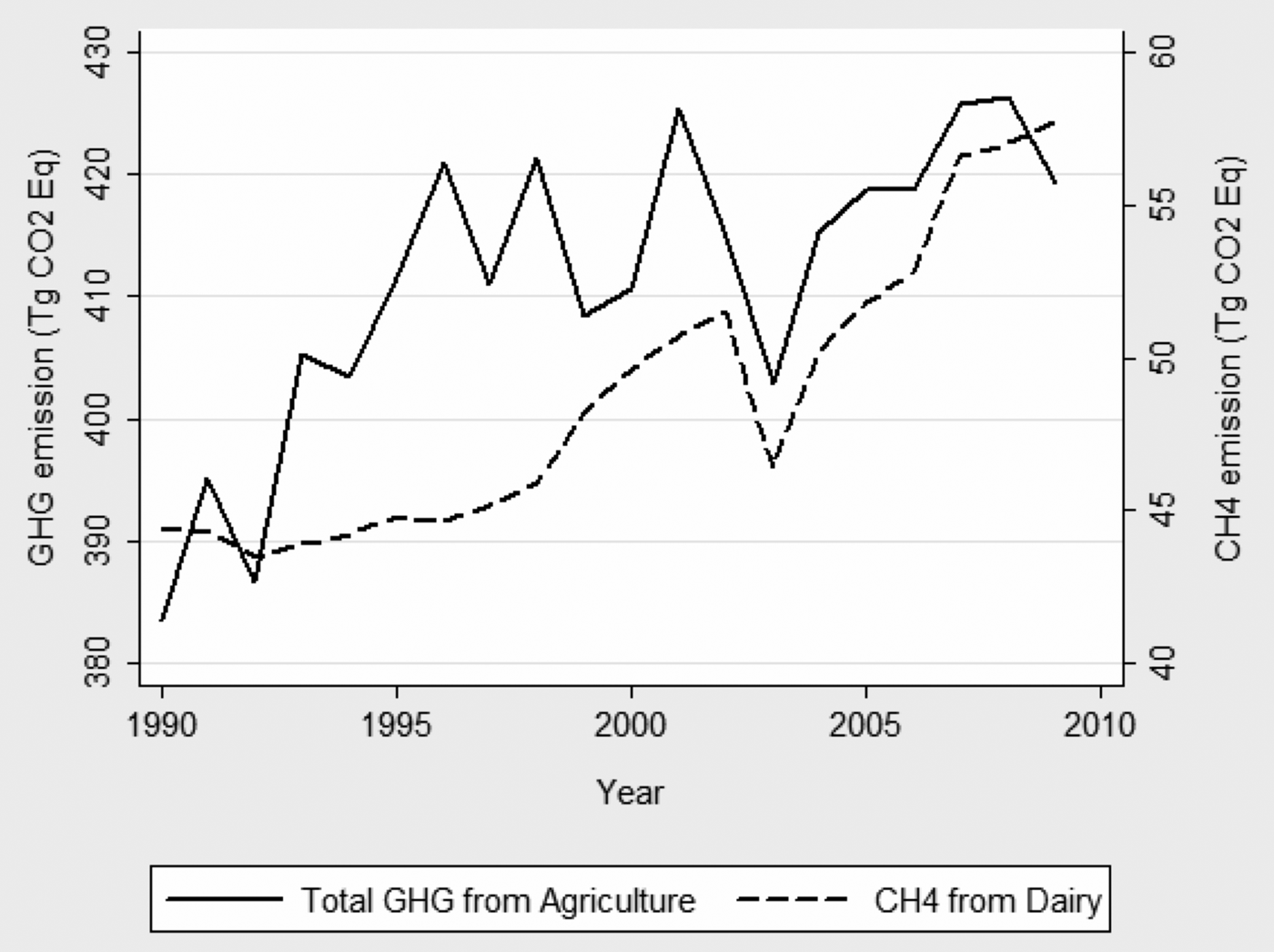
Benefits notwithstanding, the dairy sector in the Northeast faces serious challenges. Most notably, economies of scale and rapidly changing technologies are driving dairies to consolidate into larger operations at the expense of smaller family-operated farms. A national trend of fewer larger dairy farms has been observed for a number of years (MacDonald, McBride, and O'Donoghue Reference MacDonald, McBride and O'Donoghue2007); according to NASS (USDA 2010), the total number of dairy operations nationwide had decreased 83 percent since 1960. In addition, environmental problems created by pollution have raised concern about the industry's environmental sustainability (Thoma et al. Reference Thoma, Popp, Nutter, Shonnard, Ulrich, Matlock, Kim, Neiderman, Kemper, East and Adom2013). Dairy farms are responsible for generating pollutants such as carbon dioxide, methane, nitrogen oxide, ammonia, and acid gases (Environmental Protection Agency (EPA) 2012a). The greenhouse gas (GHG) emissions originating from dairy operations have been on an upward trend (EPA 2012a), accounting for 26 percent of total methane and 12 percent of total GHGs generated by the U.S. agricultural sector from 1990 through 2009 (EPA 2011). Figure 1 illustrates the evolution of methane emissions emanating from U.S. dairy farms.
Quantifying the environmental impact of GHGs poses various challenges. A key issue is that these GHGs, hereafter referred to as emissions, are not priced in markets, making it difficult to derive monetary measures of their environmental impacts. Moreover, these emissions have been termed “uniformly mixed assimilative pollutants” because they disperse from their point source of pollution over a large area and accumulate over time when the discharge rate exceeds the absorptive capacity of the environment (Tietenberg Reference Tietenberg2006). A consequence of these characteristics is that the sources of such pollution are difficult to inventory.
This study measures and analyzes environmental efficiency for groups of northeastern U.S. dairy operations that differ in size. Environmental efficiency analysis evaluates the tradeoff between production of a desirable good and associated emissions (Fernandez, Koop, and Steel Reference Fernandez, Koop and Steel2002). In this study, the first step in the analysis is construction of an emission index that incorporates the three major types of pollution emanating from dairy operations—livestock, fertilizer, and fuel—following Njuki and Bravo-Ureta (Reference Njuki and Bravo-Ureta2015). Thereafter, the joint production of the desirable output (dairy products) and emissions is analyzed to estimate the cost to society of those emissions as well as to establish whether environmental efficiency has improved or deteriorated over time.
Environmental Efficiency and Polluting Technologies
Over the years, productivity analyses have focused mainly on two major components, technical efficiency and technological change, while ignoring environmental efficiency. More recently, the interest in environmental efficiency has increased as evidenced by a number of studies (e.g., Chung, Färe, and Grosskopf Reference Chung, Färe and Grosskopf1997, Färe et al. Reference Färe, Grosskopf, Noh and Weber2005, Atkinson and Dorfman Reference Atkinson and Dorfman2005, O'Donnell Reference O'Donnell2007, Cuesta, Lovell, and Zofio Reference Cuesta, Lovell and Zofio2009). So far, however, work related to environmental efficiency in dairy farming has been limited; notable examples are Reinhard, Lovell, and Thijssen (Reference Reinhard, Lovell and Thijssen1999), Fernandez, Koop, and Steel (Reference Fernandez, Koop and Steel2002), Njuki and Bravo-Ureta (Reference Njuki and Bravo-Ureta2015), and Qi, Bravo-Ureta, and Cabrera (Reference Qi, Bravo-Ureta and Cabrera2015).
This study builds on recent developments in productivity analysis that have examined both desirable outputs and emissions (bad outputs) generated by a productive unit. This approach differs from previous work related to dairy farming in its construction and modeling of the pollution index. Whereas the environmental effects in studies by Reinhard, Lovell, and Thijssen (Reference Reinhard, Lovell and Thijssen1999) and Fernandez, Koop, and Steel (Reference Fernandez, Koop and Steel2002) were based only on the nitrogen surplus from fertilizer applications, the emission index constructed in this study also includes methane and nitrous oxide emissions from livestock and carbon dioxide emissions from fuel. According to Gerber et al. (Reference Gerber, Steinfeld, Henderson, Mottet, Opio, Dijkman, Falcucci and Tempio2013), feed production and processing are responsible for at least 45 percent of the GHGs emanating from livestock operations. Digestion by cows accounts for another 39 percent and manure decomposition accounts for 10 percent. The remainder of the emissions can be attributed to processing and transportation of animal products. Therefore, the emission index constructed in this study captures a sizable share of dairy operation emissions.
Researchers and stakeholders in the dairy sector became concerned about environmental efficiency in the Northeast because the EPA (2009) declared that GHGs posed a threat to public health and welfare and would be regulated under the Clean Air Act Amendment (1990),Footnote 2 which was meant to control three major threats to the environment: acid rain, urban pollution, and toxic air emissions. Specifically, EPA sought to control those environmental threats using economic incentives in a market-driven process that included performance-based standards and banking and trading of emissions. In its 2009 report, “Mandatory Reporting of Greenhouse Gases; Final Rule,” EPA provided a set of guidelines that would impose strict standards for reporting of GHG emissions in several sectors of the U.S. economy, including the livestock sector. Since implementation of the policy could have far-reaching implications, this analysis measures the impacts of emissions on the environmental efficiency of dairy farm operations in the northeastern United States.
Methodology
The theoretical foundation for modeling a multi-output technology is Shephard's (Reference Shephard1970) output-distance function (ODF). However, this function is not appropriate for modeling polluting technologies because it radially expands the desirable output and the emissions toward the frontier. Its proportional expansion of all outputs, good and bad, is not compatible with the goal of minimizing pollution.
An alternative to Shephard's ODF is the directional distance function developed by Chambers, Chung, and Färe (Reference Chambers, Chung and Färe1996) and later extended as a technique for modeling polluting technologies by Chung, Färe, and Grosskopf (Reference Chung, Färe and Grosskopf1997). Allowing the directional vectors for both inputs and outputs to vary generates a directional technology-distance function (Färe Reference Färe2010). In this study, the assumed technology follows previous studies that restricted the directional input vector to zero (e.g., Chung, Färe, and Grosskopf Reference Chung, Färe and Grosskopf1997, Färe et al. Reference Färe, Grosskopf, Noh and Weber2005, O'Donnell Reference O'Donnell2007). Hence, it is a directional output-distance function (DODF) that relies on two key assumptions: (i) in a multi-dimensional production frontier, the decision-making unit's (DMU's) objective is to simultaneously expand production of the desirable output and contract production of emissions; (ii) the directional vector can follow numerous projections to the frontier of the output set. The distance between the frontier and the observed output in the direction that reduces emissions while not decreasing the desirable output is the firm's environmental technical efficiency.
We begin by defining a technology as a technique, method, or process for transforming inputs into outputs. In addition, there are environmental factors, z ∈ ℜj+, that are exogenous and involved in the production process but are beyond the control of the DMU. The set of feasible combinations of inputs and outputs includes a vector of k inputs, x ∈ ℜk+, and vectors representing the desirable output and emissions, y ∈ ℜm+ and b ∈ ℜi+, respectively. Therefore, the environment-specific technology set can be defined (see O'Donnell Reference O'Donnell2016) as
 $$\eqalign{T\lpar z \rpar =& \lcub \lpar {x\comma \; y\comma \; b} \rpar \colon\, x \in {\Re_{+}^k} \comma \; y \in {\Re_{+}^m} \comma \; \cr & \quad b \in {\Re_{+}^i} \colon\, x \;{can \,produce} \lpar {y\comma \; b} \rpar \, {in \,environment}\; z\rcub .}$$
We also assume an output set, P(x, z) = {(y, b): (x, y, b) ∈ T(z)}, that is defined to be a multi-dimensional production-possibility frontier that represents the combination of production of the desirable output and of emissions (y, b) generated by the DMU using the input vector x in environment z. The output set satisfies standard production axioms (see Färe and Primont Reference Färe and Primont1995). In addition, we assume null-jointness—the good and the bad are produced jointly. Thus, if output of b is zero, it is not possible to generate any of good y (Shephard and Färe Reference Shephard and Färe1974). Following Shephard (Reference Shephard1970), we further assume that the outputs are weakly disposable such that any proportional amounts of contraction of the good and of the bad output are feasible. The weak disposability property implies that disposing of emissions is costly because some inputs must be redirected from producing the good output to emission reduction; that is, abatement requires a reduction in the firm's activity level (Kuosmanen Reference Kuosmanen2005).
When g = (g y, –g b) represents the directional vector, the environment-specific DODF is defined as
where x, y, and b are vectors of the inputs, the desirable output, and emissions respectively and z represents the exogenous environmental factors as already noted. We define β as a scaling factor, and the firm's objective is to expand production of the good output by βg y while contracting emissions by βg b. The directional vector is exogenously determined and hence can take a variety of values.
The properties of the DODF are inherited from the output set and can be specified as follows. First, the DODF is nonnegative for all feasible output vectors (y, b) ∈ P(x, z). Second, it is concave in (y, b) ∈ P(x, z). Third, it exhibits monotonicity, which corresponds to strong disposability of desirable outputs. This property is denoted as
According to equation 3, inefficiency does not increase if a firm, using the same amount of inputs, generates more of the good output and the same amount of the bad output. Under the fourth property, when the firm's production of emissions rises while production of the desirable output and of inputs remains constant, inefficiency does not decrease; that is (Färe et al. Reference Färe, Grosskopf, Noh and Weber2005),
The fifth property of the DODF is weak disposability for both goods, which can be expressed as
This equation indicates that a reduction in emissions requires a decrease in the firm's activity level (Kuosmanen Reference Kuosmanen2005). Finally, the sixth property is translation, which is analogous to homogeneity of degree one in Shephard's (Reference Shephard1970) output-distance function. The translation property is expressed as
 $$\eqalign{\mathop {D}^{\rightarrow}\! o\lpar x\comma z\comma \; y + {\rm \beta} {g_y}\comma \; b-{\rm \beta} {g_b}\semicolon \; {g_y}\comma-{g_b}\rpar &= \mathop {D}^{\rightarrow}\! o\lpar {x\comma \; z\comma \; y\comma \; b\semicolon \; {g_y}\comma \! -{g_b}} \rpar -{\rm \beta},\; \cr & \quad {\rm for}\; {\rm \beta} \in \Re.}$$
According to the translation property, the value of the resulting distance function will be more efficient by β if the vector of the good output expands by scaling factor βg y and the bad output contracts by βg b (Färe et al. Reference Färe, Grosskopf, Noh and Weber2005).
Figure 2 provides a graphical illustration of the DODF. The representative firm in this illustration initially produces inside the output set, P(x, z), at point A = (y 1, b 1). The objective is to increase the firm's efficiency by simultaneously expanding production of the desirable output and contracting production of emissions. This can be accomplished by scaling the vector from point A = (y 1, b 1) to point B = (y 1 + βg y, b 1 – βg b). The efficient combination of the desirable output and emission levels is determined by the tangency between the price ratio (p b/p y) and the frontier of the output set, P(x, z), at point B. Since emissions are not priced in markets, tangency of the price ratio and the frontier allows us to estimate their shadow price, p b. The vector g = (g y, –g b) represents the directional vector, which is determined exogenously following common practice (e.g., Chung, Färe, and Grosskopf Reference Chung, Färe and Grosskopf1997, Färe et al. Reference Färe, Grosskopf, Noh and Weber2005). By the translation property, the scaling of the vector from point A to point B parallel to the directional vector toward the frontier represents a solution to

Figure 2. Directional Output Distance Function
At the point of tangency, the representative firm has fully improved its environmental technical efficiency (ETE).
Empirical Specification
The parametric stochastic frontier takes the form
The last term represents a two-part disturbance that captures the unobserved firm effects, time-invariant persistent inefficiency, time-varying transient inefficiency, and random errors (the error specification is discussed in more detail hereafter).
A quadratic DODF is implemented while imposing values of g = (1, –1) on the directional vector, which represent equal weights assigned to the desirable output and desirable emissions. In addition, this choice of directional vector emphasizes the weak disposability property of the DODF previously discussed. That is, instead of scaling the directional vector from point A to the highest point of the output set (see Figure 2), a reduction in emissions requires a decrease in the firm's activity level. Moreover, the directional vector provides analytical simplicity and convenience in interpreting the results and is consistent with the related literature (e.g., Chung, Färe, and Grosskopf Reference Chung, Färe and Grosskopf1997, Färe et al. Reference Färe, Grosskopf, Noh and Weber2005, Picazo-Tadeo, Reig-Martinez, and Hernandez-Sancho Reference Picazo-Tadeo, Reig-Martinez and Hernandez-Sancho2005, Njuki and Bravo-Ureta Reference Njuki and Bravo-Ureta2015).
The model can be written as
 $$\eqalign{D \to o\lpar x\comma \; z\comma \; y\comma \; b\semicolon \; 1\comma \; - 1\rpar &= \alpha 0 + \sum\nolimits_{n = 1}^4 {{\alpha _n}} {x_{nit}} + \sum\nolimits_{n = 1}^2 {{\delta _n}} {z_{nt}} \cr & \quad + {\Pi _1}t + {\Pi _2}{t^2} + {{\rm \phi} _1}{y_{it}} + {{\rm \gamma} _1}{b_{it}} \cr & \quad + \displaystyle{1 \over 2}{{\rm \phi} _2}{y^2}_{1it} + \displaystyle{1 \over 2}{\gamma _2}{b^2}_{it} + \lpar {\omega _i} + {\varepsilon _{it}}\rpar .} $$
The variable xnit represents conventional inputs: cows, capital, labor, and purchased feed respectively. Intermediate materials used in the production process are embedded in capital. The variable znt captures 30-year moving averages of two climate variables, temperature and precipitation. The variables t and t 2 represent a linear and a quadratic time trend that capture technical change in the model;Footnote 3 and, finally, yit and bit measure milk output and emissions respectively. For the translation property to hold and to account for the choice of the directional vector, we impose the parametric restriction ϕ1 – γ1 = –1 (Färe et al. Reference Färe, Grosskopf, Noh and Weber2005).
Recent studies have developed a four-way error structure to disentangle unobserved firm effects, time-invariant persistent technical efficiency, time-varying transient technical efficiency, and random errors (e.g., Colombi et al. Reference Colombi, Kumbhakar, Martini and Vittadini2014, Filippini and Greene Reference Filippini and Greene2014, Kumbhakar, Lien, and Hardaker Reference Kumbhakar, Lien and Hardaker2014, Tsionas and Kumbhakar Reference Tsionas and Kumbhakar2014). In the dairy sector, persistent inefficiency levels can arise from institutional and statutory regimes such as minimum pricing laws and food and safety regulations. Transient inefficiency levels, on the other hand, are derived from shocks associated with implementing new technologies (Kumbhakar, Tsionas, and Sipilainen Reference Kumbhakar, Tsionas and Sipilainen2009) and human capital (Kumbhakar, Ghosh, and McGuckin Reference Kumbhakar, Ghosh and McGuckin1991). Furthermore, unobserved firm effects come about because firms adjust their use of inputs in response to constantly changing production environments, a process that is observed by the producer but not by the econometrician (Kellerman Reference Kellerman2015).
Following Filippini and Greene (Reference Filippini and Greene2014), we employ a generalized true random effects (GTRE) approach that nests the pooled frontier and true random effects models. Consequently, the error structure in equation 7 (ωi + εit) is a two-part disturbance. The first part, ωi = ξi – ηi, is a time-invariant component in which ξi captures firm heterogeneity and ηi captures persistent technical inefficiency. This component follows a skew-normal distribution and has distributional parameters of κ = ση/σξ and θ = (ση2 + σξ2)1/2. The second part, εit = v it – u it, is a time-varying component. The term vit represents statistical error that captures measurement errors and functional form errors, and uit represents transient technical inefficiency. This component also follows a skew-normal distribution with parameters λ = σu / σv and ρ = (σv2 + σu2)1/2.
As in Färe et al. (Reference Färe, Grosskopf, Noh and Weber2005), we assume that, for the ith observation, the scaling factor βi is added to yi and subtracted from bi. We set βi = bi. Thus, we obtain variation on the lefthand side by choosing a specific βi for each observation. The functional form given in equation 7 can now be rewritten as
 $$\eqalign{-\lpar {emissions} \rpar &= {{\rm \alpha }_0} + {{\rm \alpha }_1}cows_{it} + {{\rm \alpha }_2}capital_{it} + {{\rm \alpha }_3}labor_{it} + {{\rm \alpha }_4}feed_{it} \cr & \quad + {{\rm \delta }_1}temp_t + {{\rm \delta }_2}prec_t + {{\rm \pi }_1}time_t + 1/2{{\rm \pi }_2}time_t^2 + {{\rm \varphi }_1}milk_{it} \cr & \quad + 1/2{{\rm \varphi }_2}milk_{it}^2 + 1/2{{\rm \gamma }_2}emissions_{it}^2 + \lpar {{\rm \omega }_i} + {{\rm \varepsilon }_{it}}\rpar .}$$
Shadow Prices and Morishima Elasticities of Output Substitution
The shadow price is defined as the dollar value of the emission output generated at the tangency of the price line (p b/p y) and the output frontier (P x). The shadow price also can be defined as the marginal abatement cost and can be calculated by setting up the revenue function following Chambers, Chung, and Färe (Reference Chambers, Chung and Färe1998):
where p y is the price of the desirable output, p b is the price of the emissions, and D →o(x, z, y, b; g y, –g b) is the directional output-distance function. The Lagrangian expression associated with maximization of revenue subject to the DODF is
To solve for the revenue function, we need to establish the value of λ. By making use of the translation property, the revenue function can be rewritten as
 $$\eqalign{R \lpar{\,p_y}\comma \; {\,p_b}\semicolon \; {\rm \beta} \rpar &= {\rm max}_{y\comma \; b} \lcub {\,p_y}\lpar y + {\rm \beta} {g_y} \rpar - {\,p_b} \lpar b + {\rm \beta} {g_b} \rpar \colon \cr & \quad \mathop {D}^{\rightarrow}\! o \lpar {\it x}\comma \; z\comma \; y\comma \!+\! {\rm \beta} {g_y}\comma \; b \!+\! {\rm \beta} {g_b}\semicolon \; {g_y}\comma-{g_b}\rpar \!\ge\! 0\rcub + {\rm \beta} \lpar{\,p_y}{g_y} \!+\! {\,p_b}{g_b}\rpar .} $$
The short form of this revenue function is
which implies that
By incorporating the translation property into the Lagrangian expression, we obtain
Then, we apply the envelope theorem to arrive at
Using the initial values for the directional vector (1, –1), we solve for the revenue function:
 $$\eqalign{R\lpar {{p_y}\comma \; {p_b}\semicolon \; 1\comma \; -1} \rpar & = {\rm max}_{y\comma \; b} \lcub {p_y}\cdot \,y - {p_b}\cdot \,b\colon ({p_y}\cdot \,1 + {p_b}\cdot \,1)\cr & \quad \times \mathop {D}^{\rightarrow} o\lpar {x\comma \; z\comma \; y\comma \; b\semicolon \; 1\comma \; -1} \rpar \rcub.}$$
The first-order conditions associated with the revenue function are
and
The ratio from those expressions gives the relative shadow price as
We turn next to the Morishima elasticity of substitution (MES), which Blackorby and Russell (Reference Blackorby and Russell1989, p. 883) defined as “a measure of curvature, or ease of substitution.” More recently, Färe et al. (Reference Färe, Grosskopf, Noh and Weber2005) defined the MES as a measure of the change in the ratio of the price of the desirable output to the price of the emissions relative to a change in the quantity of the desirable output and emissions:
In our case, the MES is an indicator of the ability of the dairy operation to trade reductions in milk for reductions in emissions. Based on the DODF used in our model, the MES can be specified as
 $$\eqalign{MES_{by}&=y\left[{\partial ^2 {\mathop {D}\limits^{\rightarrow}} o\lpar x\comma \; z\comma \; y\comma \; b\semicolon \; 1\comma \; -1 \rpar /\partial b^2 \over \partial {\mathop {D}\limits^{\rightarrow}} o\lpar x\comma \; z\comma \; y\comma \; b\semicolon \; 1\comma \; -1 \rpar / \partial b} \right. \cr & \quad \left. -{\partial ^2 {\mathop {D}\limits^{\rightarrow}} o\lpar x\comma \; z\comma \; y\comma \; b\semicolon \; 1\comma \; -1 \rpar /\partial y^2 \over \partial {\mathop {D}\limits^{\rightarrow}} o\lpar x\comma \; z\comma \; y\comma \; b\semicolon \; 1\comma \; -1 \rpar / \partial y}\right]}$$
Data
The data set used in this analysis is derived from annual publications prepared by Farm Credit East (FCE), a financial institution and specialized lender that caters to farm businesses in the Northeast. These annual publications assess the financial health and progress of dairy farm businesses. Our data set covers dairy operations located in Connecticut, Maine, Massachusetts, New Hampshire, Rhode Island, Vermont, and New York and spans the 34-year period of 1980 through 2013. The dairies covered in the reports received most of their incomes from milk sales; between 2009 and 2013, for example, milk sales represented 83.2–88.3 percent of the aggregate annual income received by the dairies.
To preserve confidentiality, the FCE does not make individual farm-level data available. Instead, the data are aggregated and averaged at the farm level and reported on an annual basis for four categories of herd size. Hence, the units of observation in this study correspond to those categories. For the 34-year period covered by the data, we obtained 136 observations (dairies) that we grouped into small dairies, which had fewer than 90 cows; medium dairies, which had 90 to 149 cows; large dairies, which had 150 to 299 cows; and very large dairies, which had 300 or more cows. The number of dairies that participated in the annual survey ranged from 391 in 1980 to 789 in 1992.
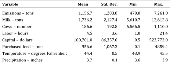
Descriptive statistics for the variables in the data set are outlined in Table 1. The quantity of feed purchased was constructed by dividing nominal figures for total feed expense per cow by the nominal price for a 16-percent feed concentrate per year using prices obtained from the New England regional office of NASS. The variable for labor, expressed in worker-equivalent-hours, was collected and summarized by the FCE. All monetary values were converted to constant 2013-dollar values using the producer price index derived from the Bureau of Labor Statistics.
Table 1. Descriptive Statistics

Next, the data were augmented with estimates of emissions using a comprehensive pollution index and climate variables that consisted of 30-year moving averages of daily regional temperature and precipitation derived from the National Oceanic and Atmospheric Administration. These were included in the model in response to evidence that variations in climate affect dairy production activities (e.g., Mukherjee, Bravo-Ureta, and De Vries Reference Mukherjee, Bravo-Ureta and De Vries2013, Key and Sneeringer Reference Key and Sneeringer2014, Njuki and Bravo-Ureta Reference Njuki and Bravo-Ureta2015, Qi, Bravo-Ureta, and Cabrera Reference Qi, Bravo-Ureta and Cabrera2015). The large size of the numerical values of the outputs and inputs resulted in convergence difficulties; thus, following Färe et al. (Reference Färe, Grosskopf, Noh and Weber2005), we normalized the data by dividing each output and input value by its mean value before estimating equation 8.
Construction of the Undesirable Output
As previously noted, a recent report by Gerber et al. (Reference Gerber, Steinfeld, Henderson, Mottet, Opio, Dijkman, Falcucci and Tempio2013) indicated that a significant share of GHGs emanating from livestock operations can be attributed to feed production and processing, digestion by cows, and manure decomposition. By constructing an index that captures emissions associated with livestock, fuel, and fertilizer, we account for a significant share of the emissions generated by the milk production portion of the fluid milk supply chain.
The index of emissions from fuel is constructed using data on each dairy's expenditures for gasoline and oil. Expenditures are converted to quantities of fuel consumed in gallons based on historical data on conventional gasoline prices from the U.S. Department of Energy's Energy Information Administration, and the equivalent emissions of carbon dioxide from those fuels are computed using the EPA's GHG equivalencies calculator (EPA 2012b).
The index of fertilizer-based emissions is constructed using information on the dairies’ fertilizer expenditures and historical fertilizer prices from NASS to convert the expenditures to quantities. The amount of direct emission of nitrous oxide, which is derived from nitrogen applied to the soil via fertilizers, is calculated using formulations by Mosier (Reference Mosier1994).
For the livestock-based emissions, we use methodologies outlined in EPA guidelines (2009, p. 56481)Footnote 4 that were designed to improve the accuracy of information collected regarding GHG emissions and to better understand the sources of those emissions. These guidelines were authorized by congress under the Consolidated Appropriations Act (2008). The livestock component of the emissions index is measured in metric tons of carbon dioxide equivalent, which accounts for methane and nitrous oxide generated by animals at dairy facilities. The amount of methane emitted is a product of total volatile solids (VS) excreted per animal (which varies with the type of animal), the fraction of the VS that is methane (also varies by animal type), and a conversion factor for the global warming potential of methane.
Total VS is a product of the average annual animal population at the facility, the typical mass of each animal type (for dairy cows, the default value is 604 kilograms (kg)), and the VS excretion rate for type of animal, which varies by state. In the northeast United States, these rates range from 8.63 VS per day per 1,000 kg of animal mass in Massachusetts to 9.44 VS per day per 1,000 kg of animal mass in New Hampshire. We use the average for the region, 9.09. The resulting estimates of methane produced are then multiplied by 21, the global warming potential of methane. We compute the amount of livestock-based nitrous oxide emissions using the same calculations. The daily nitrogen excretion rate for the northeastern United States ranges from 0.51 VS per day per 1,000 kg of animal mass in Massachusetts to 0.54 kg of VS per day per 1,000 kg of animal mass in New Hampshire. We use the average for the region, 0.525. The resulting estimates of nitrous oxide produced are then multiplied by the conversion factor of 310 to determine the potential for global warming.
The combination of these three major sources of pollution determines total emissions. Table 1 provides a summary of the variables used in the analysis.
Results
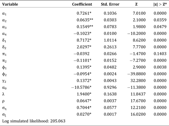
Table 2 presents the estimated coefficients, standard errors, and results of the distributional parameters: λ, ρ, ση, and σξ. The estimated coefficients are then used to compute shadow prices and Morishima elasticities of substitution.
Table 2. Estimated Random Coefficients from the Frontier Model

Note: * denotes significance at the 1 percent level, ** at the 5 percent level, and *** at the 10 percent level.
In terms of the distributional parameters, the ratio of σu to σv is denoted by λ. This ratio signifies the relative importance of the transient inefficiency term u it with respect to the two-sided statistical error term v it. The estimated value of λ is 1.94, which implies that the one-sided transient inefficiency component dominates any statistical error in determination of the time-varying component, εit. The variance of the persistent inefficiency term ση, on the other hand, is 0.70 and dominates the variance of the farm-size heterogeneity term σξ, 0.03. Hence, we conclude that the persistent inefficiency term largely determines the composition of the time-invariant component ωi.
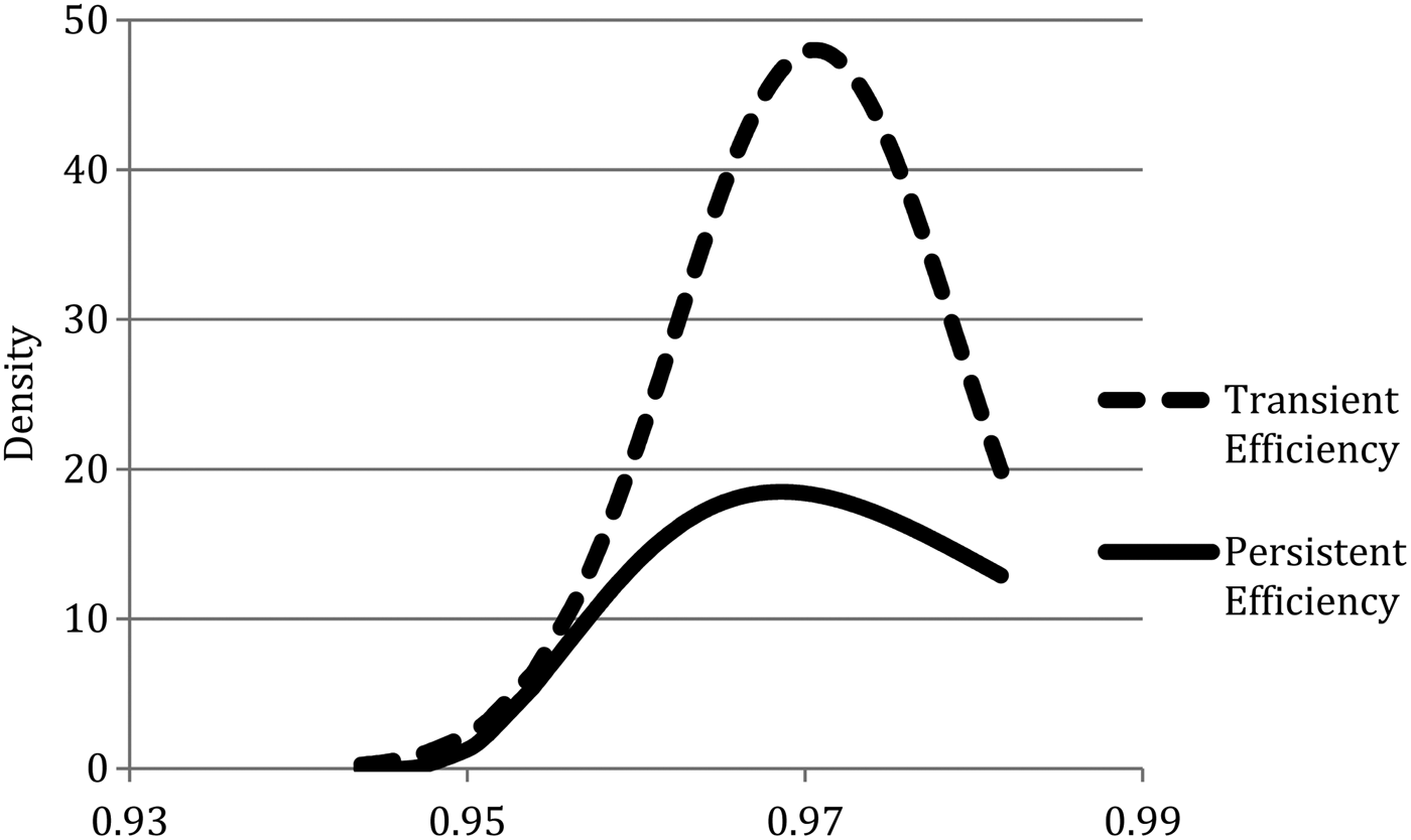
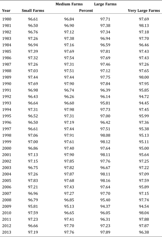
Tables 3 and 4 report the estimates of transient and persistent technical efficiency by farm size. The kernel densities for the efficiency estimates are plotted in Figure 3. These estimates are higher on average than ones of technical efficiency from studies of the stochastic production frontier for U.S. dairies (e.g., Ahmad and Bravo-Ureta Reference Ahmad and Bravo-Ureta1996, Bravo-Ureta et al. Reference Bravo-Ureta, Solis, Moreira, Maripani, Thiam and Rivas2007). Moreover, farm size has no notable effect on efficiency.

Figure 3. Kernel Density for Persistent (long-run) and Transient (short-run) Technical Efficiency
Table 3. Transient Technical Efficiency

Table 4. Persistent Technical Efficiency

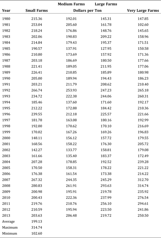
Table 5 reports the estimated shadow prices. To illustrate the meaning of the shadow price in this context, consider the $215.4 value for small farms in 1980. This shadow price indicates that an increase in milk output at the margin would have generated an additional $215.4 worth of emissions. Alternatively, this is the dollar value that the average small farm would have had to forfeit in 1980 to reduce emissions by one ton.
Table 5. Shadow Prices

In terms of farm size, our results are mixed. The lowest estimated shadow price is $102.6 for very large farms in 1981. On the other hand, the highest estimated shadow price is $314.7 in 2008, again for very large farms. In general, at the beginning of the sample period, small farms consistently faced the highest shadow prices. However, beginning in the mid-1990s, the estimated shadow prices for very large farms began to exceed those of smaller farms. Thus, larger operations would have faced greater marginal abatement costs relative to their smaller counterparts.
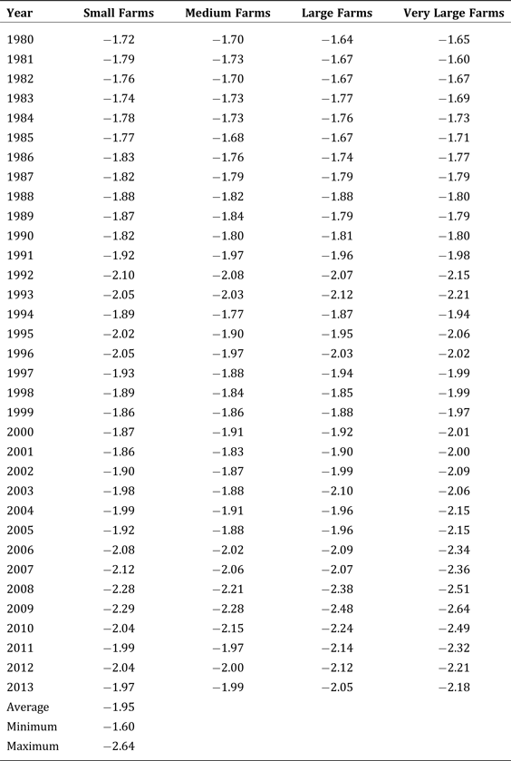
As previously mentioned, the MES evaluates the ability of a dairy operation to trade reductions in milk output for reductions in emissions. We present the MES estimates by farm size in Table 6. In the early years, the estimates are highest for small dairy operations in absolute value. Once again, however, the situation changes in the mid-1990s, and the MES estimates of very large dairy farms begin to exceed those of other dairy operations. In addition, we find evidence that, in general, the MES values trend upward over time regardless of the size of the operations, which points to a reduction in the ability of dairies to make the substitution and curb their emissions in recent years.
Table 6. Morishima Elasticity of Substitution

Concluding Remarks
This study evaluates environmental efficiency for northeastern U.S. dairy farms of various sizes. Using data derived from Farm Credit East for 1980 through 2013, we estimate a directional output-distance function that measures joint production of milk and emission of GHGs while incorporating a four-way error approach that accounts for unobserved farm-size heterogeneity, time-varying transient technical efficiency, time-invariant persistent technical efficiency, and random errors. We also estimate shadow prices and output elasticities related to the cost of reducing emissions.
In terms of technical efficiency, we find that farm size has no significant effect. However, the computed shadow prices and output elasticities indicate that, beginning in the mid-1990s, very large dairy operations faced higher shadow prices and MES values relative to other farms, and in later years, we find that the output elasticities generally trended up for all farm sizes.
As noted, the dairy industry both nationwide and in the Northeast has been consolidating (USDA 2014, Winsten et al. Reference Winsten, Kerchner, Richardson, Lichau and Hyman2010). Among the benefits of larger dairy operations are economies of scale, increased productivity (Mosheim and Lovell Reference Mosheim and Lovell2009), and a higher cash margin per unit of milk sold (MacDonald, McBride, and O'Donoghue Reference MacDonald, McBride and O'Donoghue2007). In recent years, large dairy operations in the Northeast have been characterized by confinement of large herds in relatively small and restricted areas. These confinement-feeding systems have been adopted to reduce production costs and raise the output of milk per cow (Winsten et al. Reference Winsten, Kerchner, Richardson, Lichau and Hyman2010). However, having large herds in a confined area contributes to higher levels of emissions since the cows are kept and raised in restricted lots rather than on rangeland and pasture.
According to Farm Credit East, 65 of the 517 farms surveyed in 2013 maintained more than 700 cows. Dairy operations of that size are required to meet statutory environmental standards under the Clean Water Act of 1972 and rules regarding concentrated animal feeding operations (EPA 2008) that seek to protect the quality of ground water and public health. As a result, these large dairy farms would have been required to obtain manure discharge permits and to develop nutrient management plans to minimize the negative effects of animal waste (Tao et al. Reference Tao, Morris, Bravo-Ureta, Meinart and Neafsey2012). These requirements may have raised the cost of manure management and, hence, shadow prices, and the difficulty associated with reducing emissions while maintaining or raising the output of milk would then be reflected in higher MES values.
Our results suggest that any policy action taken to curb emissions could adversely affect the competitiveness of large-scale dairy operations. This poses a significant dilemma for policymakers given the importance of dairy farming to local economies and preservation of agricultural landscapes in the Northeast (Johnston Reference Johnston2002). We propose that public policy interventions be directed toward large dairy operations to assist them in improving their environmental efficiency and to smaller dairy farms to assist them in becoming environmentally sustainable as they expand. These types of assistance could take various forms, including an emphasis on extension services that could provide expert advice regarding ways to reduce pollution and direct subsidies and tax breaks for farms that install pollution-reduction equipment such as anaerobic digesters.


