Online gait learning with Assist-As-Needed control strategy for post-stroke rehabilitation exoskeletons

Abstract

Lower limb exoskeletons (LLEs) have demonstrated their potential in delivering quantified repetitive gait training for individuals afflicted with gait impairments. A critical concern in robotic gait training pertains to fostering active patient engagement, and a viable solution entails harnessing the patient’s intrinsic effort to govern the control of LLEs. To address these challenges, this study presents an innovative online gait learning approach with an appropriate control strategy for rehabilitation exoskeletons based on dynamic movement primitives (DMP) and an Assist-As-Needed (AAN) control strategy, denoted as DMP-AAN. Specifically tailored for post-stroke patients, this approach aims to acquire the gait trajectory from the unaffected leg and subsequently generate the reference gait trajectory for the affected leg, leveraging the acquired model and the patient’s personal exertion. Compared to conventional AAN methodologies, the proposed DMP-AAN approach exhibits adaptability to diverse scenarios encompassing varying gait patterns. Experimental validation has been performed using the lower limb rehabilitation exoskeleton HemiGo. The findings highlight the ability to generate suitable control efforts for LLEs with reduced human-robot interactive force, thereby enabling highly patient-controlled gait training sessions to be achieved.

1. Introduction

Robotic lower limb exoskeletons (LLEs) have been developed to facilitate quantified repetitive gait training for individuals afflicted with gait impairments stemming from Spinal Cord Injury [1, 2], stroke [3, 4], and cerebral palsy [5, 6]. Over the past few decades, LLEs have gained widespread utilization in supporting therapy and enhancing the efficiency of rehabilitation processes. Nevertheless, certain challenges persist in the domain of post-stroke rehabilitation.

For patients recovering from stroke, the severity of their disability not only varies among individuals but also fluctuates during the course of training [7]. As shown in Fig. 1, various types of gait training, namely passive, active-assistive, active, and resistive, are employed at different stages of rehabilitation to accommodate different states of bodily recovery [8], where the blue arrow denotes the direction of patient movement, while the red arrow represents the movement of the exoskeleton robot. The ticked solid arrows signify the active movements and the blue arrows with a cross signify the inactive movements. Note that the passive training is administered during the initial phase of rehabilitation when patients possess limited muscle strength, whereas resistive training is employed during the final stage when patients exhibit sufficient muscle strength. It is widely postulated that active engagement and voluntary participation of patients in gait training could yield favorable outcomes and expedite the recovery process [9, 10]. Consequently, one critical issue of gait training is to encourage high levels of patient involvement.

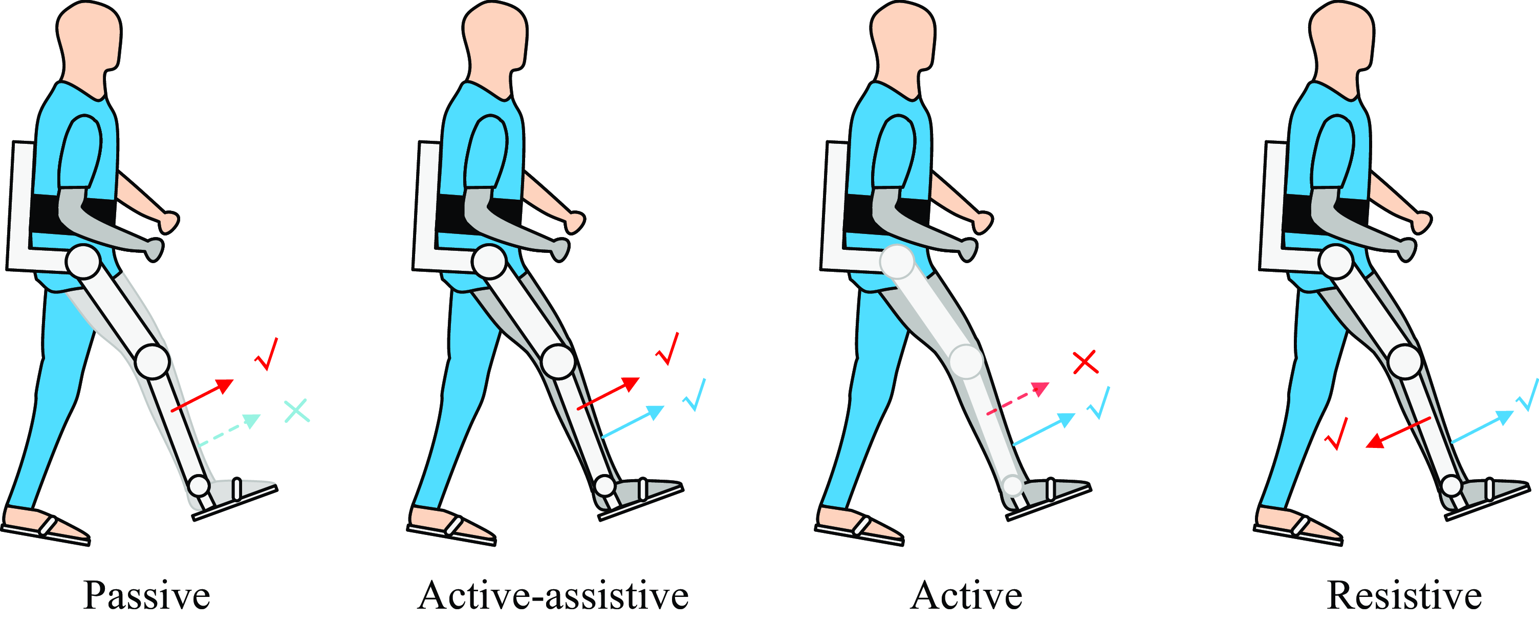
Figure 1. Four types of gait training. The red arrow represents the moving direction driven by the exoskeleton robot, and the blue arrow represents the patient’s own moving direction. The tick and the cross indicate the active and inactive movement, respectively. For instance, for the Passive gait training, the patient is with no active movement, and the exoskeleton is moving the patient’s leg forward actively.

In recent years, there has been a notable application of Assist-As-Needed (AAN) control strategies in implementing the aforementioned four types of gait training through a unified approach. AAN control encompasses various categories, such as impedance control, model-based control, and field-based control approaches. Impedance/admittance-based AAN controllers have been extensively investigated in upper limb rehabilitation robots [11, 12], LLEs [13], and ankle rehabilitation robots [14]. Specifically, for LLEs, impedance control has been employed in diverse assistance applications, including sit-to-stand tasks [15], gait training [13], and load carrying [16]. In the realm of model-based control approaches, Caulcrick et al. [8] proposed a model predictive control (MPC) architecture for LLEs, where the human residual torque is estimated from electromyography signals, the joint torques are predicted by MPC, and the assistance mode is selected by fuzzy logic algorithms. For field-based control, the basic idea is to construct an artificial potential field around the reference position or velocity trajectory and force the robot to move around them, including force field control in Cartesian space [17], velocity field control in Cartesian space [18], and path control in joint space [19].

Existing AAN algorithms commonly rely on fixed predefined gait patterns obtained from healthy subjects as reference trajectories. However, due to the inherent variability in gait patterns among patients, it becomes challenging to generate suitable patterns for each patient using a single predefined trajectory. Notably, post-stroke patients often exhibit the ability to voluntarily move their unaffected leg (healthy leg), thereby enabling the collection of joint angle data from the healthy leg to serve as a reference for the paretic leg [20–22]. Consequently, the unresolved challenge lies in effectively utilizing the collected joint angles from the healthy leg, along with the residual muscle strength of the paretic leg, to facilitate individualized gait training.

In light of the above, this study aims to investigate gait training using LLEs specifically for post-stroke patients presenting primarily with weakness and no spasticity. To construct the online gait learning framework, Dynamic Movement Primitives (DMP) are adopted [23], given their efficacy in motion planning for robot arms [24] and gait planning for exoskeleton robots [25–27]. Leveraging DMP, joint angles from the healthy leg can be dynamically learned in real-time for each individual step, empowering patients to guide the movement of the paretic leg and exert control over gait patterns. To harness the residual muscle strength of the patient, an AAN approach is implemented to control the active leg of the exoskeleton. The primary contributions of this research can be summarized as follows:

• Proposal of an online gait learning framework for post-stroke rehabilitation exoskeletons, enabling LLEs to acquire real gait patterns on a step-by-step basis;

• Integration of dynamic movement primitives (DMP) and the AAN algorithm to develop a patient-controlled gait training methodology that overcomes the limitations associated with the conventional AAN approach employing a predefined trajectory.

Consequently, the proposed approach enables patients to engage in individualized gait training with varying patterns instead of being restricted to a fixed predefined trajectory. Furthermore, it promotes high levels of active involvement on the part of the patients.

2. DMP-AAN control approach

In this section, we shall introduce the DMP-based online gait learning methodology as well as the AAN control approach, hereby referred to as the DMP-AAN control approach. The following subsections are introduction of the framework of the proposed approach, the gait learning, and the detailed equations for impedance model and the guide model in the AAN control approach, respectively.

2.1. Framework of the DMP-AAN control approach

The framework of the approach is visually presented in Fig. 2, encompassing two integral components: the gait learning approach and the AAN control strategy. Notably, the gait learning approach is distinguished by a light green background color, while the AAN control strategy is depicted with a light red background color.

Figure 2. Framework of the DMP-AAN control approach, where $\theta _{\mathrm{hh}}$ and $\theta _{\mathrm{hk}}$ are hip and knee joint angles sampled from the healthy leg, $\theta _{\mathrm{act}}=[\theta _{\mathrm{ph}}$ , $\theta _{\mathrm{pk}}]$ are hip and knee joint angles from the paretic leg. The exoskeleton’s passive leg without motors is strapped to the healthy leg of the patient (the left leg), and the exoskeleton’s active leg with motors is strapped to the paretic leg of the patient (the right leg). $F_L$ and $F_R$ are ground reaction force for the left and right foot, respectively.

2.1.1. Gait learning

Given the attachment of the exoskeleton legs to the patient’s legs, the joint angles can be effectively captured through the utilization of joint angle encoders, which are integrated within the hip and knee joints of the exoskeleton legs. It is noteworthy that the passive leg of the exoskeleton lacks motors and operates on a fully back-driven mechanism, thereby permitting unrestricted movement of the leg by the patient. Furthermore, depending on the paretic side of the patient, the left and right leg of the exoskeleton can be substituted with a passive or active leg. The trajectory learning process for each leg can be segregated into two fundamental phases within each gait cycle: the support phase and the swing phase. The determination of the support and swing phases can be facilitated through the evaluation of ground reaction forces, whereby the force sensors embedded in the exoskeleton’s insoles allow for the measurement of the ground reaction forces exerted on the left foot ( $F_L$ ) and the right foot ( $F_R$ ).

2.1.2. AAN control

The acquisition of the reference joint angles for the paretic leg can be achieved through the process of learning from the corresponding joint angles of the healthy leg. Concurrently, the current joint angles of the paretic leg can be accurately assessed via the implementation of joint angle sensors embedded within the hip and knee joints. Leveraging the current and reference joint angles, the AAN control approach can be effectively executed.

2.2. DMP-based online gait learning

For the gait trajectory learning component, the joint angles are learned and reproduced by the DMP [23]. Since the gait trajectory is learned for each individual step rather than the entire gait cycle, the discrete DMP is employed, which can be expressed as follows:

(1) \begin{equation} \lambda ^2 \ddot \theta = \alpha (\beta (\theta _g-\theta )-\lambda \dot \theta ) + P(f - x (\theta _g-\theta _0)), \end{equation}

where $\lambda$ is a time constant for time tunning of the reproduced trajectory. $[\theta, \dot \theta, \ddot \theta ]$ is the joint angle, joint angular velocity, and joint angular acceleration, respectively. $\theta _0$ and $\theta _g$ are the initial and desired joint angles, respectively. $\alpha$ and $\beta$ are constant parameters, $P$ is also a constant value, and $P=\alpha \beta$ . $f$ is a non-linear forcing term for the trajectory profile modeling, which can be calculated as:

(2) \begin{equation} f(x)=\frac{\sum _{i=1}^{N} \Psi _{i}(x) w_{i} x}{\sum _{i=1}^{N} \Psi _{i}(x)}, \end{equation}

where $N$ is the number of basis functions, $x$ is determined by a first-order canonical system: $\lambda \dot x = - \gamma x$ . $\Psi _i$ is basic functions, which can be calculated as:

(3) \begin{equation} \Psi _{i}(x) = \exp \left (-\frac{1}{2 \sigma _{i}^{2}}\left (x-c_{i}\right )^{2}\right )\!, \end{equation}

where $\sigma _i$ and $c_i$ are respectively variations and centers for basis function $\Psi _{i}$ . For the learning phase of DMP, the non-linear forcing term $f_d$ can be calculated as:

(4) \begin{equation} f_{\text{d}}=\frac{\lambda ^2 \ddot \theta _{\text{d}} - \alpha (\beta (\theta _g-\theta _{\text{d}})-\lambda \dot \theta _{\mathrm{d}})}{P} + x(\theta _g-\theta _0). \end{equation}

where $\theta _{\text{d}} = [\theta _{\text{hh}}, \theta _{\text{hk}}]$ are the demonstrated joint angles sampled from the healthy leg. $\dot \theta _{\text{d}}, \ddot \theta _{\text{d}}$ are the first- and second-order derivatives of $\theta _{\text{d}}$ . To find the corresponding $w_i$ for basic function $\Psi _{i}$ , construct the loss function:

(5) \begin{equation} J_i = \sum ^N_{t=1} \Psi _i(t) (f_{\text{d}}(t) - w_i \xi (t))^2 \end{equation}

where $\xi (t) = x(t)(\theta _g - \theta _0)$ . The learning of $w_i$ is accomplished with locally weighted regression [23].

2.3. AAN control strategy

AAN control can be realized through the utilization of an impedance model and a guide model. The impedance model enforces the movement of joint angles within an artificial virtual tunnel, while the guide model directs the joints to progress along the reference joint angles, as illustrated in Fig. 3. The reference torque $\tau _{\mathrm{ref}}$ applied to the joints of the exoskeleton can be denoted as:

(6) \begin{equation} \tau _{\mathrm{ref}} = \tau _{\mathrm{c}} + \tau _{\mathrm{i}} + \tau _{\mathrm{g}}, \end{equation}

where $\tau _{\mathrm{c}}$ is for gravity and friction compensation, which can be calculated with the sensor data (joint angles and angular velocities, etc.) from the exoskeleton robot. $\tau _{\mathrm{i}}$ is the torque in impedance control for joint angle correction. $\tau _{\mathrm{g}}$ is the guiding torque to guide the joint forward along the reference trajectory. In this paper, $\tau _{\mathrm{i}}$ and $\tau _{\mathrm{g}}$ are calculated by the impedance model and the guide model, respectively.

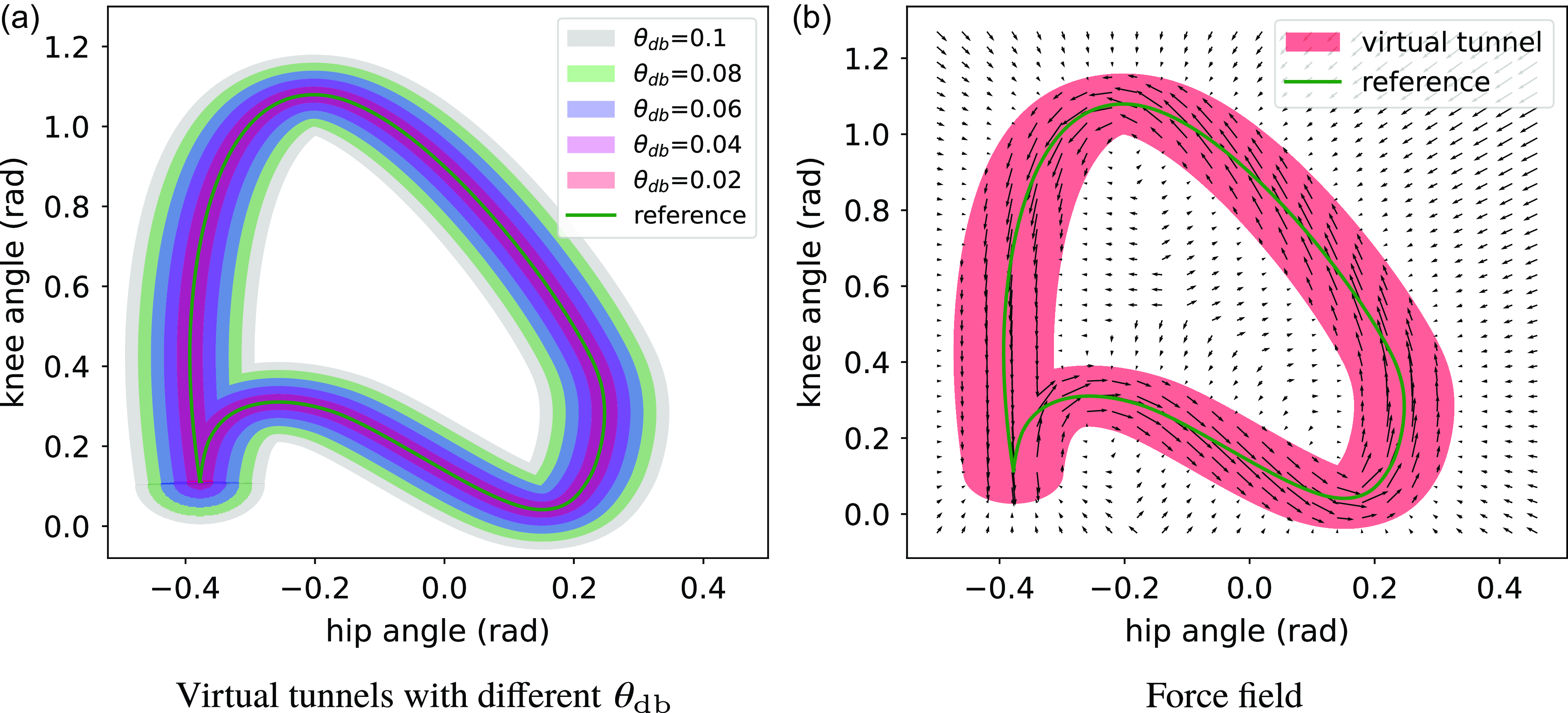
Figure 3. Schematic of the virtual tunnel and force field created by AAN approach, where the assistant torque is tangential along the reference trajectory in the virtual tunnel, and normal to the reference trajectory outside the virtual tunnel.

Let us denote $\theta _{\mathrm{ref}}(S)$ as the demonstrated joint angle sampled from the healthy leg, where $S$ is the index set of the gait cycle, which is normalized to the interval $[0,T)$ . $S$ is calculated by the modulo operation with respect to $T$ :

(7) \begin{equation} S(t) = t\ {mod} \ T, \end{equation}

where $t$ is time, $T$ is the duration of either the support phase or the swing phase of the healthy leg while sampling joint angles from it. Note that $S(0)=0$ denotes the start of the demonstrated joint angle, $S(T) \rightarrow T$ denotes the last data point of the demonstrated joint angle, that is, the end of the support gait phase or swing gait phase. For the current actual joint angle, index $s$ is not a function of time, it is determined by the distance between the actual joint angle and the reference joint angle, which is defined as:

(8) \begin{equation} s^*= \mathop{\mathrm{arg\,min}}\limits_{s \in S} \| \theta _{\mathrm{ref}} - \theta _{\mathrm{act}} \|^2, \end{equation}

where $\theta _{\mathrm{ref}} = [\theta _{\mathrm{hh}}, \theta _{\mathrm{hk}}]$ is the joint angles sampled from the healthy leg in the last support or swing gait phase. $\theta _{\mathrm{act}} = [\theta _{\mathrm{ph}}, \theta _{\mathrm{pk}}]$ is the current actual joint angles from the paretic leg. $s$ is determined by the Euclidean distance between the reference joint angles and the actual joint angle. We aim at finding the closest data point in the reference joint angles with the actual joint angles.

2.3.1. Impedance model

This model is used to force hip and knee joints to move inside the artificial virtual tunnel, which is defined by the errors of joint angles.

(9) \begin{equation} \Delta {\boldsymbol\theta } = {\boldsymbol\theta }_{\mathrm{ref}}(s) - {\boldsymbol\theta }_{\mathrm{act}}, \end{equation}

where ${\boldsymbol\theta }_{\mathrm{act}}$ is the actual joint angles.

(10) \begin{equation} \Delta \tilde{\theta }^{(i)}=\left \{\begin{array}{l@{\quad}l} \Delta{\theta }^{(i)}-\dfrac{1}{2} \theta _{\mathrm{db}}^{(i)}, & \Delta{\theta }^{(i)}\gt \dfrac{1}{2} \theta _{\mathrm{db}}^{(i)} \\[10pt] \Delta{\theta }^{(i)}+\dfrac{1}{2} \theta _{\mathrm{db}}^{(i)}, & \Delta{\theta }^{(i)}\lt -\dfrac{1}{2} \theta _{\mathrm{db}}^{(i)} \\[10pt] 0, & \left |\Delta{\theta }^{(i)}\right | \leq \dfrac{1}{2} \theta _{\mathrm{db}}^{(i)} \end{array}\right. \end{equation}

where $\theta _{\mathrm{db}}$ is the error band, which specifies how much the patient can move freely. The impedance torque $\tau _{\mathrm{i}}$ can be calculated as:

(11) \begin{equation} \tau _{\mathrm{i}} = \mathbf{K} \Delta \tilde{{\theta }} + \mathbf{B} \frac{d}{dt} \Delta \tilde{{\theta }}, \end{equation}

where $\mathbf{K}$ is

(12) \begin{equation} \mathbf{K}=\left (\begin{array}{c@{\quad}c} K^{(1)} & 0 \\[3pt] 0 & K^{(2)} \end{array}\right ), \end{equation}

where $K^{(i)}$ is the parameter. $\mathbf{B}$ is the damping matrix:

(13) \begin{equation} \mathbf{B}=\left (\begin{array}{c@{\quad}c} B^{(1)} & 0 \\[3pt] 0 & B^{(2)} \end{array}\right ), \end{equation}

and determined as a function of $\mathbf{K}$ :

(14) \begin{equation} B^{(1)} = \zeta _1 \sqrt{K^{(1)}}, \ B^{(2)} = \zeta _2 \sqrt{K^{(2)}}, \end{equation}

where $\zeta _1$ and $\zeta _2$ are positive constant coefficients, and set to 1.5 and 0.5 in our experiments, respectively.

2.3.2. Guide model

This model is used to guide hip and knee joints to move along reference joint angles inside the virtual tunnel. The guiding torque can be calculated as:

(15) \begin{equation} \tau _{\mathrm{g}}(s) = \frac{{\tilde{\tau }}_{\mathrm{g}}(s)}{\lVert {\tilde{\tau }}_{\mathrm{g}} \rVert } (1 - d_0) K_{\mathrm{g}}, \end{equation}

where $K_{\mathrm{g}}$ is a constant parameter,

(16) \begin{equation} \tilde{\tau }_{\mathrm{g}}(s) = \frac{d}{ds} \theta _{\mathrm{ref}}(s), \end{equation}

and

(17) \begin{equation} d_0 = \frac{2 (\|\Delta {\theta }\|-\|\Delta \tilde{{\theta }}\|)}{\left \|{\theta }_{\mathrm{db}}\right \|}, \quad d_0 \in (0,1). \end{equation}

The AAN approach combines the impedance model and the guide model to generate appropriate torques for the hip and knee joints of LLEs. In order to provide a visual representation of the AAN control strategy, an example is presented in Fig. 4. The sub-figures from Fig. 4(a) to Fig. 4(c) illustrate the generated impedance and guiding torques as they vary with the actual joint angles throughout one gait cycle. The shaded region represents the virtual tunnel determined by $\theta _{\mathrm{db}}$ , the solid green curve represents the reference joint angle, and the solid red curve represents the actual joint angle.

Figure 4. Schematic of AAN control. The actual joint angle is varying over time from (a) to (c), and the impedance torque and guiding torque are generated to ensure the joint moving along the reference trajectory. There is only the guiding torque (blue arrow) when the actual joint angle is inside the virtual tunnel; otherwise, there is only the impedance torque (red arrow).

Assuming that the actual joint angle is initially within the virtual tunnel at the beginning of the gait cycle, and deviates from it at some time during the gait cycle, as shown in Fig. 4(b). The blue arrow represents the guiding torque generated by the guide model, and the red arrow represents the impedance torque generated by the impedance model. At any given time, there is only one type of torque present: either guiding torque or impedance torque, depending on whether the actual joint angle is within or outside the virtual tunnel. For the guiding torque, as indicated by Eq. (15), it increases when the actual joint angle moves closer to the reference joint angle and decreases when the actual joint angle moves further away from the reference joint angle. At the moment depicted in Fig. 4(b), the actual joint angle moves outside the virtual tunnel, causing the guiding torque to vanish. In response, the impedance torque is generated to drive the actual joint angle back into the virtual tunnel. Equation (11) reveals that the impedance torque increases with the distance between the actual joint angle and the reference joint angle. Its direction is from the actual joint angle towards the closest data point in the reference joint angles, as defined in Eq. (8). If the actual joint angle continues to move away from the reference joint angle, the impedance torque increases until it reaches its maximum value. Subsequently, as the actual joint angle is brought back into the virtual tunnel, the impedance torque disappeared, and the guiding torque is generated again to guide the actual joint angle along the reference.

3. Experimental results and discussion

The proposed DMP-AAN control approach was tested on an exoskeleton robot named HemiGo with three different healthy subjects. The healthy subjects were asked to simulate the patients in different rehabilitation stages, and the exoskeleton robot was controlled in conventional position control mode and the AAN control mode for comparison. Finally, the interaction forces between the exoskeleton leg and the human leg were measured with the equipped force sensors to test the efficacy of the AAN control.

3.1. Experimental setup

3.1.1. Exoskeleton robot with the subject

As depicted in Fig. 5, a subject is walking with HemiGo with a robotic walker. The subject’s right leg simulates the paretic leg, while the left leg simulates the healthy leg. The HemiGo consists of a passive leg without motors on the left side and an active leg with motors in the hip and knee joints on the right side. To provide upper body support and help in maintaining balance during walking, the robotic walker is attached to the back of the HemiGo. The healthy leg is strapped to the exoskeleton’s passive leg, allowing simultaneous movement. Consequently, joint angles of the healthy leg can be sampled while walking. The paretic leg and the exoskeleton’s active leg are equipped with force sensors to measure interaction forces. The paretic leg can be controlled in different states (passive, partially active, and active) to simulate various rehabilitation stages corresponding to different muscle strengths.

• Passive state: The subject cannot move the paretic leg using their own efforts; it can only be moved by the exoskeleton’s active leg.

• Partially active state: The subject can move the paretic leg during the swing phase but lacks sufficient muscle strength to move it during the support phase.

• Active state: The subject can fully control the movement of the paretic leg, allowing for gait patterns distinct from the reference trajectory.

On the other hand, each leg’s hip flexion/extension joint and knee flexion/extension joint are actuated by DC servo motors (Maxon EC 90 flat, 160 W, nominal speed is 2640 rpm). These joints can be controlled in different modes, such as the position control mode and the AAN control mode:

• Position control: The joints are controlled with high gain PID position controllers, and the actual joint angles for the active leg are accurately tracking the reference joint angle;

• AAN control: The joints are controlled in the torque control mode on the low level and with the AAN control approach on the high level.

Furthermore, ground reaction forces (GRF) for both the left and right foot can be measured using GRF sensors, and the subject’s active movement of the paretic leg can be captured by an inertial measurement unit-based wearable motion capture system. The backpack of the HemiGo houses an embedded computer with a real-time operating system, offering high computational speed for running algorithms.

Figure 5. A subject is walking with the exoskeleton robot HemiGo.

3.1.2. Experiment settings

In the conducted experiment, participants were instructed to manipulate their healthy leg in order to emulate diverse gait patterns, encompassing varying amplitudes of hip and knee joint angles ranging from small to larger steps. Joint angles of the healthy leg can be sampled by the joint angle sensors inside the hip and knee joint of the exoskeleton passive leg. On the other hand, the subject is asked to control the paretic leg in passive, partially active and active states to simulate different states of the post-stroke patient in different rehabilitation stages. Each subject was asked to perform the experiment three times, and one of the subject’s experimental result is used to show the effectiveness of the proposed approach.

For the control of the exoskeleton robot, different parameters of the AAN approach were set for testing, that is, the error band $\theta _{\mathrm{db}} \in [0.001, 0.2]$ rad. Some heuristic parameters were chosen for the remaining parameters. For DMP, we tried several parameters, and for the balance of the trajectory reproduction accuracy and computational resources, finally $\lambda =1.0, \alpha =20, \beta =\frac{\alpha }{4}$ , $N=100$ . For AAN, the parameters were determined by trial and error with simulations in robot simulation platform and the real exoskeleton system HemiGo, for impedance model $K^{(1)} = 800, K^{(2)}=600$ , and the parameter for guide model $K_{\mathrm{g}}=1$ . In particular, for conventional AAN, a fixed predefined trajectory is given.

3.2. Results and discussions

3.2.1. Gait learning

For online gait learning, the reference joint angles corresponding to the paretic leg can be acquired through the application of DMP, using the healthy leg as a basis. Figure 6 illustrates the successful acquisition and accurate reproduction of hip and knee joint angles, exhibiting varying amplitudes to accommodate different gait patterns. It is important to note that the learning and reproduction of these joint angles are not implemented throughout the entire gait cycle. Rather, the gait cycle is divided into two distinct phases, namely the support phase and the swing phase, delineated by the ground reaction forces. The joint angles extracted from the healthy leg can be learned and faithfully replicated for the paretic leg across both of these gait phases.

Figure 6. The hip and knee joint angles reproduced by DMP and varying with different gait patterns.

3.2.2. AAN control

We compare the joint angle tracking performance and the interaction forces between the exoskeleton leg and the subject’s paretic leg to evaluate the performance of position control, conventional AAN control and the DMP-AAN control with varying gait patterns.

The comparison of joint angle tracking performance is shown in Fig. 7. Sub-figures of the first row show actual angles in position control, and the remaining two rows of sub-figures depict joint angles in conventional AAN control and DMP-AAN control with different virtual tunnels determined by $\theta _{\mathrm{db}}$ from $0.001$ rad to $0.2$ rad. For position control, no matter what the subject state is, the reference joint angles can be tracked accurately due to the high torque generated by the PID position controllers of robot joints. In this case, the exoskeleton forces the patient to accurately move along the reference trajectory, the subject cannot move the paretic leg on his own, which is not helpful for patients with residual muscle strength. For AAN control with different virtual tunnels, the free movement space for patients can be changed with different $\theta _{\mathrm{db}}$ settings. As shown in sub-figures of the second row in Fig. 7, with a small $\theta _{\mathrm{db}}=0.001$ rad, the subject is restricted to move in a very narrow tunnel along the reference trajectory and cannot move far from the reference on his own, which is very similar to the position control. In other sub-figures with bigger $\theta _{\mathrm{db}}$ , the active leg can be moved to track the joint angles from the subject’s own movement. However, with the fixed reference trajectory, conventional AAN control approach only offers limited free space for subject’s voluntary movement. For example, as shown in Fig. 7(a), the paretic leg can be moved by the subject, the tunnel is set to be wider with $\theta _{\mathrm{db}}=0.2$ rad, then the actual joint angles can be very closed to the subject’s own joint angles, instead of being restricted to a narrow tunnel (conventional AAN control) or along the reference joint angles (position control).

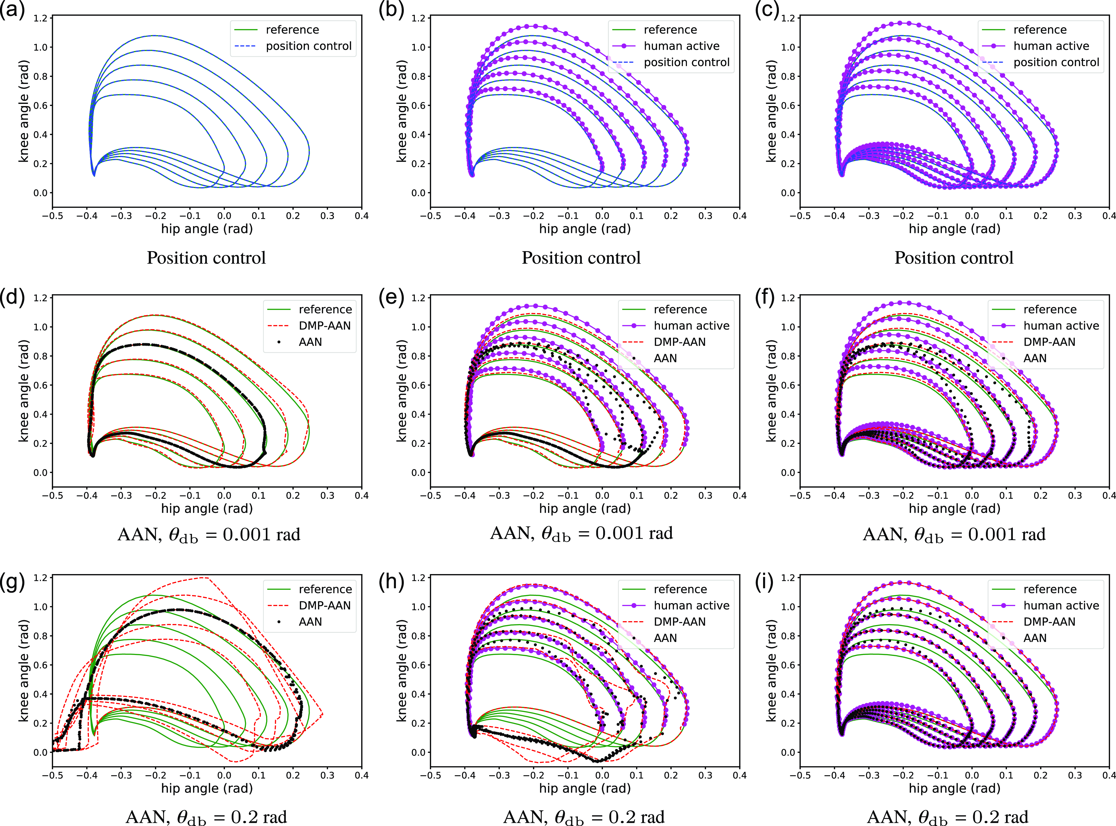
Figure 7. The comparison of joint angles for position control, conventional AAN control, and DMP-AAN control with varying gait patterns. The left, middle and right columns of sub-figures correspond to the passive state, partially active state and active state of the patient, respectively. The top, middle and bottom rows of sub-figures correspond to position control, conventional AAN control and DMP-AAN control of the exoskeleton robot. The green solid curves are reference joint angles reproduced by DMP, and the purple curves are joint angles from patient’s voluntary movement. The blue dashed curves, the black dot curves and the red dashed curves are actual joint angles for position control, conventional AAN control and DMP-AAN control of the exoskeleton robot, respectively.

The comparison of interaction forces is shown in Fig. 8, where interaction forces vary with different subject states and different exoskeleton control approaches. For position control, there is always an interaction force, because the exoskeleton leg often forces the subject’s leg to accurately track the reference joint angle. If the actual joint angle is different from the reference, the interaction force will be bigger (Fig. 8(a)) since there is a conflict between the subject’s leg and the exoskeleton leg. For AAN control, since the approach offers some space in the virtual tunnel for the subject to voluntarily move the leg, the interaction forces are smaller than position control and different with different $\theta _{\mathrm{db}}$ . For example, in sub-figures of the second column in Fig. 8, the last row (with $\theta _{\mathrm{db}} = 0.2$ rad) of interaction forces is smaller than the second row of sub-figures (with $\theta _{\mathrm{db}}=0.001$ rad). This means with a small $\theta _{\mathrm{db}}$ , the exoskeleton forces the subject’s joint to move along the reference joint angle, while a big $\theta _{\mathrm{db}}$ offers the subject more free space to move on his own. In the free space, there is only a guide torque to lead the joint to move along the reference joint angle instead of restricting the joint to accurately track it.

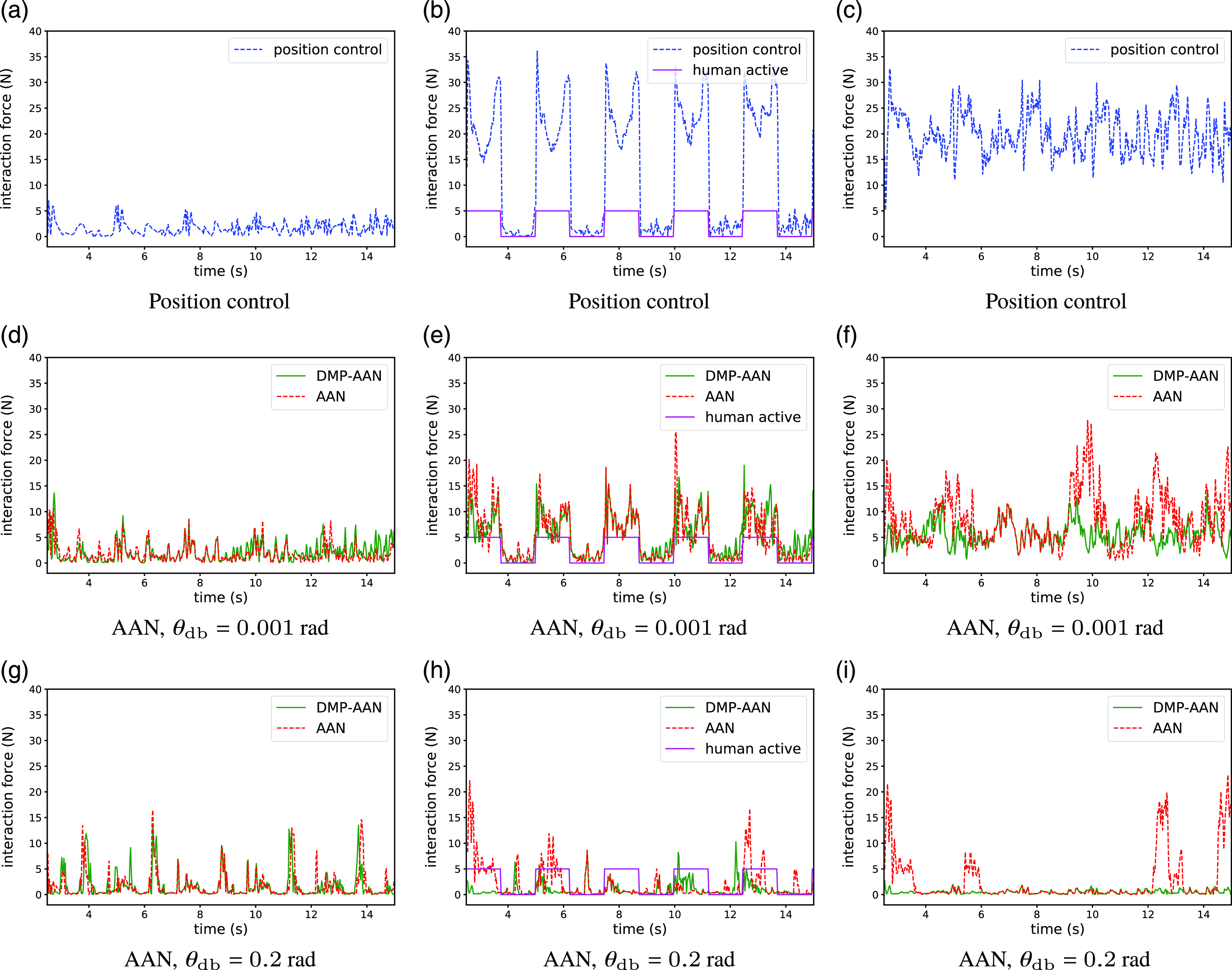
Figure 8. Comparison of interaction forces for position control (blue), conventional AAN control (red) and DMP-AAN control (green) with varying gaits. The presented curves are sum of interaction forces measured from force sensors. The left, middle and right columns correspond to the passive, partially active, and active states, respectively. These pictures separately correspond to the cases in Fig. 7. Note that in the middle column, the solid purple line represents the timing of the subject’s active movement, the positive value means the subject is actively moving, and zero means the subject is passively moving.

However, due to the fixed reference trajectory, conventional AAN control has less adaptability than DMP-AAN control with varying gait patterns. For example, in Fig. 7(a), with $\theta _{\mathrm{db}}=0.2$ rad, as the conventional AAN control offers the virtual tunnel around the fixed reference joint angle, the actual joint angle cannot adapt to the subject’s own movement. On the contrary, with DMP-AAN control, the subject can fully lead the exoskeleton to follow the subject’s voluntary movement to conduct an individualized gait pattern. The corresponding interaction forces are shown in Fig. 8(b), the interaction force for DMP-AAN is smaller than conventional AAN.

The comparison of mean interaction forces corresponding to Fig. 8 is shown in Table I. For the passive state, there is always a small interaction force for all control strategies because the paretic leg of the subject is moved by the exoskeleton active leg. Because of the absence of the subject’s active movement, to move the same leg with little muscle strength, the required mean interaction forces are similar. For the partially active state and the active state, the interaction force for AAN control is smaller than position control in most cases and varies with different $\theta _{\mathrm{db}}$ values. For the active state, we can find that with an appropriate $\theta _{\mathrm{db}}$ , there are much smaller interaction force for the AAN control compared to the position control. On the other hand, DMP-AAN has better performance on both joint angle tracking and smaller interaction forces than the conventional AAN while the subject is moving the leg actively on his own. As shown in the last item in Fig. 7(a) and Table I, with $\theta _{\mathrm{db}}=0.2$ rad, there is almost no interaction force, that means the subject can move the paretic leg fully on his own, which is very helpful for patient’s training with varying gait patterns. Above all, compared with the position control and conventional AAN control, the DMP-AAN control approach could improve the voluntary participation of the subject with varying gait patterns.

Table I. Mean interaction force (N).

4. Conclusions

This paper presents a novel approach for online gait learning and AAN control in post-stroke rehabilitation exoskeletons. The proposed approach encompasses the acquisition of joint angles from the healthy leg of the patient, generation of corresponding joint angles for the paretic leg, and the establishment of a virtual tunnel to facilitate voluntary movement of patients. The primary objective of this approach is to enhance gait training engagement specifically for patients exhibiting predominantly weakness. In comparison to conventional AAN control methods, the proposed approach demonstrates adaptability to diverse gait patterns, rendering it more suitable for individualized gait training regimens. To evaluate the efficacy of the proposed approach, experimental assessments were conducted on an exoskeleton robot employing healthy subjects. The experimental results indicate that the proposed DMP-AAN approach outperforms both position control and conventional AAN control techniques.